Scuola di Scienze
Dipartimento di Fisica e Astronomia Corso di Laurea Magistrale in Fisica
Graph-based analysis of brain structural
MRI data in Multiple System Atrophy
Relatore:
Dott.ssa Claudia Testa
Correlatore:
Prof.ssa Paola Fantazzini
Presentata da:
Riccardo Gubellini
Abstract
Il lavoro che ho sviluppato presso l’unità di RM funzionale del Policlinico S.Orsola-Malpighi, DIBINEM, è incentrato sull’analisi dei dati strutturali di risonanza magnetica mediante l’utilizzo della graph theory, con lo scopo di valutare even-tuali differenze tra un campione di pazienti affetti da Atrofia Multi Sistemica (MSA) e uno di controlli sani (HC).
L’MSA è una patologia neurodegenerativa sporadica e progressiva caratte-rizzata da disturbi del movimento e dalla disfunzione del sistema nervoso ve-getativo. Essa si divide in due sottotipi: MSA-P in cui predominano sintomi parkinsoniani ed MSA-C caratterizzata da deficit cerebellari. Circa un terzo delle persone affette da MSA sperimentano una particolare apnea respiratoria, chiamata Stridor. Questo sintomo può essere particolarmente pericoloso e por-tare anche alla morte. Nello studio sono stati confrontati tra loro tre coppie di gruppi: HC vs MSA, No-stridor vs Stridor, e MSA-C vs MSA-P.
I grafi sono strutture matematiche definite da nodi e links, che trovano ap-plicazioni in molte discipline diverse tra loro. In campo neurologico, a scopo di ricerca, la graph theory è stata recentemente applicata a dati di functional Magnetic Resonance Imaging (fMRI) e Diffusion Weighted Imaging (DWI) con lo scopo di comprendere il funzionamento del cervello visto come network. I network così costruiti fanno riferimento alla connettività strutturale (DWI) e funzionale (fMRI). Un altro tipo di approccio è quello di considerare un nuo-vo tipo di connettività, bastato su misure di correlazione anatomiche come la Cortical Thickness, oppure, come per questa tesi, su misure di correlazione volumetriche tra le diverse regioni del cervello.
Per poter costruire un grafo per ogni gruppo il primo step è stato ottenere la parcellizzazione delle immagini strutturali cerebrali, successivamente quello di valutare i volumi delle regioni cerebrali, e in seguito le correlazioni tra esse. Una volta costruiti i grafi è stato possibile calcolare i parametri topologici, globali e locali, che ne caratterizzano struttura ed organizzazione. Nei vari confronti fatti fra gruppi non sono state riscontrate differenze nelle proprietà globali del network. L’analisi regionale invece ha evidenziato un’ alterazione del gruppo dei pazienti affetti da MSA rispetto agli HC relativa a regioni che appartengono al network centrale autonomico, particolarmente colpito dalla malattia. Un’al-terazione analoga, riguardante specificatamente le misure di Node Betweenness e Node Degree, è stata trovata anche nel confronto fra i soggetti affetti e non affetti da stridor. Sono state inoltre riscontrate alterazioni nella organizzazione modulare dei gruppi presi in esame. E’ stata mostrata infatti una segregazione nel network motorio cortico-subcorticale nel gruppo di pazienti MSA rispetto agli HC (senza differenza fra i sottotipi C e P), in linea con la patologia.
Questa analisi ha mostrato la possibilità di indagare la funzionalità dei net-work cerebrali e della loro architettura modulare con misure strutturali quali la covarianza dei volumi delle varie regioni cerebrali in gruppi di soggetti.
Contents
1 Magnetic resonance 9
1.1 Theory of nuclear magnetic resonance . . . 9
1.2 Spin-echo sequence . . . 11
1.3 Relaxation times . . . 13
1.4 Spatial position: K-space encoding . . . 14
1.5 Gradient echo sequences . . . 15
1.5.1 Fast Spoiled Gradient Recalled Echo (FSGRE) . . . 17
2 Multiple System Atrophy 18 2.1 Historical background . . . 18
2.2 Epidemiology . . . 19
2.3 Clinical characteristics . . . 19
2.4 Motor involvement . . . 19
2.5 Sleep and breathing disorders (Stridor) . . . 20
2.6 Cognitive function . . . 20
2.7 Pathology and pathogenesis . . . 20
2.8 Neuroimaging . . . 21
2.9 Diagnostic criteria . . . 22
2.10 Neuroimaging criteria . . . 22
3 Graph theory 24 3.1 History of graph theory . . . 24
3.2 Definitions . . . 26
3.2.1 The nature of links . . . 26
3.2.2 Multiplicity of links . . . 27
3.2.3 Weighted/unweighted graph . . . 27
3.3 Applications . . . 28
3.3.1 Complex brain networks . . . 29
3.4 How to construct a brain graph . . . 30
3.4.1 Nodes and links decisions . . . 31
3.4.2 Correlations and adjacency matrices . . . 31
3.5 Measures . . . 31
3.5.1 Node degree and degree distribution . . . 32
3.5.2 Shortest path length . . . 32 3
3.5.3 Connected components . . . 32
3.5.4 Clustering coefficient . . . 33
3.5.5 Path length and Efficiency . . . 33
3.5.6 Hubs, centrality and robustness . . . 34
3.5.7 Modularity . . . 34
3.5.8 Random, scale-free and small-world networks . . . 35
4 Materials and methods 37 4.1 Participants . . . 37
4.2 MRI data acquisition . . . 38
4.3 Data pre-processing . . . 38
4.3.1 Brain Extraction Tool (BET) . . . 39
4.3.2 Lesion Filling (LF) . . . 41
4.3.3 Freesurfer . . . 41
4.3.4 Brainstem regions . . . 42
4.4 Construction of structural correlation network . . . 43
4.4.1 Node decision . . . 43
4.4.2 Volume of ROIs . . . 47
4.4.3 Definitions of correlations matrices . . . 47
4.4.4 Thresholding and Adjacency Matrices . . . 48
4.5 Data analysis . . . 49
4.5.1 Network analysis . . . 49
4.5.2 Statistical analysis . . . 50
4.5.2.1 Clinical data . . . 50
4.5.2.2 Comparison of correlations matrices between groups 50 4.5.2.3 Comparison of network measures between groups 51 4.6 Network visualization . . . 52
5 Results 53 5.1 Clinical variability . . . 53
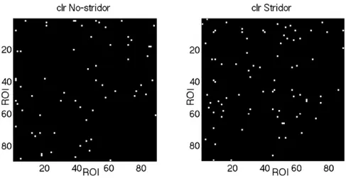
5.2 Comparison of correlations matrices between groups . . . 54
5.2.1 Correlation analysis . . . 54
5.2.2 False discovery rate matrices . . . 63
5.2.3 Z-Statistic . . . 67
5.3 Topological parameters and group analysis . . . 67
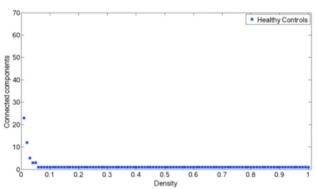
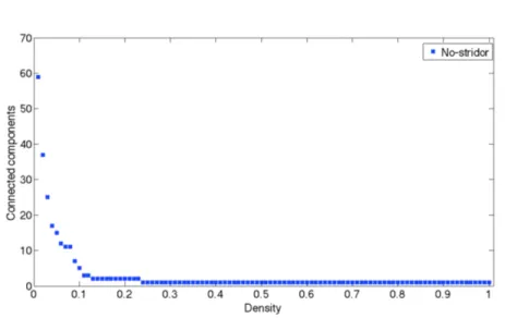
5.3.1 Connected components . . . 67
5.3.2 Comparison between groups across density . . . 71
5.3.2.1 Healthy controls vs MSA . . . 71
5.3.2.2 No-stridor vs Stridor . . . 80
5.3.2.3 MSA-C vs MSA-P . . . 89
5.3.3 Regional analysis . . . 98
5.3.3.1 Healthy controls vs MSA . . . 99
5.3.3.2 No-stridor vs Stridor . . . 101
5.3.3.3 MSA-C vs MSA-P . . . 102
5.3.4 AUC . . . 104
5.3.4.2 No-stridor vs Stridor . . . 106
5.3.4.3 MSA-C vs MSA-P . . . 108
5.3.5 Modularity . . . 110
5.3.5.1 Healthy controls vs MSA . . . 110
5.3.5.2 No-stridor vs Stridor . . . 112
5.3.5.3 MSA-C vs MSA-P . . . 114
5.3.5.4 Modularity visualization . . . 116
6 Discussion 118
Introduction
Multiple System Atrophy (MSA) is a neurodegenerative movement disorder characterized by a combination of the following signs and symptoms: autonomic dysfunction, parkinsonism (muscle rigidity, tremor and slow movement), ataxia (poor coordination and unsteady walking). The cause of MSA is unclear and no specific risk factors have been identified. It is divided in two sub-types: MSA-P with a prevalence of parkinsonian symptoms and MSA-C with predominant cerebellar ataxia. Brain MR images in patients with MSA may reveal atrophy in cerebellum and brainstem areas. Approximately one-third of the patients with MSA suffer of a breathing abnormality called Stridor, that is a risk factor for sudden death. In this study we decided to considered the following groups: 36 MSA patients and 27 healthy controls (HC) . The MSA group was divided into two sub-types: 20 MSA-C and MSA-P. The MSA group was also divided into two sub-groups: 22 patients without stridor and 14 patients with stridor. All these patients are followed by IRCCS “Istituto delle Scienze Neurologiche, DIBINEM, Bologna”.
A conventional screening to MSA patients includes a volumetric T1-weighted
(T1-w) sequence that allows to have an excellent spacial definition of brain.
Fur-thermore, T1-w sequences help the distinction between different brain regions.
For these reasons this sequence is used to segment Magnetic Resonance (MR) brain images.
Once brain images were segmented we evaluated volumes of different brain region. A key part of the thesis was the choice of the ROIs for the construction of the network targeted to the study of MSA patients. For this reason we have chosen to add seven ROIs belonging to the the infratentorial area, whose volumes are estimated with a semi-automatically procedure. To our knowledge, this kind of approach has been experienced for the first time by us. Although the procedure requires a manual drafting of infratentorial ROIs, it has been automated by registering on the 3D space of the individual subject.
The present work wants to investigate possible differences between groups us-ing a relatively new methodological approach to investigate neuroimagus-ing data, called graph-based analysis. The graph theory is the study of graphs, which are mathematical structures, made by nodes and edges that connect them. The graph theory is used to model many types of relations and processes and it can be applied in different fields of study. In the present work, we performed a graph theoretical analysis on structural MRI data to construct a network for
each group, with the aim of characterizing the morphometric covariance be-tween brain regions. Using MR structural T1-w imaging it is possible to obtain
images with high resolution and really good contrast used to perform a detailed segmentation and extract volumes of different brain regions (using automatic software like Freesurfer) in order to create anatomical covariate networks. This objective may be achieved measuring global and regional topological properties and the modular organization from the resulting network derived from anatom-ical covariance. This kind of graph-based analysis applied on MSA patients and healthy controls has never been done before.
This thesis is organized as follows: the first chapter describes the basic principles of MRI technique, with a detailed explanation of the gradient echo sequences. The second chapter introduces the MSA, talking about clinical char-acteristics, pathology and pathogenesis. The third chapter goes into the graph theory, starting from the description of what a graph is and how a graph can be generated, and ending with a description of several possible measures that can be performed on these networks. The fourth chapter reports the methods and the materials that we used during the entire analysis and the fifth one shows the obtained results. The sixth chapter provides the discussion and the inter-pretation of the results, while the seventh chapter analyzes the possible future directions which might be explored.
Magnetic resonance
Nuclear magnetic resonance (NMR) is a physical phenomenon in which nuclei in a magnetic field absorb and re-emit electromagnetic radiation. This energy is at a specific resonance frequency which depends on the strength of the magnetic field and on the magnetic properties of the isotope of the atoms.
Historically, NMR was first described and measured in molecular beams by Isidor Rabi in 1938, by extending the Stern–Gerlach experiment, and in 1944, Rabi was awarded the Nobel Prize in Physics for this work. In 1946, Felix Bloch and Edward Mills Purcell expanded the technique for use on liquids and solids, for which they shared the Nobel Prize in Physics in 1952. Another important contribution was given by Richard Robert Ernst that awarded the 1991 Nobel Prize in chemistry for the development of the method of high-resolution NMR spectroscopy. Paul Christian Lauterbur and Peter Mansfield awarded the 2003 Nobel Prize in Medicine for the production of the first 2D and then 3D MR images.
1.1 Theory of nuclear magnetic resonance
Isaac Rabi, thought the atom is a two level system with two possible configura-tions: ground state and excited state. He proved that if an electromagnetic field (frequency !) is applied to an atom with the same frequency !0= (Ee~Eg), it
could change its state from ground state energy Eg, to and excited state
en-ergy Ee, this phenomenon is known as resonance. In this model the system
is approximated with a two possible level configurations and without an ex-ternal electromagnetic filed the probability of transition from one state to the another one is approximately equal to zero. Nuclear Magnetic Resonance uses the fact that nuclei have a magnetization associated with them. All nucleons, that is neutrons and protons, composing any atomic nucleus, have the intrin-sic quantum property of spin that can be up or down. In human tissues the most common unpaired proton nucleus is hydrogen,1H, it is contained in
wa-ter molecules H20 , and in fat CH2 [1]. If1H is considered like a proton,
when a static magnetic field is applied, a splitting of nuclear state occurs. This interaction can form two energetic levels Eeand Egcalled Zeeman’s levels. The
energetic gap between the two levels is:
4E = ~B0 (1.1)
The proton spins form a magnetization vector M0 which has the same
di-rection of the external field, B0. Spins precess around B0 (Figure 1.1) with a
frequency called Larmor frequency:
!L= B0 (1.2)
where is the gyromagnetic ratio characteristic of the nuclei (1H : =
42.58M Hz T ).
Figure 1.1: Nuclear spin precession respect to a static magnetic field B0
When a radiofrequnecy (RF) is applied with a weak magnetic field, the spins will also precess around the new magnetic field B1. The net magnetization M0
has a spiral motion around the B0 axis, called “nutation”. We can have the
resonance condition of the hydrogen nuclei if the frequency of the RF pulse ! is the same of !L. This condition the RF pulse can give energy to the protons,
and we can have an excited state of the atom. Adjusting duration and intensity of the RF pulse, we can flip the net magnetization M0nutation angle. Rotation
to the desired angle can be obtained by:
✓ = B1⌧ (1.3)
where ⌧ is the duration and B1 represent the strength of the RF pulse.
Protons are first excited with the RF pulse, then the magnetization relaxes and returns exponentially aligned with the B0 axis. Relaxation is defined by two
time by which the magnetization aligns with the B0axis (z axis). T2is related
to the energy exchange between protons and describes the relaxation in the xy plane orthogonal to the z axis.
Relaxation of protons produces a FID (Free Indution Decady) signal that can be detected by a receiver coil (Figure 1.2). T1and T2can be used to characterize
different tissues, for example in liquid they are very similar (few seconds), in solid T1 is long (few minutes) and T2 is very short (few microseconds). T2 is
used to be smaller or equal to T1and in human tissue the value of T1is between
150 and 1000 milliseconds [2].
Figure 1.2: RF pulse excitation and FID relaxation.
1.2 Spin-echo sequence
Spin-Echo sequence (SE) in used to measure the relaxation signal. First of all protons are excited with a RF pulse (called 90°) that brings the initial magneti-zation in the xy plane. Spins are in speared in the xy plane, precessing around z axis with different angular velocities. Erwin Hahn in his 1950 paper, applied a 180° RF pulse to invert the precession of spins, and return them to the begin-ning position. The phenomenon may be better understood by breaking it down into the following steps (Figure 1.3):
Figure 1.3: A. The vertical red arrow is the average magnetic moment of a group of spins, such as protons. All are vertical in the vertical magnetic field and spinning on their long axis, but this illustration is in a rotating reference frame where the spins are stationary on average. B. A 90 degree pulse has been applied that flips the arrow into the horizontal (xy) plane. C. Due to local magnetic field inhomogeneities (variations in the magnetic field at different parts of the sample that are constant in time), as the net moment precesses, some spins slow down due to lower local field strength (and so begin to progressively trail behind) while some speed up due to higher field strength and start getting ahead of the others. This makes the signal decay. D. A 180 degree pulse is now applied so that the slower spins lead ahead of the main moment and the fast ones trail behind. E. Progressively, the fast moments catch up with the main moment and the slow moments drift back toward the main moment. F. Complete refocusing has occurred and at this time, an accurate T2echo can be
measured with all T⇤
2 effects removed.
The signal acquired for the Spin-Echo sequence is:
S = N (H)(e T E/T2⇤(1 eT R/T1)) (1.4)
where N(H) is the number of protons and M0↵N (H). Which was before
flipped in the xy plane by the 90 degree RF pulse, will return aligned to the z axis; this is called T1 recovery of the relaxation signal. T2⇤ concerns spin-spin
interaction and is influenced by magnetic field inhomogeneities: 1 T⇤ 2 = 1 T2 + 4B (1.5)
M0 relaxation curves can be plotted on the same graph as we can see in
Figure 1.4: Recovery and decay curves plotted on the same graph
1.3 Relaxation times
Tissues are composed by different molecules and have different frequencies by which they release energy [3]. It is possible to define a function J(!) that de-scribes the probability of a population to have a certain frequency for thermal motions. In Figure 1.5, we can see different curves for different materials. For example lipids as viscous liquids have the bigger probability of release the Lar-mor frequency !0acquired during the excitation so they relax faster in the T1
dependent sequence.
Figure 1.5: Spectrum of tumbling motions for different materials. Since each material has characteristic relaxation times, we can acquire im-ages from the same tissue with different information, for example T1 or T2
weighted images. As we can see in Figure 1.6 White Matter (WM) has a shorter T1 than Gray Matter (GM) so we can use T1-dependent images to show
gray-white matter contrast. While gray-white matter acts in a similar way to fat because it is composed by protons of phospholipids, Cerebro Spinal Fluid (CSF) acts like water and it has the longest relaxation times.
Figure 1.6: In the left panel: T1 and T2 decay curves of fat, water and solid
tissue. In the right panel: T1 and T2 decay curves of CSF, white matter and
grey matter.
1.4 Spatial position: K-space encoding
It is important to associate a spatial position to the acquired signal; we can do that using magnetic field gradients. Phase and frequency encoding are used to associate the acquired signal with a spatial position. Images are first acquired as a spectrum, that could be represented in a k-space, than the frequency-phase space is transformed back to the spatial coordinates by Fourier transform. As shown in Figure 1.7 a gradient is first applied due to excite a specific slice in a specific direction z (G slice), then two gradients orthogonal to the direction of the slice are applied in directions x and y. The first one characterized the frequency encoding (G freq) and the other the phase encoding (G phase). The gradient to select the slice is applied at the same time of the 90° pulse, while the frequency gradient is applied during the readout of the echo, when all the frequencies are acquired in a selected phase [4].
Figure 1.7: Pulse gradient sequence for a 3D spatial sampling.
1.5 Gradient echo sequences
Gradient echo sequences (GRE) are alternative techniques to spin echo se-quences, differing from them in two principal points:
• utilization of gradient fields to generate transverse magnetization • flip angles of less than 90°
Compared to the spin echo and inversion recovery sequences, GRE sequences are more versatile. It is not only the basic sequence varied by adding dephasing or reshaping gradient at the end of the sequence, but there is a significant extra variable to specify in addition to the usual TR and TE. This in the flip or tip angle of the spins.
In gradient-echo (GE) or gradient recalled echo (GRE), it is used an RF pulse to flip M0with an angle ↵ < 900[5]. It is not applied the 180° pulse but it
is used a gradient to refocus the spins, thus the magnetic field inhomogeneities are even present and there is a weighting on T⇤
2 instead of T2.
The GE sequences have a low weighting on T1, because Mz does not have
time to relax. However to increase the T1-weighting is uses the spoiled GRASS
(gradient recalled acquisition in the steady state) or SPGR (spoiled GRASS): this sequence “spoils” the steady-state transverse magnetization [6]. The world “spoiling” refers to the elimination or spoiling of the stady-state transverse mag-netization. This task can be accomplished in different ways:
• by applying RF spoiling
• by lengthening TR
In the Figure 1.8 is represented the spoiled GRE sequence by using gradient spoilers.
Figure 1.8: Spoiled GRE using gradient spoilers
Because the spoiled-GRE technique is specifically designed to disrupt trans-verse (T2) coherences, its major benefit and use is in producing T1-weighted
images. Nevertheless, both spin density- and T⇤
2-weighting can be achieved by
appropriate selection of parameters. As a result of this versatility and the abil-ity to acquire images in either 2D or 3D modes, spoiled-GRE sequences are now ubiquitously used for MR imaging of virtually every body part.
The signal from a spoiled-GRE sequence depends on three operator-selectable parameters (TR, TE, and flip angle a) plus three intrinsic tissue parameters (T1, T2⇤, and spin-density [H]). Assuming a longitudinal steady-state has been
reached and perfect spoiling, the signal (S) of a spoiled GRE sequence is given by [7]:
S = k[H] sin↵(1 e
T R/T1)
(1 (cos↵)e T R/T1)e
T E/T2⇤ (1.6)
where k is a scaling factor. Setting dS/d↵ = 0 we find that the signal is maximized when ↵ = ↵E, the Ernest angle where ↵E = arccos(e T R/T1).
Although the Ernest angle gives the highest signal for a given tissue for a certain T R/T1combination, it does not necessarily maximize image contrast between
two different tissues.
Discussing the equation 1.6 is important to consider some important thinks: • Signal is always proportional to spin density [H], an effect that never be
removed. • TE controls T⇤
2-weighting. The only place T2⇤appears in the equation is
in the term e T E/T⇤
2. When TE is large, this terms dominates. When TE
is small, this term approaches unity and the T⇤
• Flip angle controls T1-weighting. A small flip angle minimizes T1-weighting
because the longitudinal magnetization of various tissues are not different much by such a small angular displacement.
• TR controls T1-weighting. Note that all occurrences of TR in the
equa-tion are in terms of the form e( T R/T1). When TR is small, this term
becomes large and T1-weighting increases. Conversely, when TR is long,
T1-weighting is minimized.
1.5.1 Fast Spoiled Gradient Recalled Echo (FSGRE)
It is true that GRE techniques are generally faster than SE techniques, although the Fast Spin Echo (FSE) technique may be equally fast. However, there are additional methods that can further increase the speed of scanning like the FSGRE technique. In order to make the GRE technique is necessary to employ ultra shorts TRs and TEs to reduce the sequence time. This is achieved by the use of the following:
1. Fractional echo 2. Fractional RF
3. Reduction in the sampling time Ts (by increasing the bandwidth (BW), which is the frequency range between lowest and highest attainable fre-quency)
Basically, by using a fraction of the echo and a fraction of the pulse, we can in effect decrease TE. Increasing the BW results in a reduction of the sampling time. The trade-off here is a reduction of SNR because it is proportional to
1 p
BW. The sequence time is now given by: SeqT ime = T E + T s/2 + T0where
Multiple System Atrophy
Multiple system atrophy (MSA) is a neurodegenerative movement disorder char-acterized by parkinsonism associated with various combinations of autonomic, pyramidal and cerebellar signs.
2.1 Historical background
In 1900, Dejerine and Thomas provided the first report of sporadic olivopon-tocerebellar atrophy (OPCA), a disease that later would have become a part of the spectrum of MSA [9]. Orthostatic hypotension as a manifestation of au-tonomic failure was described in 1925 [10]. In 1960, Shy and Drager reported patients with autonomic features of orthostatic syncope, impotence, and bladder dysfunction who went on to develop gait abnormalities, tremor, and fascicula-tions among other symptoms and signs. This disorder became known as the ShyDrager syndrome [11].
Also in 1960, the first cases of a predominantly asymmetric parkinsonian syndrome manifested primarily by akinesia and rigidity were reported. The authors suggested that striatonigral degeneration was the pathologic correlate for these cases.
In 1969, the term "multiple system atrophy" was introduced to encompass all three clinical syndromes: olivopontocerebellar atrophy, ShyDrager syndrome, and striatonigral degeneration. Striatonigral degeneration was later redefined as MSA with predominant parkinsonism (MSA-P), while olivopontocerebellar atrophy was redefined as MSA with predominant cerebellar ataxia (MSA-C) [12]. When autonomic failure predominates, the term ShyDrager syndrome may be used.
The discovery that glial cytoplasmic inclusions with alpha synuclein as a major component are the pathologic hallmark of the three clinical syndromes confirmed the suspicion that they were actually different manifestations of the same disease. Beginning in the 1990s, consensus groups developed guidelines to define MSA [13].
2.2 Epidemiology
The estimated prevalence of MSA is between 2 to 5 cases per 100.000 population [14]. In a metaanalysis of 433 pathologically proven cases of MSA, the mean age of onset was 54 years (range 31 to 78) (younger than Parkinson disease). Similarly, European registry studies have reported onset at a mean age of 56 to 60 years [15]. In these registries, MSA affects men and women about equally. However, other studies have reported that men are affected two to nine times more often than women. This finding may be secondary to earlier recognition of impotence as a major diagnostic feature in men. There is no specific racial predilection, and the disease has been reported in Caucasian, African, and Asian populations.
Although MSA is considered a sporadic disease, there are several reports of rare patients with probable or possible familial MSA [16].
2.3 Clinical characteristics
The main clinical features of MSA are akineticrigid parkinsonism, autonomic failure including urogenital dysfunction, cerebellar ataxia, and pyramidal signs in varying combinations. The onset of disease is marked by the initial clinical manifestation of any of its characteristic motor or autonomic features. However, the neuropathologic changes probably begin several years before the disease becomes symptomatic [17].
2.4 Motor involvement
The motor presentations of MSA are classified into two separate but overlapping clinical subtypes:
• MSA with predominant parkinsonism (MSA-P) subtype • MSA with predominant cerebellar ataxia (MSA-C) subtype
In most studies from Europe and North America, cases of MSA-P outnumber MSA-C by between two and four to one. This contrasts with studies from Japan, which report MSA-C as more common than MSA-P. The predominant motor feature can change over time with disease progression. Thus, the designation of MSA-P or MSA-C refers to the predominant motor problem at the time the patient is evaluated. As an example, in a European study of 437 patients from 19 centers, the proportion of patients classified as MSA-P and MSA-C was 68 and 32 percent, respectively. However, among the entire cohort, parkinsonism and cerebellar ataxia were present in 87 and 64 percent, respectively [18].
Parkinsonism in MSA-P is characterized by akinesia/bradykinesia, rigidity, postural instability, and an irregular jerky postural and action tremor. Up to two-thirds of patients with MSA have this tremor involving the arms. Although much less common than in idiopathic Parkinson disease, rest tremor occurs in
as many as one-third of patients with MSA-P. Other warning signs that herald parkinsonism in MSA include postural instability and falls (usually within three years of motor onset), pyramidal signs, including extensor plantar responses, and rapid progression regardless of dopaminergic treatment [19]. Additional move-ment disorders associated with MSA-P may include stimulus-sensitive cortical myoclonus, hemiballism and chorea, and dystonia unrelated to dopaminergic therapy.
In contrast to MSA-P, the motor features of MSA-C involve predominant cerebellar dysfunction that manifests as gait ataxia, limb ataxia, ataxic dysarthria, and cerebellar disturbances of eye movements [20].
2.5 Sleep and breathing disorders (Stridor)
Sleep and breathing abnormalities are common in MSA. At least two-thirds of patients have rapid eye movement (REM) sleep behavior disorder. The content of the dreams can be vivid, violent, and frightening. The usual muscle atony in REM sleep is lost, and patients may act out their dreams. For example, patients may talk or shout during sleep and may strike out at their bed partner. This feature of MSA often precedes the motor manifestations, sometimes by decades. It tends to improve as the disease progresses .
Nocturnal or diurnal laryngeal stridor occurs in approximately one-third of patients with MSA [21]. It is a risk factor for sudden death in MSA. The sound of stridor is high pitched and occurs with inspiration. Patients may also experience sleep apnea and involuntary sighs or gasps during the day. Snoring may increase from premorbid level or may be new onset. These abnormalities of breathing are uncommon in idiopathic Parkinson disease and in other atypical parkinsonian syndromes. However, REM sleep behavior disorder and obstructive sleep apnea are not specific to MSA. REM sleep behavior disorder is frequently present in idiopathic Parkinson disease and some forms of spinocerebellar ataxia [22].
2.6 Cognitive function
Cognitive function in MSA tends to be relatively well preserved compared with idiopathic Parkinson disease and other atypical parkinsonian syndromes, possi-bly reflecting a lesser degree of cortical involvement in MSA and the younger age of onset. Nevertheless, although cognitive impairment in MSA is uncommon, it does occur and its presence does not exclude MSA as a clinical diagnosis in patients who have classic symptoms and signs of the disorder [23].
2.7 Pathology and pathogenesis
The cause of MSA is unknown. One postulated mechanism involves prion-like spreading of aberrant alphasynuclein from neurons to glia through functionally
connected networks, thereby leading to glial and myelin dysfunction and an inflammatory cascade that promotes secondary neurodegeneration.
Neuronal inclusions of various types also are present in the majority of pa-tients with MSA. Myelin degeneration is characteristic of MSA. A small casec-ontrol study found a significantly greater degree of white matter hyperintensities on MRI scans from patients with MSA compared with scans from patients with Parkinson disease and healthy controls. This finding could be related to the loss of myelin or to cerebral hypoperfusion from orthostatic blood pressure fluctua-tions in MSA [24].
In idiopathic Parkinson disease, positron emission tomography imaging stud-ies have indicated that dysautonomia is caused by peripheral nervous system dysfunction, particularly myocardial sympathetic denervation. In contrast, the peripheral autonomic system appears to be spared in MSA. Some persistence of autonomic tone may be responsible for the frequently observed supine hyper-tension in MSA.
Motor abnormalities seen in MSA-P are due primarily to neuronal loss and gliosis in the substantia nigra, putamen, caudate, and globus pallidus . One of the features that distinguish MSA and other atypical parkinsonian syndromes from idiopathic Parkinson disease is the lack of dramatic and sustained response to levodopa. The extent of putaminal involvement may determine the poor response to levodopa.
In contrast to MSA-P, the cerebellar ataxia and pyramidal signs that char-acterize the MSA-C subtype are secondary to degeneration of the cerebellar Purkinje cells, middle cerebellar peduncles, inferior olivary nuclei, basis pontis, and pontine nuclei. However, a majority of patients with MSA-P probably have subclinical loss of nigral neurons based upon findings from SPECT imaging . Loss of cholinergic mesopontine neurons, combined with loss of locus ceruleus neurons and preservation of rostral raphe neurons, may contribute to REM sleep abnormalities often seen in MSA. Respiratory abnormalities may reflect loss of cholinergic neurons in the arcuate nucleus of the ventral medulla. Respiratory stridor, abnormal nocturnal ventilation, and pseudobulbar features are possibly secondary to brainstem pathology, and may involve the nucleus ambiguus [25].
2.8 Neuroimaging
Brain MRI in patients with MSA-P and MSA-C may reveal atrophy of the putamen, pons, and middle cerebellar peduncles [25]. On T2 MRI sequences,
signal changes include hypointensity of the posterior putamen, a hyperintense lateral putaminal rim, and hyperintensities of the middle cerebellar peduncles. These changes are supportive of the diagnosis of MSA rather than idiopathic Parkinson disease. However, they are not present in all patients with MSA. Furthermore, they are not specific for differentiating MSA from other atypical parkinsonian syndromes.
The "hot cross bun sign" refers to hyperintense T2signal in the shape of a
fibers. However, this is also a nonspecific finding that has also been described in patients with other causes of parkinsonism [26].
Diffusion weighted MRI in patients with MSA shows increased diffusivity (high apparent diffusion coefficient values) in the putamen, a finding that is sometimes observed in progressive supranuclear palsy. Preliminary data suggest that this technique can be used to monitor disease progression in MSA.
Positron emission tomography using (18F) fluorodeoxyglucose in patients
with MSA may reveal regional glucose hypometabolism in the striatum, brain-stem, and cerebellum, but the true sensitivity and specificity of these findings for differentiating MSA from Parkinson disease is uncertain.
2.9 Diagnostic criteria
The diagnosis of MSA is based upon the clinical features. No laboratory or imaging studies are diagnostic, particularly since findings are often normal or equivocal in early disease. Neuroimaging can be helpful in excluding other con-ditions and may show signs such as putaminal atrophy, slitlike signal change at the posterolateral putaminal margin, and hypointensity of the putamen relative to the globus pallidus [27].
A diagnosis of definite MSA is based upon postmortem pathology show-ing alpha-synuclein-positive glial cytoplasmic inclusions with neurodegenerative changes in striatonigral or olivopontocerebellar structures [28]. The clinical di-agnosis of probable MSA during life requires the following features:
• A sporadic, progressive, adult onset (>30 years old) disease.
• Autonomic failure involving either urinary incontinence (inability to con-trol the release of urine from the bladder, with erectile dysfunction in males) or an orthostatic blood pressure decrease within three minutes of standing by 30 mmHg systolic or 15 mmHg diastolic.
• Either poorly levodoparesponsive parkinsonism (bradykinesia with rigid-ity, tremor, or postural instability) or a cerebellar syndrome (gait ataxia with cerebellar dysarthria, limb ataxia, or cerebellar oculomotor dysfunc-tion).
2.10 Neuroimaging criteria
Neuroimaging correlates of MSA lack sufficient sensitivity and specificity to be used as reliable markers of probable MSA. Nevertheless, current diagnostic criteria regard atrophy of putamen, middle cerebellar peduncle, or pons on MRI as supportive features for possible MSA-C or MSA-P [25].
Additional supportive features for MSA subtypes are as follows:
• In a patient with parkinsonian features but no cerebellar ataxia, hy-pometabolism of putamen, brainstem, or cerebellum on18F emission
to-mography (FDG-PET) is considered to be a supportive feature for possible MSA-P.
• In a patient with cerebellar ataxia lacking parkinsonian features, two addi-tional imaging features are considered to be supportive for possible MSA-C:
– Hypometabolism of the putamen on FDG-PET
– Presynaptic dopaminergic denervation in the striatum on functional imaging with single photon emission computed tomography (SPECT) or PET
Graph theory
Graph theory is branch of mathematics that deals with the formal description and analysis of graphs. A graph is defined simply as a set of nodes (vertices) linked by connections (edges), and may be directed or undirected. When de-scribing a real-world system, a graph provides an abstract representation of the system’s elements and their interactions.
3.1 History of graph theory
The origins of graph theory can be traced to Leonhard Euler who devised in 1736 a problem that came to be known as the "Seven Bridges of Konigsberg" (Figure 3.1). The problem originated in the city of Konigsberg [30], formerly in Germany but, now known as Kaliningrad and part of Russia, located on the river Preger. The city had seven bridges, which connected two islands with the main-land via seven bridges.
Figure 3.1: The seven bridges of Konisberg
People staying there always wondered whether was there any way to walk 24
over all the bridges once and only once. Euler came out with the solution in terms of graph theory. He proved that it was not possible to walk through the seven bridges exactly one time. He abstracted the case of Konigsberg by eliminating all unnecessary features. He drew a picture (Figure 3.2) consisting of “dots” that represented the landmasses and the line-segments representing the bridges that connected those land masses.
Figure 3.2: Konigsberg bridges problem
This simplifies the problem to great extent. Now, the problem can be merely seen as the way of tracing the graph with a pencil without actually lifting it. One can try it in all possible ways, but you will soon figure out, it is not possible. But Euler not only proved that its not possible, but also explained why it is not and what should be the characteristic of the graphs, so that its edge could be traversed exactly once. He came out with the new concept of degree of nodes. The “Degree of Node” can be defined as the number of edges touching a given node. Euler proposed that any given graph can be traversed with each edge traversed exactly once if and only if it had, zero or exactly two nodes with odd degrees. The graph following this condition is called Eulerian circuit or path. We can easily infer this theorem. Exactly two nodes are beginning and end of your trip. If it has even nodes than we can easily come and leave the node without repeating the edge twice or more.
In case of seven bridges of Königsberg, once the situation was presented in terms of graph, the case was simplified as the graph had just 4 nodes, with each node having odd degree. So, Euler concluded that these bridges cannot be traversed exactly once.
Using this theorem, we can create and solve number of problems. Suppose now, we want to make the graph created from bridges of Konigsberg, a Euler’s circuit. Now, as per Euler’s theorem we need to introduce a path to make the degree of two nodes even. And other two nodes can be of odd degree out of which one has to be the beginning and the other the endpoint. Suppose we want to start our journey from blue node and end at the yellow node. So, the two nodes can have odd edges. But somehow we need to edit the actual graph by adding another edge to the graph such that the two other nodes have even degree. So, the resulting figure is shown below (Figure 3.3).
Figure 3.3: Example of final Konigsberg bridges problem
3.2 Definitions
A graph is an ordered pair G = (V, E) comprising a set V of vertices or nodes together with a set E of edges.
3.2.1 The nature of links
An undirected graph (Figure 3.4) is a graph in which edges have no orientation. The edge (x, y) is identical to the edge (y, x). The maximum number of edges in an undirected graph without a loop is n(n 1)
2 .
Figure 3.4: Undirected graph
A directed graph (Figure 3.5) is a graph in which edges have orientations. It is written as an ordered pair G = (V, A). An arrow (x, y) is considered to be directed from x to y; y is called the head and x is called the tail of the arrow; y is said to be a direct successor of x and x is said to be a direct predecessor of y. If a path leads from x to y, then y is said to be a successor of x and reachable from x, and x is said to be a predecessor of y. The arrow (y, x) is called the inverted arrow of (x, y). A directed graph G is called symmetric if, for every arrow in G, the corresponding inverted arrow also belongs to G. A symmetric loopless directed graph G = (V, A) is equivalent to a simple undirected graph G0 = (V, E), where the pairs of inverse arrows in A correspond one-to-one with the edges in E.
Figure 3.5: Directed graph In this work we decided to use undirected graph.
3.2.2 Multiplicity of links
A simple graph, as opposed to a multigraph, is an undirected graph in which both multiple edges and loops are disallowed. In a simple graph the edges form a set (rather than a multiset) and each edge is an unordered pair of distinct vertices.
A multigraph is a graph which is permitted to have multiple edges. Thus two vertices may be connected by more than one edge. There are two distinct notions of multiple edges:
• Edges without own identity: The identity of an edge is defined solely by the two nodes it connects. In this case, the term "multiple edges" means that the same edge can occur several times between these two nodes. • Edges with own identity: Edges are primitive entities just like nodes.
When multiple edges connect two nodes, these are different edges. A multigraph (Figure3.6) is different from a hypergraph, which is a graph in which an edge can connect any number of nodes, not just two.
Figure 3.6: Examples of simple, non simple and non simple with loops graphs In this study we used multigraph without loops.
3.2.3 Weighted/unweighted graph
A weighted graph (Figure 3.7) is a graph in which a number (the weight) is assigned to each edge. Such weights might represent for example costs, lengths
or capacities, depending on the problem at hand. Some authors call such a graph a network. Weighted correlation networks can be defined by soft-thresholding the pairwise correlations among variables (e.g. gene measurements).
Figure 3.7: Weighted graph
In an unweighted graphs edges have no weight, so they simply show connec-tions between nodes.
For our study we decided to used unweighted graphs.
3.3 Applications
Everything in our world is linked: cities are linked by street, rail and flight networks. Pages on the internet are linked by hyperlinks. The different com-ponents of an electric circuit or computer chip are connected and the paths of disease outbreaks form a network. Scientists, engineers and many others want to analyze, understand and optimise these networks. And this can be done using graph theory.
Graph theory can be used to analyze whatever is linked. Everything in our world is linked: cities are linked by street, rail and flight networks 3.8. Pages on the internet are linked by hyperlinks. The different components of an electric circuit or computer chip are connected and the paths of disease outbreaks form a network. Neurons in our brain are linked by synapses.
For example, graph theory can be applied to road networks, trying to find a way to reduce traffic congestion. An other useful application is in flight net-works. Airlines want to connect cities in the most efficient way, moving the most passengers with the fewest possible trips. One area where speed and the best connections are of crucial importance is the design of computer chips. Integrated circuits (ICs) consist of millions of transistors which need to be connected. In recent years, there has been another important use of graph theory: the inter-net. Every page in the internet could be a vertex in a graph, and whenever there is a link between two pages, there is an edge between the corresponding vertices.
Figure 3.8: Example of flight networks
3.3.1 Complex brain networks
One of the most important applications of graph theory is the study of brain network. The are two main different approaches, one based on structural correla-tion and anotherone based on funccorrela-tion systems. Both structural and funccorrela-tional brain networks can be explored using graph theory through the following four steps (Figure 3.9):
1. Define the network nodes.
2. Estimate a continuous measure of association between nodes. This could be for example connection probability between two regions of an individ-ual diffusion tensor imaging data set, or the inter-regional correlations in cortical thickness or volume MRI measurements estimated in groups of subjects.
3. Generate an association matrix by compiling all pairwise associations be-tween nodes and usually apply a threshold to each element of this matrix to produce a binary adjacency matrix or undirected graph.
4. Calculate the network parameters of interest in this graphical model of a brain network and compare them to the equivalent parameters of a population of random networks.
Many studies focus upon functional connectivity, using correlation analysis to identify regional connections, either with EEG/MEG or fMRI [34]. There has been a similar boom in studies of structural connectivity. Many groups employ diffusion-weighted imaging and tractography to examine structural connectivity as a white matter phenomenon [35]. In contrast to DWI approaches, there has been a growing interest in brain structure networks based on morphometric measures of GM volume, cortical thickness, and surface area. Graph generated from these different kind of approach have been found to follow a smallworld network organization as suggested by the brain networks of other connectivity modalities [36].
3.4 How to construct a brain graph
A brain graph is a model of a nervous system as a number of nodes intercon-nected by a set of edges. First of all it is necessary to decide which spatial level is considered: microscale, mesoscale or macroscale
• Constructing human brain connectome at microscale levels means that every node corresponds to a neuron and every edge to a synapse. This case is not realistic because of the excessive number, variability and dynamics of these elements. The number of neurons is estimated to be around 1011
with about 1015 connections between them. Recording and tracing this
number of connections is not possible.
• The description of connection pattern at mesoscale level involves struc-tures that generally contain about 100 neurons each and they may repre-sent functional elements that are crucial for cortical information process-ing.
• The macroscale level is the most feasible organizational level for describing an accurate model of human connectome, with the definition of anatom-ically distinct brain regions and inter-regional connections. Most current
studies focus on macroscale networks, also because of technical limitations and computational demand.
After the choice of the description level, nodes and edges must be defined: the first ones generally correspond to Regions Of Interest (ROIs) derived from anatomical atlas or appropriate segmentation process, and the edges can be defined as functional or structural association between these ROIs.
3.4.1 Nodes and links decisions
According to Bullmore and Basset [32], a node should be a portion of the system that could be separable from the rest of the system. Generally, nodes represent brain regions, which are labelled by a particular atlas. The choice of a template is a very important and delicate step because it determines different network structures and different topological characteristics.
There is not a unified method to choose edge between nodes. They are differ-entiated on the basis of the type of the connectivity, which could be functional or structural, but also on the fact that they could have weights and directionality. We focused our attention on structural association between nodes, because we were interested in obtain the structural connectivity between brain regions, and not the functional one. More precisely we considered the correlations be-tween the volume of different brain regions.
3.4.2 Correlations and adjacency matrices
Due to create an unweighted graph is necessary to generate an adjacent matrix. In order to create this matrix we have to define the correlation matrix and than apply a threshold to all values of it: if aij ⌧ the corresponding element of the
adjacency matrix is set to 1; 0 otherwise.
There are two possible choice for the implementation process to the adjacent matrix:
• to choose an optimal value of threshold to be applied to the correlation matrix and to describe the topological parameters of the network only at that threshold;
• to choose different values of threshold and describe the network properties as a function of threshold (or connection density);
The adjacency matrix so defined corresponds to the final network.
3.5 Measures
Once the brain network is constructed it is possible to characterize it using different topological measures. Here we propose only a few of these measures.
In order to understand the graph measures below it is important to define some variable. N is the set of all nodes in the network, and n is the number of
nodes. L is the set of all links in the network, and l is number of links. With the expression (i, j) we refer to a link between nodes i and j, (i, j 2 N). In the equations that we can find in this chapter, aijis the connection status between
i and j: aij = 1 when link (i, j) exists (when i and j are neighbors); aij = 0
otherwise (aii= 0 for all i). We compute the number of links as l =Pij2Naij
(to avoid ambiguity with directed links we count each undirected link twice, as aij and as aji) [31].
3.5.1 Node degree and degree distribution
The degree of a node (Eq.3.1) is the number of connections that link it to the rest of the network.
ki=
X
j2N
aij (3.1)
This one of the most fundamental network measure and most other measures are linked to node degree. In random networks all connections are equally prob-able, resulting in a Gaussian and symmetrically centered degree distribution. Complex networks generally have non-Gaussian degree distributions, often with a long tail towards high degrees. The degree distributions of scale-free networks follow a power law [31].
3.5.2 Shortest path length
Shortest path length (Eq.3.2) is a basis for measuring the integration of the network. It represents the distance between nodes i and j .
dij=
X
auv2gi !j
auv (3.2)
Where g !is the shortest path (geodesic) between i and j.
3.5.3 Connected components
Connected component (or just component) of an undirected graph is a subgraph in which any two vertices are connected to each other by paths, and which is connected to no additional vertices in the super graph. For example, the graph shown in Figure 3.10 has three connected components. A vertex with no incident edges is itself a connected component. A graph that is itself connected has exactly one connected component, consisting of the whole graph.
Figure 3.10: A graph with three connected components
This measure is useful to understand when a graph is fully connected because the connected component is equal to 1.
3.5.4 Clustering coefficient
If the nearest neighbors of a node are also directly connected to each other they form a cluster. The clustering coefficient (Eq.3.3) quantifies the number of connections that exist between the nearest neighbors of a node as a proportion of the maximum number of possible connections. Random networks have low average clustering whereas complex networks have high clustering (associated with high local efficiency of information transfer and robustness). Interactions between neighboring nodes can also be quantified by counting the occurrence of small motifs of interconnected nodes. The distribution of different motif classes in a network provides information about the types of local interactions that the network can support.
C = 1 n X i2N P 2ti ki(ki 1) (3.3)
3.5.5 Path length and Efficiency
Path Length (Eq.3.4) is the minimum number of edges that must be traversed to go from one node to another. Random and complex networks have short mean path lengths (high global efficiency of parallel information transfer) whereas regular lattices have long mean path lengths. Efficiency is inversely related to path length but it is numerically easier to use to estimate topological distances between elements of disconnected graphs. The average over all pair wise efficien-cies is the Global Efficiency of the graph (Eq.3.5); the Local Efficiency (Eq.3.6) is the mean of the efficiencies of all subgraphs Gi of neighbors of each of the
vertices of the graph.
L = 1 n X i2N P j2N.j idij n 1 (3.4)
Eglob= 1 N (N 1) X i,j2N 1 di,j (3.5) Eloc= 1 N X i2N E(Gi) (3.6)
3.5.6 Hubs, centrality and robustness
Hubs are nodes with high degree, or high centrality. The centrality of a node measures how many of the shortest paths between all other node pairs in the network pass through it. A node with high centrality is crucial to efficient communication. The importance of an individual node to network efficiency can be assessed by deleting it and estimating the efficiency of the ‘lesioned’ network. Robustness refers either to the structural integrity of the network following deletion of nodes or edges or to the effects of perturbations on local or global network states.
3.5.7 Modularity
A graph can generally be subdivided or partitioned into subsets or modules of nodes (Figure 3.11). Modularity quantifies the extent to which the network can be decomposed into sub-networks that are more connected within modules than between modules. Several alternative algorithms have been proposed to find the mathematically optimal modular decomposition for a network. In general, the aim is to find the partition that maximizes the ratio of intramodular to inter-modular edges. Thus the nodes in any module will be more densely connected to each other than to nodes in other modules [?].
Popular methods for discovering the modules of a network consists in op-timizing modularity, that is to find the partition having the largest value of Q. Q = 1 2m X C2P X i,j2C [Aij kikj 2m] (3.7)
where A is the adjacent matrix of the network; m is the total number of edges and ki=PjAij is the degree of the node i. The indices i and j run over
Figure 3.11: Modularity
3.5.8 Random, scale-free and small-world networks
In random graphs each pair of nodes has an equal probability, p, of being con-nected. Large random graphs have Gaussian degree distributions. It is now known that most graphs describing real-world networks significantly deviate from the simple random-graph model (Figure 3.12) [39].
Figure 3.12: Small world
Some networks have degree distributions in the form of a power law: that is, the probability that a node has degree k is given as Prob (k) ~ k . In biological systems, the degree exponent l often ranges between 2 and 3, and the very gradual (‘heavy-tail’) power law decay of the degree distribution implies that the network lacks a characteristic scale: such networks are called ‘scale-free’ networks. Barabási and Albert demonstrated that scale-free networks can originate from a process by which each node that is added to the network as it grows, connects preferentially to other nodes that already have high degree [40]. Scale-free networks are unlikely if the attachment of connections is subjected to physical constraints or associated with a cost. Therefore, physically embedded networks, in which nodes have limited capacity for making connections, often do not have pure power law degree distributions but may instead demonstrate exponentially truncated power law degree distributions, which are associated with a lower probability of very high degree nodes.
Originally described in social networks, the ‘small-world’ property combines high levels of local clustering among nodes of a network and short paths that globally link all nodes of the network. This means that all nodes of a large system are linked through relatively few intermediate steps, despite the fact that most nodes maintain only a few direct connections. Small-world organization is intermediate between that of random networks, the short overall path length of which is associated with a low level of local clustering, and that of regular networks or lattices, the high-level of clustering of which is accompanied by a long path length. A convenient single-number summary of small-worldness is thus the ratio of the clustering coefficient to the path length after both metrics have been standardized by comparing their values to those in equivalent random networks. Evidence for small-world attributes has been reported in a wide range of studies of genetic, signaling, communications, computational and neural networks. These studies indicate that virtually all networks found in natural and technological systems have non-random/non-regular architectures. They show small-world architectures and that the ways in which these networks deviate from randomness reflect their specific functionality.
Small-world topology is defined as a network that has >> 1 : = C Crand L Lrand =Cnorm Lnorm (3.8)
where C is the Clustering C of the tested network, Crand is the Clustering Coefficient of random network, L represent the Characteristic Path Length of the tested network, Lrandis the Characteristic Path Length of random network.
Cnormand Lnorm are Normalized Clustering C and Normalized Characteristic
Materials and methods
4.1 Participants
Thirty-six MSA patients participated in the study. The group of patient can be furthermore subdivided in 14 MSA with Stridor and 22 No-Stridor. In the group of MSA there are 20 patient with MSA-C variant and 16 affected by MSA-P. A total of 27 healthy controls were selected to match the patient group in age and gender. All subjects gave consent to personal data processing for research pur-poses and the protocol was approved by the local Ethical Committee. Detailed information are summarized in Table 4.1 and Table 4.2.
The MSA patients included were evaluated at the movement disorders outpa-tient clinics of the IRCCS Istituto di Scienze Neurologiche of Bologna (IT) and underwent a brain MR scan as part of their diagnostic workup at the Functional MR Unit of the Policlinico S. Orsola – Malpighi in Bologna (IT). Clinical evalua-tion and diagnosis was performed by neurologists expert in movement disorders and according to current diagnostic criteria. In order to confirm the presence of stridor, all patients underwent a night video polisomnography (VPSG) [41].
MSA HC
TOT Stridor No Stridor -N(%) 36(100) 14(39) 22(61) 27 AAE(y)[mean±SD] 61±9 62±9 61±10 57±10 range(y) 41-85 48-79 41-85 40-83 sex(M/F) 28/8 10/4 18/4 12/15 DD(y)[mean±SD] 5±3 5±3 5±3 -MSA-C(%) 20(56) 9(64) 11(50)
-Table 4.1: General information of No-stridor and Stridor groups. Legend: AAE: age at evaluation; SD: standard deviation, MSA-C: cerebellar variant of MSA; HC: healthy controls; M: male; F: Female; DD: disease duration
MSA HC TOT MSA-C MSA-P -N(%) 36(100) 20(56) 16(44) 27 AAE(y)[mean±SD] 61±9 60±9 63±10 57±10 range(y) 41-85 45-85 41-79 40-83 sex(M/F) 28/8 14/6 14/2 12/15 DD(y)[mean±SD] 5±3 5±4 5±2 -Stridor(%) 14(39) 9(45) 5(31)
Table 4.2: General information of MSA-C and MSA-P groups. Legend: AAE: age at evaluation; SD: standard deviation; MSA-C: cerebellar variant of MSA; MSA-P: parkinsonism variant of MSA; HC: healthy controls; M: male; F: Fe-male; DD: disease duration
4.2 MRI data acquisition
All subjects underwent the same standardized brain MR protocol on a 1.5 Tesla GE Medical Systems Signa HDx 15 system equipped with a quadrature birdcage head coil. Structural imaging included: coronal FLAIR T2-weighted (repetition
time, TR=8000 ms, inversion time, TI=2000 ms, echo time, TE=93.5 ms, 3 mm slice thickness with no inter-slice gap), and 3D volumetric T1-weighted fast
spoiled gradient-echo (FSPGR) images with the following parameters: • TR=12.5 ms
• TE=5.1 ms • TI=600 ms • FOV 25.6 cm2
• Isotropic voxel 1 mm
An expert neuroradiologist visualized MR images obtained from each subject in order to exclude secondary causes of parkinsonism or other abnormalities.
4.3 Data pre-processing
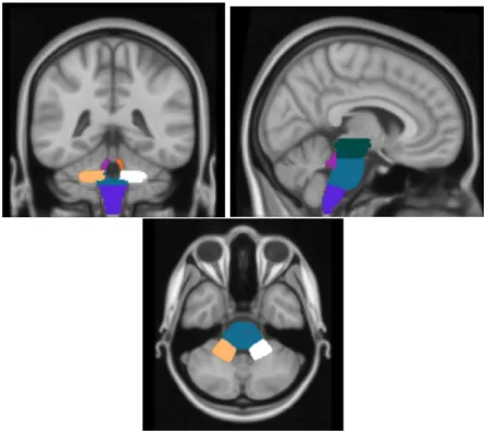
The ultimate goal of pre-processing steps is to evaluate the volumes of all brain regions that will be used to create the graph. A software called Freesurfer [42] is used to calculate the volume of brain regions. Using Freesurfer it is possible to get morphological information about supratentorial and infratentorial regions, but it returns an unique volume value for the whole brainstem region Figure 4.1. We were particularly interested in investigating regions of the brainstem because they are the most impaired in MSA. To do that seven brain regions (Midbrain, Pons, Medulla, Right-SCP, Left-SCP, Right-MCP, Left-MCP) included in the
brainstem were hand drawn on MNI atlas [43] and then registered on subject specific space to evaluate volumes.
Figure 4.1: Structures of the brainstem
4.3.1 Brain Extraction Tool (BET)
Every T1-w images were processed with Brain Extraction Tool (provided by FSL
[44]) in order to delate non-brain tissue from images of whole head. In Figure 4.2 it is shown how BET works on a brain image.
Figure 4.2: Example of BET
This is an obligatory step for the linear registration that will be applied. There were some subjects where BET did not work, so it was necessary to adjust parameters (-f and -g) to get the best results out. The -f option in BET is used to set a fractional intensity threshold which determines where the edge of the final segmented brain is located. The default value is 0.5 and the valid range is 0 to 1. A smaller value for this threshold will cause the segmented brain to be larger and should be used when the overall result from BET is too small (inside the brain boundary). Obviously, larger values for this threshold have the opposite effect (making the segmented brain smaller). The -g option in BET causes a gradient change to be applied to the previous threshold value. That is,
the value of the -f intensity threshold will vary from the top to the bottom of the image, centered around the value specified with the -f option. The default value for this gradient option is 0, and the valid range is -1 to +1. A positive value will cause the intensity threshold to be smaller at the bottom of the image and larger at the top of the image. This will have the effect of increasing the estimated brain size in the bottom slices and reducing it in the top slices.
In 25 cases BET worked successfully as it is shown in Figure 4.3. For 7 images we decided to use the skull remotion of Freesurfer using the command -<no>skullstrip. Unfortunately the registration of four brains did not work because the brain extraction in the cerebellum region was not good enough, so we decided to remove the entire cerebellum to do the registration. To do that we created a cerebellum mask (Figure 4.4) and than we subtracted it from the input image. This problem occurs because the fact that cerebellum of MSA patients, in particular MSA-C patient, is really atrophic and cause problems during registrations (Figure 4.5).
Figure 4.3: T1-w image of healthy control where BET procedure works
Figure 4.4: Cerebellum mask
Figure 4.5: Example of atrophic cerebellum in MSA-C patient
4.3.2 Lesion Filling (LF)
This process takes a user-defined lesion mask (created manually by a neurora-diologist on GIMP software [45]) on a structural image T2-weighted and then
registered on the 3D T1-w in order to "fill" the lesion area in the structural
image with intensities that are similar to those in the non-lesion neighborhood (restricted to white matter only). It has been shown [46] that using such a method as part of a pre-processing pipeline can improve the registration and segmentation of pathological brains and the resultant volumetric measures of brain tissue [47].
4.3.3 Freesurfer
Using the “recon-all” command in Freesurfer, 82 brain region were segmented (Figure 4.6) and volumes were evaluated for the entire dataset on T1-w images
or on T1-w images after lesion filling if it was present. At this point we want
to calculate the volume of the 7 different regions in the brainstem that are not segmented automatically by Freesurfer.
Figure 4.6: Freesurfer segmentation. From left to right: coronal, sagittal and axial view
4.3.4 Brainstem regions
To evaluate the volume of the seven brain regions included in the brainstem described before, a neuroradiologist drew them on the MNI and then all 3D T1-w images were registered on MNI (Figure 4.7). Registration algorithms can
be divided into linear and non-linear depending on the type of deformations they permit.
The first registration is a linear registration and for this step we used FLIRT (FMRIB’s Linear Image Registration Tool). Liner registration means that an image can translate, rotate, zoom and shear to match with another. It uses images without skull, that is why the BET process is so important. The main options are: an input -in (T1-w images after LF) and a reference -ref (MNI)
volume; the calculated affine transformation that registers the input to the reference which is saved as a 4x4 affine matrix omat; and the output volume -out which is the result obtained transforming the input volume to align with the reference image. For these usages the reference volume must still be specified as this sets the voxel and image dimensions of the resulting volume. For the registration we set 12 degrees of freedom.
The second registration is a non-linear registration, and for this step we used FNIRT (FMRIB’s Non-linear Image Registration Tool) that performs non-linear transformations like contraction and dilations in order to have a better registration of images on MNI.
Finally, the transformations were inverted so all the seven regions were reg-istered back on their specific space in order to evaluate their volumes.
Figure 4.7: Brainstem regions hand drawn. From the left to the right: coronal, sagittal and axial view
4.4 Construction of structural correlation network
4.4.1 Node decision
We wanted to create a graph for each group of subjects (MSA, Stridor, No-Stridor, Healthy Controls) and then compare them with a statistical analysis.
To do that our correlation matrices were constructed based on pair-wise correlations between ROI pairs (negative correlations were replaced with zero). The structural correlation between a ROI pair of i and j was defined as the Pear-son correlation coefficient between their mean GM volumes across the subjects within a group.
In order to obtain the volumes of ROIs it is necessary to choose a way to segment our 3D brain T1-w images in different regions. To obtain the ROIs
in our study we resorted to a specific software, Freesurfer [42], that works with complex segmentation algorithms. Freesurfer is an open source software suite for
processing and analyzing brain MRI images. We performed it for each subject and this allowed us to obtain regions subject-specific, this process takes about 12 hours (depending on the performance of the computer processor). We then obtained all the ROIs that Freesurfer was able to segment, and we chose 82 regions between these covering the entire cortex and deep grey matter. Since MSA disease produces particular changes in volume in brainstem regions, we were particularly interested to study these structures. To do this, some regions were hand drawn in the space of MNI. In particular seven brain regions were hand drawn (Midbrain, Pons, Medulla, Right-SCP, SCP, Right-MCP, Left-MCP). In Table 4.3 Table 4.4 and Table 4.5 subcortical and cortical ROIs are listed. All the regions, i.e. the future nodes, are associated with a number which will make the identification easier.
N ROI 1 Left-cerebellum-cortex 2 Left-thalamus-proper 3 Left-Caudate 4 Left-Putamen 5 Left-pallidum 6 Left-hippocampus 7 Left-amygdala 8 Left-accumbens-area 9 Right-cerebellum-cortex 10 Right-thalamus-proper 11 Right-caudate 12 Right-putamen 13 Right-pallidum 14 Right-hippocampus 15 Right-amygdala 16 Right-Accumbens-area 17 Left-superiorparietal 18 Left-caudalanteriorcingulate 19 Left-cuneus 20 Left-rostralanteriorcingulate 21 Left-isthmuscingulate 22 Left-pericalcarine 23 Left-transversetemporal 24 Left-caudalmiddlefrontal 25 Left-fusiform 26 Left-parstriangularis 27 Left-temporalpole 28 Left-postcentral 29 Left-superiortemporal 30 Left-middletemporal 31 Left-entorhinal 32 Left-rostralmiddlefrontal 33 Left-parsorbitalis 34 Left-inferiortemporal 35 Left-frontalpole 36 Left-posteriorcingulate 37 Left-medialorbitofrontal 38 Left-lateraloccipital 39 Left-paracentral 40 Left-parahippocampal 41 Left-insula 42 Left-supramarginal
N ROI 43 Left-lingual 44 Left-parsopercularis 45 Left-inferiorparietal 46 Left-precentral 47 Left-superiorfrontal 48 Left-lateralorbitofrontal 49 Left-precuneus 50 Right-superiorparietal 51 Right-caudalanteriorcingulate 52 Right-cuneus 53 Right-rostralanteriorcingulate 54 Right-isthmuscingulate 55 Right-pericalcarine 56 Right-transversetemporal 57 Right-caudalmiddlefrontal 58 Right-fusiform 59 Right-parstriangularis 60 Right-temporalpole 61 Right-postcentral 62 Right-superiortemporal 63 Right-middletemporal 64 Right-entorhinal 65 Right-rostralmiddlefrontal 66 Right-parsorbitalis 67 Right-inferiortemporal 68 Right-frontalpole 69 Right-posteriorcingulate 70 Right-medialorbitofrontal 71 Right-lateraloccipital 72 Right-paracentral 73 Right-parahippocampal 74 Right-insula 75 Right-supramarginal 76 Right-lingual 77 Right-parsopercularis 78 Right-inferiorparietal 79 Right-precentral 80 Right-superiorfrontal 81 Right-lateralorbitofrontal 82 Right-precuneus