ALMA MATER STUDIORUM - UNIVERSITÀ DI BOLOGNA
FACOLTA’ DI INGEGNERIA
CORSO DI LAUREA IN CIVIL ENGINEERING
DICAM– Dipartimento di Ingegneria Civile, Ambientale e dei Materiali
TESI DI LAUREA in
Advanced Design of Structures
FATIGUE LIFE ASSESSMENT OF A RAILWAY BRIDGE USIGN A DYNAMIC INTERACTION MODEL
CANDIDATO: RELATORE:
Rossi Fabrizio Prof. Ing. Marco Savoia
CORRELATORE: Prof. Ing. Loris Vincenzi
Anno Accademico 2010/11 Sessione III
Index
INTRODUCTION ... 1
1. BASIC OF DYNAMIC ... 5
1.1GENERAL REMARKS ... 5
1.2SINGLE DEGREE OF FREEDOM SYSTEM ... 6
1.3MULTI-DEGREE OF FREEDOM SYSTEM ... 9
1.4DAMPING IN STRUCTURES ... 12
2. METHODS FOR SOLVING THE EQUATIONS OF MOTION ... 15
2.1GENERAL OVERVIEW ... 15
2.2CLASSICAL MODAL ANALYSIS ... 16
2.3NUMERICAL TIME-STEPPING METHODS ... 18
3. MOVING LOADS MODEL ... 21
3.1INTRODUCTION ... 21
3.2SIMPLY-SUPPORTED BEAM SUBJECTED TO MOVING LOADS ... 22
3.3ASSUMPTION AND LIMITATION OF THE MODEL ... 24
4. VEHICLE-BRIDGE INTERACTION MODELS ... 25
4.1INTRODUCTION ... 25
4.2TRAIN SUBSYSTEM ... 26
4.3BRIDGE SUBSYSTEM ... 31
4.4COMPUTATION OF THE COUPLED TRAIN-BRIDGE SYSTEM ... 34
5. PONTELAGOSCURO RAILWAY BRIDGE ... 37
5.1DESCRIPTION OF THE BRIDGE ... 37
5.2EXPERIMENTAL DATA ... 44
5.3BRIDGE FINITE ELEMENTS MODEL ... 47
6. OPTIMIZATION PROCESS ... 51
6.1INTRODUCTION ... 51
6.2DIFFERENTIAL EVOLUTION ALGORITHM ... 52
6.3THE RESPONSE SURFACE METHOD ... 57
6.4DE ALGORITHM WITH A SECOND-ORDER APPROXIMATION ... 59
6.5OPTIMIZATION ALGORITHM APPLICATION ... 62
7. 2D MOVING LOADS VS. VBI MODELS APPLICATION ... 69
7.1INTRODUCTION ... 69
7.2BRIDGE MODEL SETTING ... 70
7.3TRAIN DATA ... 73
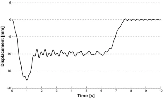
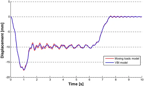
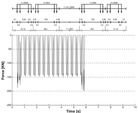
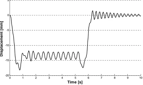
7.4COMPARISON BETWEEN MOVING LOADS MODEL AND VBI MODEL ... 79
7.5PARAMETERS INVESTIGATION ... 101
8. 3D VBI MODEL APPLICATION ... 105
8.1INTRODUCTION ... 105
8.2THREE-DIMENSIONAL DYNAMIC ANALYSES ... 106
9. FATIGUE ASSESSMENT ... 125
9.1GENERAL ... 125
9.2RAINFLOW CYCLE COUNTING ... 129
9.3PALMGREN-MINER RULE ... 131
9.4FATIGUE VERIFICATION ... 134
10. CONCLUSION AND FUTURE DEVELOPMENT ... 157
APPENDIX ... 161
1
INTRODUCTION
With the end of the second world war, there was the need of rebuilding the decaying infrastructures of the country, as the railway lines and the bridges. In this historical period the most used material that allowed to build long span bridges was the steel, since prestressed concrete was just born in those years. Along with steel, the riveted systems, was the technique used to connect among each other the elements of the metallic structures. Nowadays this technique has been overcome by welding and high strength bolts systems that offer benefits in terms of costs and realization velocity.
However the study of the riveted connections is still a current issue, especially for those engineers that deal with maintenance and retrofitting of existent structures. In fact many of the bridges built at that time are nowadays still used, although traffic volumes, loads and speed are changed during these years. Therefore the service loads, the accumulated stress cycles due to traffic and aging, have been induced to the evaluation of the remaining fatigue life of these structures and to operations of maintenance and replacement.
The “discovery” of fatigue occurred in the 1800s when several researchers in Europe observed that bridge and railroad components were cracking when subjected to repeated loading. As the century progressed and the use of metals expanded with the increasing use of machines, more and more failures of components subjected to repeated loads were recorded. By the mid 1800s A. Wohler proposed a method by which the failure of elements from repeated loads could be mitigated, and in some cases eliminated. This method resulted in the stress-life response diagram and element test model approach to fatigue design and verification.
2
The aim of this research is to assess the fatigue life of an existent metallic railway bridge. In particular the investigated structure is a bridge on the railway line Bologna-Padova that crossing the Po river between Pontelagoscuro and Occhiobello. It was built in the years from 1946 to 1949, and it is a truss system, where the elements are connected by means of rivets.
The standard procedure given by the guidelines and therefore used by the designer to carry out dynamic analyses of bridges is to model the vehicles as a sequence of moving loads. Actually in this study in order to achieve more accurate results according to what really happens in the real case, a train-bridge dynamic interaction model is first set up and then used to perform dynamic analyses of the structure.
The dynamic interaction between a bridge and the moving vehicles represents a special discipline within the broad area of structural dynamics. The vehicles considered may be those constituting the traffic flow of a highway bridge, in general, or those that form a connected line of railroad cars, in particular.
In order to simulate the train-bridge interactive dynamics many kinds of two-dimensional and three-two-dimensional models for train carriages have been presented and adopted, in which the springs and damping are used to describe the interactive effects between wheels and primary suspensions as well as primary and secondary suspensions. Therefore from the theoretical point of view, the two subsystems, the bridge and the moving vehicles, can be simulated as two elastic structures. The two subsystems interact with each other through the contact forces, the forces induced at the contact points between the wheels and the rails surface (of the railway bridge) or the pavement surface (of the highway bridge). Such a problem is nonlinear and time-dependent due to the fact that the contact forces may move from time to time, while their magnitudes do not remain constant, as a result of the relative movement of the two subsystems.
Therefore this paper proposes in the first chapter some basic notions of dynamic for the single degree of freedom and multi degree of freedom systems, focusing the attention on the eigenvalue problem by which it is possible to obtain the eigenmodes and frequencies of an elastic system.
Since no analytical solution is possible for this kind of problems, in the second chapter, two possible ways to solve the equations of motion are presented. It is also discussed that if the system has classical damping, classical modal analysis can be used to uncoupled the equations of motion, otherwise numerical time-stepping methods are
3 needed. In this research only the Newmark’s method is presented, because it is indeed the method used.
In the third chapter the classical way to represent a vehicle travelling on a bridge is presented. Usually this is done by means of a sequence of moving loads. This method is also the one proposed by the Eurocode 1 [1] to carry out dynamic analysis of bridges, and it is the widespread method used by the researchers.
In the fourth chapter, other methods to model a vehicle crossing are discussed. These methods consider the dynamic interaction between the vehicle and the bridge. In this way the vehicle and the bridge are considered as two systems that exchange each other the interaction forces caused by the relative motion. Generally this problem is described by two sets of equations, one for the bridge and one for the vehicle, coupled by interactions conditions. It is shown that the solution can be obtained different methods, subdivided into two different group, which are iterative and non-iterative.
In the fifth chapter the railway bridge investigated is presented in details, not only in terms of material, geometry and structural topology, but also as regards the dynamic behavior of the structure. In fact from experimental modal analysis, natural frequencies and mode shapes are known. Furthermore the finite element model to perform the dynamic analyses is discussed.
Once the bridge has been modeled, in chapter six, an optimization algorithm is used to adjust the model to have modal parameters as closed as possible to the measured data. Therefore the Differential Evolution Algorithm used to solve the optimization problem of the significant mechanical parameters is described in detail, and the obtained results are presented.
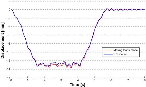
Then in the seventh chapter a comparison between the moving loads and the vehicle-bridge interaction models is done, using an equivalent two dimensional model of the Pontelagoscuro bridge. Actually two dimensional analyses of the bridge are carried out using the trains models given by the Eurocode 1 for fatigue analyses, and as regard VBI analyses the data regarding the suspensions system of the train ETR 500Y [2], [3] have been used. Then the results obtained are compared with those obtained by another author [4], which has carry out dynamic analyses of the same bridge using the Eurocode 1 approach, which is the moving loads method.
4
In chapter eight, three dimensional dynamic analyses of the bridge are computed using a more sophisticated 3D train model, used to involve and to take into account also lateral and torsional mode shapes of the structure.
Chapter nine is completely devoted to the assessment of the fatigue life of the bridge. First of all basic notion of fatigue theory are given along with the cycles counting Rainflow method used to reduce a spectrum of varying stress into a set of simple stress reversals, and Miner rule used to quantify the damage in the elements. Then the results obtained for the studied case are discussed and the critical elements that could be subjected to fatigue problem are identified using two different approaches, which are the Eurocode [5], and another method proposed by L. Georgiev [6].
In chapter ten, some conclusions and some proposal for future development are suggested.
5
1. BASIC OF DYNAMIC
1.1 General remarks
Any structure, or in general a system, may be described as a set of interconnected elements, that are able to react with the surrounding environment. The structure’s behavior is studied through the use of suitable models able to simplify the real problem, which in general can be very complex. The models are appropriate only if the consequences derived from the assumptions are in agreement with the experimental results.
In studying the dynamic problem of a structure, continuous or discrete models can be used. Continuous systems have infinite number of degrees of freedom, in fact a generic configuration is fixed by infinite number of parameters or coordinates. The dynamic behavior of a continuous system is described by partial differential equations as the parameters defining the motion of the system depend both on time and space. A closed form solution is obtainable only in the particular case in which the mass and the elastic proprieties are uniformly distributed. This approach is rarely feasible if the flexural rigidity or mass varies along the length of the beam, if complex constraint conditions are involved, or if the system is an assemblage of several members with distributed mass.
Discrete systems, instead, have a finite number of degrees of freedom, and the system’s configuration is described by parameters that are only function of time. Therefore the differential equations of such systems are ordinary differential equations. However discrete systems can effectively idealize many classes of structures. Moreover effective methods that are ideal for computer implementation are available to solve the system of ordinary differential equations governing the motion of such systems.
6
1.2 Single degree of freedom system
Some structures, such as an elevated water tank or one-story frame structure or two-span bridge supported by a single column of figure (1.1), could be idealized as a concentrated mass supported by a massless stem with stiffness , when interested in understanding the structural dynamic in the horizontal direction.
In those models the number of independents displacements required to define the displaced positions of all the masses relative to their original position is just one. For that reason they are called single degree of freedom system (SDOF).
In a real structure each structural member (beam, column, wall, etc.) contributes to the inertial (mass), elastic (stiffness or flexibility), and energy dissipation (damping) properties of the structure. In the idealized system represented in figure (1.2), however, each of these properties is concentrated in three separate, pure components: mass component, stiffness component, and damping component.
Figure 1.1: Example of SDOF structures: (a) Water tank supported by single column; (b) one-story frame
building; (c) two-span bridge supported by single comlumn; (d) induced motion of a SDOF.
(a) (b) (c) (d)
(a) (b)
7 Therefore the response of a structure depends on its mass, stiffness, damping, and
applied load or displacements. By applying Newton’s law and D’Alembert’s principle
of dynamic equilibrium, it can be shown that
(1.1)
where is the inertial force of the single mass and is related to the acceleration of the mass
by ; is the damping force on the mass and related to the velocity across the
viscous damper by ; is the elastic force exerted on the mass and related to the
relative displacement between the mass and the ground by , where is the spring
constant; is the damping ratio; and is the mass of the dynamic system. Substituting these expression for , , and into Eq. (1.1) gives
(1.2)
The above equation of motion of a SDOF can be solved in closed form only for excitations that can be described analytically. If the excitation varies arbitrarily with time, closed form solution doesn’t exist, and the equation can be solved by numerical time-step method.
The characteristics of the oscillations such as the time to complete one cycle of
oscillation and the number of oscillation cycles per second are intrinsic
properties of the system, and do not depend on the external applied force. Dividing the Equation (1.2) specialized for free vibration (right term equal to zero) by its mass will result in
2 0 (1.3)
where ⁄ the natural frequency of vibration of the undamped frequency;
⁄ the damping ratio; 2 2√ 2 / the critical damping
coefficient. The time required for the SDOF system to complete one cycle of vibration is called the natural period of vibration of the system and is given by
2
2 (1.4)
Furthermore, the natural cyclic frequency of vibration is given by
2 1
8
The circular frequency of the vibration or the damped vibration frequency of the
SDOF structure, , is given by √1 .
The damped period of vibration ( of the system is given by
2 2
√1 (1.6)
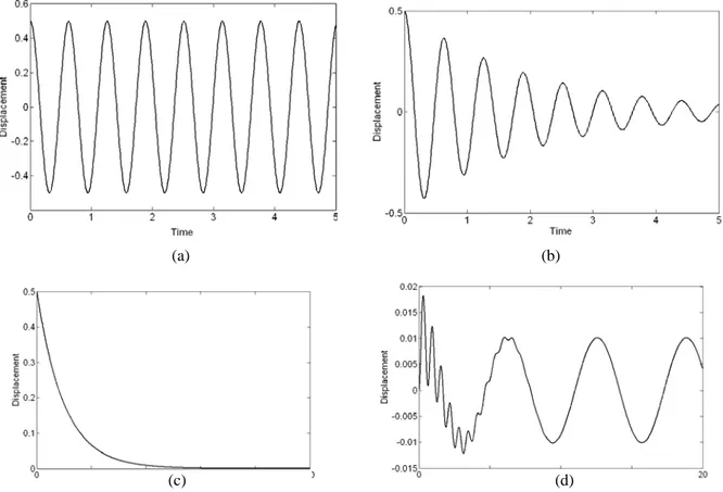
When 1 or the structure returns to its equilibrium position without
oscillating and is referred to as a critically damped structure. When 1 or , the
structure is overdamped and comes to rest without oscillating, but at a slower rate. When
1 or , the structure is underdumped and oscillates about its equilibrium state
with progressively decreasing amplitude, see figure (1.3).
For structure such as buildings, bridges, dams, and offshore structures, the damping ratio is less than 0.15 and thus can be categorized as underdumped structure. So the basic dynamic properties estimated using damped or undumped assumptions are approximately the same. Thus, the damping coefficient accounts for all energy-dissipating mechanisms of the structure and can be estimated only by experimental methods.
Figure 1.3: Example of SDOF systems responses: (a) Undamped free vibration; (b) Underdamped free
vibration; (c) Overdamped free vibration; (d) Damped armonic forced vibration. (a) (b)
9
1.3 Multi-degree of freedom system
The SDOF approach may not be applicable for complex structures such as multilevel frame structures and bridges with several supports. To predict the response of a complex structure, the structure is discretized with several members of lumped masses. As the number of lumped masses increases, the number of displacements required to define the displaced positions of all masses increases.
The equation of motion, of a multi-degree of freedom (MDOF) system represented in figure (1.4), is similar to that relative to the SDOF system, but the stiffness , mass , and damping are matrices.
The most general equation of motion of an MDOF system can be written as
(1.7)
The stiffness matrix can be obtained from standard static displacement-based
analysis models and may have off-diagonal terms. The mass matrix due to the negligible
effect of mass coupling can best be expressed in the form of tributary lumped masses to the corresponding displacement degree of freedoms, resulting in a diagonal or uncoupled mass matrix. The damping matrix accounts for all the energy-dissipating mechanisms in the structure and may have off-diagonal terms. The right term is the vector of the external forces acting on each degree of freedom.
To better understand the response of MDOF systems, we look first at the undamped, free vibrations. By setting and to zero in the Eq. (1.7), the equation of motion of an
N-DOF system can be shown as:
0 (1.8)
where and are square matrices.
10
The signal of a natural vibration mode can be described mathematically by:
(1.9)
Where is the deflected shape of the structure, and the harmonic function describes the
time variation of the displacement and constants determined using the initial
conditions of the motion. Combining and simplifying equation (1.8) and (1.9) gives the eigenvalue problem, which is used to determine the eigenvector corresponding to the natural mode shapes, , and natural frequencies, , of the structure.
0 (1.10)
The N eigenvectors can be assembled in a single square modal matrix .
One of the important aspects of these mode shapes is that they are orthogonal to each other. This lead to
∗ (1.11)
∗ (1.12)
where ∗ and ∗ are diagonal matrices.
When damping of the MDOF system is included, the free vibration response of the damped system will be given by
0 (1.13)
The displacements are first expressed in terms of natural mode shapes, and later they are multiplied by the transformed natural mode matrix to obtain the following expression:
∗ ∗ ∗ 0 (1.14)
where, ∗ and ∗ are diagonal matrices given by Eqs. (1.11) and (1.12) and
∗ (1.15)
While ∗ and ∗ are diagonal matrices, ∗ may have off-diagonal terms. When has
off diagonal terms, the damping matrix is referred to as a nonclassical or nonproportional damping matrix. When is diagonal, it is referred to as a classical or proportional damping matrix. Classical damping is an appropriate idealization when similar damping mechanisms are distributed throughout the structure. Nonclassical damping idealization is appropriate for the analysis when the damping mechanisms differ considerably within a structural system. Since most civil structures have predominantly one type of construction
11 material, they could be idealized as a classical damping structural system. Thus, the damping matrix of Eq. (1.16) will be a diagonal matrix. Therefore the equation of th
mode shape or generalized h modal equation is given by
2 0 (1.16)
Equation (1.16) is similar to the Eq. (1.3) of an SDOF system. Also, the vibration properties of each mode can be determined by solving the Eq. (1.16).
Methods for solving the equations of motions (1.3) or (1.17) and (1.7) are developed in detail in chapter 2.
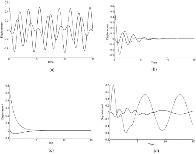
In figure (2.5) the responses of some possible two degrees of freedom systems are shown.
(a)
Figure 2.5: Example of 2-DOFs systems responses: (a) Undamped free vibration; (b) Underdamped free
vibration; (c) Overdamped free vibration; (d) Damped armonic forced vibration. (b)
12
1.4 Damping in structures
The damping of a structure is related to the amount of energy dissipated during its motion. It could be assumed that a portion of the energy is lost due to the deformations, and thus damping could be idealized as proportional to the stiffness of the structure. Another mechanism of energy dissipation could be attributed to the mass of the structure, and thus damping idealized as proportional to the mass of the structure. In Rayleigh damping, it is assumed that the damping is proportional to the mass and stiffness of the structure.
(1.17)
The generalized damping of the th mode is then given by
(1.18)
(1.19)
knowing that
2 (1.20)
therefore substituting Eq. (1.19) in (1.20) and simplifying results in
2 2 (1.21)
13
The coefficients and can be determined from specified damping ratios at two
independent dominant modes (say, iand jmodes). In figure (1.6) the Rayleigh damping
variation with natural frequency is shown.
Expressing Eq. (1.21) for these two modes will lead to the following equations:
2 2 (1.22)
2 2 (1.23)
When the damping ratio at both the i and j modes is the same and equals , it can be shown that
2
(1.24)
2
(1.25)
It is important to note that the damping ratio at a mode between the ithand jthmode is less than . And, in practical problems the specified damping ratios should be chosen to ensure reasonable values in all the mode shapes that lie between the ith and jth mode shapes.
15
2. METHODS FOR SOLVING THE
EQUATIONS OF MOTION
2.1 General overview
The dynamic response of linear systems with classical damping that is a reasonable model for many structures can be determined by classical modal analysis. Classical natural frequency and modes of vibration exist for such systems, and their equations of motion, when transformed to modal coordinates, become uncoupled (chapter 1.3). Thus the response in each natural vibration mode can be computed independently of the others, and modal response can be combined to determine the total response. Each mode responds with its own particular pattern of deformation, the mode shape, with its own frequency, the natural frequency, and with its own damping. Each modal response can be computed as a function of time by analysis of a SDOF system with the vibration properties of the particular mode. These SDOF equations can be solved in closed form for excitations that can be described analytically, or they can be solved by time stepping methods for complicated excitations.
For systems with nonclassical damping the equations of motion cannot be uncoupled by transforming to modal coordinates of the system without damping. Therefore such systems can be analyzed by direct solutions of the coupled system of differential equations. This approach requires numerical methods because closed-form analytical solutions are not possible even if the dynamic excitation is a simple function described analytically.
16
2.2 Classical modal analysis
For MDOF systems, the general form of the equations of motion are given by Eq. (1.7) repeated here for convenience:
which in modal coordinates can be rewritten as
∗ ∗ ∗ ∗ (2.1)
where ∗, ∗ and ∗ are already introduced in Eq. (1.11) (1.12) and (1.15), while the right term is given by
∗ (2.2)
The expression (2.1) represents a set of uncoupled equations in modal coordinates , if the system has classical damping. For such systems, the generic equation can be written as
∗ ∗ ∗ ∗ (2.3)
This equation governs the response of the SDOF. Dividing Eq. (2.3) by ∗ gives
2 ∗ ∗ (2.4)
Thus we have uncoupled equations like Eq. (2.3) or (2.4) one for each natural mode. In summary, the set of coupled differential equations (2.1) in nodal displacements
has been transformed to the set of uncoupled equations (2.3) in modal coordinates .
As already mentioned each modal equation is of the same form as the equation of motion of a SDOF system. Thus solution methods and results available for SDOF systems
can be adapted to obtain solutions for the modal equations. So if the external forces
are analytical functions, closed-form solutions are available, otherwise numerical methods
are needed (chapter 2.3). Once is established, the displacement due to the mode
will be given by . The total displacement due to combination of all
mode shapes can then be determined by summing up all displacements for each mode, and is given by
17 This procedure is known as classical modal analysis or the classical superposition
method because individual modal equations are solved to determine the modal coordinates
.
This analysis method is restricted to linear systems with classical damping. Linearity of the system is implicit in using the principle of superposition. Damping must be of the classical form in order to obtain modal equations that are uncoupled, a central feature of modal analysis.
It is shown that for MDOF system, the equations of motion can be transformed in modal coordinates to obtain Eq. (2.1). But this transformation is not advantageous when dealing with systems with many degrees of freedom excited by complicated expressions of the external forces. In fact in these cases solving coupled equation of the type (1.7) or equations of the type (2.3) is almost the same, because in both cases a numerical time-stepping method is needed.
Actually for many practical problems only the few first modes contribute significantly to the response. This means that for systems with classical or nonclassical damping it is necessary to solve the uncoupled modal equations for only the significant modes. If only the first J modes contribute significantly to the response, the size of Eq.
(3.1) can be reduced accordingly; is now an J matrix; ∗, ∗ and ∗ are J J
matrices; and ∗ is a J 1 vector. Thus the problem reduces to solving these J
uncoupled equations for , 1,2, … , J with a numerical method. Once have
been determined at each time instant, is computed from Eq. (2.5) with its summation
18
2.3 Numerical time-stepping methods
A vast body of literature exists about numerical time-stepping methods for integration of differential equations. However in this section only the Newmark’s method is treated as, with appropriate choices of the parameters this scheme ensures convergence, stability and accuracy. The method is developed for the equation of motion of the SDOF, however the extension to the equations of the MDOF is straightforward.
In 1959, N. M. Newmark developed a family of time-stepping methods based on the following equations:
1 ∆ ∆ (2.6.a)
∆ 0.5 ∆ ∆ (2.6.b)
Typical selection for is 1/2 and 1/4 is satisfactory from all points of view,
including that of accuracy, as it possible to see in figure (2.1). For linear systems these two equations, combined with the equilibrium equation
(2.7)
at the end of time step, provide the basis for computing , and from the
known , and at time . Defining the following quantities
∆ ∆ ∆ (2.8)
∆ (2.9)
the Eq. (2.6) can be rewritten as
∆ ∆ ∆ ∆ (2.10.a)
∆ ∆ ∆
2 ∆ ∆ (2.10.b)
The Eq. (2.10.b) can be solved for ∆ and substituted in the Eq. (2.10.a). The two expression just founded are then substituted in the incremental equation of motion
∆ ∆ ∆ ∆ (2.11)
This substitution gives
∆ ∆ ̂ (2.12)
19 ∆ 1 ∆ (2.13) and ∆ ̂ ∆ 1 ∆ 1 2 ∆ 2 1 (2.14)
With and ∆ ̂ known from the system properties , and , algorithm parameters and , and the and at the beginning of the time step, the incremental displacement is computed from
∆ ∆ ̂ (2.15)
Once ∆ is known ∆ and ∆ can be computed from Eqs. (2.10.a) and (2.10.b) then
, and from Eq. (2.8). The acceleration can also be obtained from the
equation of motion :
(2.16)
Actually Eq. (2.16) is needed to obtain to start the computations.
This procedure can readily be extended to MDOF systems. The scalar equations (2.10.a) and (2.10.b) that relate the response (displacement, velocity, and acceleration) increments over time step to 1 to each other and the response values at time , and the scalar equation (2.11) of incremental equilibrium, all now become matrix equations.
21
3. MOVING LOADS MODEL
3.1 Introduction
The simplest case that can be conceived of a moving vehicle is when it is represented as concentrated loads. This is the so called moving loads model.
The most basic problem in the study of vehicle-induced vibrations on bridges is the dynamic response of a simply-supported beam subjected to a single moving load. This problem is important in that the solution can be given in closed form. By the principle of superposition the solution obtained for a single moving load could be expanded to deal with a series of identical equi-distant moving loads. Research on the vibration of bridges traveled by moving loads is abundant. The most related ones are the works by Timoshenko [7] and Fryba [8].
In the dynamic analysis of a railway bridge, a moving train is traditionally represented as a series of moving axle loads. This approach is the one adopted by many researchers and also by many design codes, as for example the Eurocode 1. With this model, the global dynamic characteristics of the bridge caused by the moving action of the vehicle can be captured with a sufficient degree of accuracy. However, the effect of interaction between the bridge and the moving load is ignored. For this reason, the moving load model is good only for the case where the mass of the vehicle is small relative to that of the bridge, and only when the vehicle response is not of interest.
In this section the moving loads model will be treaty in a general way within the
framework of the finite elements method, leaving the reader who is interested in
22
3.2 Simply-supported beam subjected to moving loads
In this section, the general method to perform a dynamic analysis of railway bridges subjected to moving loads is given by means of reduced model of train bridges. The problem is illustrated in figure (3.1).
The model is based on the fact that the fundamental dynamic behavior of certain type of bridges may be described by the dynamic behavior of two-dimensional Bernoulli beams. The Bernoulli beam is modeled using several numbers of beam elements. A schematic illustration of the transformation of a railway bridge to a beam element model is shown in Figure (3.2). However, the whole following procedure is easily extended also to three-dimensional models, if more sophisticated analyses are needed.
The model can be implemented given as input the properties of the beam elements such as the damping value, Young's modulus, moment of inertia and mass per unit length. Then the following steps could be performed in order to set-up the bridge model:
- Creating the matrices , and for a 2D elastic Bernoulli beam element.
- Assemble the element matrices , and in the global matrices , and .
Figure 3.1: Moving loads model.
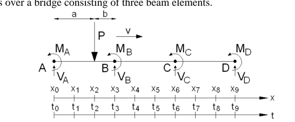
23 After that the load vector has to be constructed. Figure (3.3) illustrates a point load that moves over a bridge consisting of three beam elements.
The force moves with the velocity between and over the nodes of the model. In a finite elements model all loads are applied at the element nodes. The load is therefore assigned as equivalent nodal forces, when is situated between the nodes of a beam element. The equivalent shear forces and moments are computed as:
1 2 (3.1)
(3.2)
1 2 (3.3)
(3.4)
In this way a matrix can be generated which describes the load history at each
node of the model for the whole time period of the analysis. The matrix is constructed by calculating the equivalent node loads using Eqs. (3.1)-(3.4) every time the load moves a distance ∆ . The size of the distance depends on the velocity and the size of a time step ∆ according to:
∆ ∙ ∆ (3.5)
After constructing the , , and matrices the dynamic responses in the bridge
could be calculated by solving the equations of motion (1.7). This can performed by using Newmark’s time-step method, described in chapter 2.3.
24
3.3 Assumption and limitation of the model
Actually two-dimensional beam models can only calculate vertical bending modes. A key assumption in this model is that vertical modes of vibration contributes to the vertical accelerations of the bridge, which implies that it is assumed that accurate results may be achieved even though torsional and horizontal bending modes are neglected. This is a limitation of the model since all bridges have torsional bending modes and, if they are excited, they often increase the vertically acceleration of the bridge. Torsional bending modes are mainly excited when a bridge is subjected to eccentric dynamic loads, as on two-rail bridges, and the reduced model is therefore more accurate for bridges with a centric track.
Also it must be ensure that the frequencies and shapes of the modes that are calculated using the reduced model are nearly the same as the frequency and eigenmodes of the real bridge.
In this procedure the bridge is modeled using Bernoulli beams, which implies that shear deformation is neglected. When modeling truss bridges shear deformations cannot be neglected. Therefore, the reduced model introduces more approximations when truss bridges are considered.
Another limitation of the model is that the beams all have the same properties. To make benefit of the result using the reduced model, it may be limited to railway bridges that have constant stiffness and weight along the length.
A last assumption is that columns and foundations were assumed to have a neglected vertical deformation and are therefore modeled as simple supports.
Actually all this assumptions and limitations can be easily overcome with some devices. In fact as already sad the model could be expanded in a three-dimensional model for instance, in order to have more sophisticated model, and models which take into account shear deformation can be built up. Therefore the bridge can be modeled in a finite elements software and performing a dynamic analysis assigning the load history at each node of the track.
25
4. VEHICLE-BRIDGE
INTERACTION
MODELS
4.1 Introduction
The dynamic response of railway bridges under moving trains has been a topic of research interest for many years, especially in last decades that has seen a worldwide development of high-speed railways.
In chapter 3 the problem of a train passing over a bridge it is treated as a sequence of travelling loads.
Considerable experimental and theoretical research has recently been performed on train-bridge interaction. For this aim different vehicle models with different degree of sophistication have been developed to account for the dynamic properties of the vehicle. The simplest model for a train is a series of 1 degree-of-freedom (DOF) mass–spring– damper systems that account for the suspension of the vehicle. Liu et al. [2] studied train– bridge interaction with a 3-DOF vehicle model consisting of the car body and wheel–axle sets and proposed a 15-DOF vehicle model and analyzed the passage of the ETR 500Y high speed train on the Sesia viaduct [10].
In this section a review of this models and methods, for solve the train-bridge dynamic interaction problem, are given.
26
4.2 Train subsystem
Vehicle model with a varying degree of sophistication can be found in literature to account for the dynamic effect of the train on the bridge. Possible planar models consisting in masses supported by springs and dashpots that could be used in the two-dimensional analyses are those represented in figure (4.1). The simplest model in this case is a SDOF moving mass supported by spring-dashpot unit, the so called sprung mass model (figure (4.1 a)). Vehicle model (c) consist in a car body, assumed to be rigid, resting on the front and rear bogies, each of which in turn is supported by two wheel sets; while vehicle (b) is an intermediate model.
In order to study the train-bridge interaction, a train composed of a sequence of one of the three models just presented can be used.
In a similar way as for the bridge, the equation of motion of the vehicle can be rewritten as
(4.1)
where , and , are the mass, damping and stiffness matrices; , and are the
displacement, velocity and acceleration vectors of the vehicle system; and is the force vector that collects the dynamic force on the vehicle. Without loss of generality, the terms in Eq. (4.1) specialized for the vehicle model (c) are given in the following. The mass matrix of the vehicle can be expressed as
0 0
0 0
0 0 (4.2)
(a) (b) (c)
Figure 4.1: (a) a 1-DOF (b) a 2-DOF and (c) a 3-DOF vehicle models for dynamic train-bridge interaction
27
where and are the mass of the bogie and the car body, respectively.
The stiffness matrix of the vehicle system is expressed as
2 0
2
0 2 (4.3)
where and are the spring stiffness coefficients of the primary and secondary
suspension system, respectively.
The damping matrix can be derived from the stiffness matrix by replacing the
stiffness coefficients ( , ) by the damping coefficients ( , ) of the primary and
secondary suspension system obtaining
2 0
2
0 2 (4.4)
The displacement, velocity and acceleration vectors , and are expressed as
(4.5)
(4.6)
(4.7)
where the subscript 1 and 3 indicate the vertical displacement, velocity and acceleration of the front and back bogie, respectively, while with the subscript 2 those of the car body.
The force vector is expressed in terms of the displacements and velocities of the wheel sets as follow
0 (4.8)
where and (with 1,2,3,4 represent the displacement and velocity of the th
wheel set, respectively.
More sophisticated three-dimensional models are available in order to perform more accurate train-bridge dynamic analyses [3]; a possible model is showed in figure (4.2). The equation of motion of this kind of model can still be represented by the Eq. (4.1). In this model the bogies and the wheel sets are linked by horizontal and vertical springs and
dampers. There are horizontal and vertical springs ( , ) and dampers ( , ) at each
28
) at each side of each bogie. Each car body and each bogie has 5 DOFs: the displacement in vertical direction ( ) and longitudinal direction ( ), and rotations around
the -axis ( ), -axis ( ) and -axis ( ). Each wheel set has 3 DOFs: the displacement
in vertical direction ( ) and longitudinal direction ( ), and rotation around the -axis ( ). In this way, the vehicle model has a degree of 27 DOFs.
The displacement as well as the velocity and acceleration vectors of the Eq. (4.1), of this model vehicle, assume the following form
, , , , , , , , , , , , , , (4.9)
where subscript 1 stands for the front bogie, subscript 2 stands for the car body, and subscript 3 stands for the rear bogie. The mass matrix of the vehicle system is given by
, , , , , , , , , , , , , , (4.10)
where is the mass of the bogie, , , are the mass moments of inertia of the bogie
around the -axis, -axis and -axis; with the subscript 2 are indicated the same quantities
for the car body is the mass of the car body, , , are the mass moments of inertia
of car body around the -axis, -axis and -axis. The stiffness matrix of the vehicle system is expressed as [10]:
29 (4.11) where 4 2 4 2 0 4 2 4 4 2 2 0 0 0 4 4 2 0 0 4 2 2 0 2 2 2 0 2 2 0 4 4 0 4 4 4 0 0 0 4 2 0 2 0 4 0 0 4 2 2 2 2 2 2 2 0 0 0 4 2 4 2 0 4 2 4 4 2 2 0 0 0 4
30
2 2
0 0
4 2 0
0 4
Where the meaning of all the terms that appears in the above matrices is specified in the figure (4.2).
Also in this case the damping matrix can be derived from the stiffness matrix
replacing the stiffness coefficients ( , , , ) by damping coefficients ( , ,
, ), in which and are vertical and horizontal damping coefficients at each side
of bogie in the first suspension system, and are vertical and horizontal damping
coefficients at each side of car body in the second suspension system.
The terms of the vector that are the interaction forces transferred to the bogies by the first suspension system can be expressed in terms of the displacements and velocities of the wheel sets as
2 2 2 2 2 2 2 2 2 2 0 0 0 0 0 2 2 2 2 2 2 2 2 2 2 (4.12)
31
4.3 Bridge subsystem
As shown in chapter 3, when a finite element model of the bridge is used to study its dynamic behavior, the equation of motion of the bridge can be expressed as
(4.13)
where , and are the mass matrix, damping matrix and stiffness matrix of the
bridge, respectively; , and represent the displacement, velocity and acceleration
vectors of the bridge DOFs; and is the force vector transferred to the bridge.
In some finite element model thousands of nodes and elements are used, therefore the Eq. (4.13) could be a system of thousands equations. Due to the fact that it is often possible to describe an approximate dynamic response with just a few eigenmodes the system equations can often be substantially reduced. In large finite element models a reduction of the system equations saves a lot of computer time. However, excluding modes is a crucial action. It is necessary to select the eigenmodes that have the largest influence on the result. This could be done using the modal superposition methods assuming that
only the first modes of the bridge are contributing to the response. The equation of
motion of the bridge can be now rewritten as follow:
∗ ∗ ∗ (4.14)
where it has been assumed that the eigenvectors are normalized with respect to the mass
matrix . The vector collects the modal coordinates. The matrices ∗, ∗ and the
vector ∗ are defined as follows:
∗ 2
∗ ∗
where is the matrix of eigenvectors and is the diagonal matrix of
eigenvalues of the considered modes.
As regard , it is determined by position, movement status and mass of the wheel
sets. As described in chapter 3.2 knowing the position of the th axle of the train it is possible to obtain the nodal forces vector by applying the Eqs. (3.1)-(3.4). Actually is composed of two terms, refers to the quasi-static part of the force that is related to the
32
33
When considering a 3-DOF vehicle model of figure (4.3) the force transferred to
the bridge can be written as
(4.15)
where represents the acceleration of the th wheel set; and represent the mass
and the axle load of the th wheel set, respectively, and 1| , , 3| , represents the
displacement of the bogie, which is related to the first and second wheel axle displacement when considering the first boogie and to the third and fourth wheel axle displacement when considering the second boogie. The vector is the 1 vector that transfers a moving unit load to nodal loads according to the position of the th axle.
34
4.4 Computation of the coupled train-bridge system
In studying the dynamic response of the vehicle-bridge interaction system, two sets of equations of motion can be written, one for the bridge Eq. (4.13) and the other for the vehicles Eq. (4.1). It is the interaction or contact forces existing at the contact points of the two subsystems that make the two sets of equations coupled. The algorithms to carry out this calculation can be classified in two main groups: (a) those based on an uncoupled
iterative procedure and (b) those based on the solution of the coupled system.
Algorithms based on an uncoupled iterative procedure treat the equations of motion of the vehicle and the bridge as two subsystems and solve them separately using a direct integration scheme. The compatibility conditions and equilibrium equations at the interface between the vehicle wheels and railway track are satisfied by an iterative procedure. One possible algorithm is illustrated in figure (4.4). In the first step of the iterative procedure,
the bridge response given by the Eq. (4.13) is computed with only , because the vehicle
is no yet excited. Assuming that there is no jumping between the wheels and the railway track, the wheels displacements and velocities can be computed, knowing the nodal displacements and velocities of the bridge, using the following beam shape functions
1 3 2 (4.16)
3 2 (4.17)
2 (4.18)
(4.19)
where represents the generic position of the th axle in between two successive nodes of the bridge. Then the right term of Eq. (4.1) can be computed and Eq. (4.1) can be solved for the displacement, velocity and acceleration of the vehicle DOFs. Then Eq. (4.13) is
solved again considering also , obtaining the bridge response. This procedure is
repeated for a number of iterations at each time step, until some convergence criterion is met (for example, until the difference between the bridge deflection of two successive iterations is sufficiently small).
35 Algorithms based on the solution of the coupled system are based on the solution of a unique system matrix at each point in time. The system matrix changes as the vehicle moves and is time-dependent. This procedure can be carried without any iteration solving the system given below for example with Newmark method
(4.20) Figure 4.4: Flowchart of the iterative solution procedure [3].
36
where , , and are coupled matrices attributed to the interaction between
the bridge and train. More details of this method are given in [11] and [12].
An alternative approach that leads to considerable savings in computational time is to implement the interaction on an element level rather than on a global level [9]. An interaction element is defined as that bridge element in contact with a vehicle wheel. Those bridge elements that are not directly under the action of vehicle wheels remain unaltered in the global matrixes of the system. The interaction element is characterized by two sets of equations: those of the bridge element and those of the moving vehicle above the bridge element. The DOFs of the moving vehicle can be solved in time domain using Newmark method, and then, the DOFs of the vehicle that are not in direct contact with the bridge are eliminated and condensed to the DOFs of the associated bridge element via the method of dynamic condensation. The interaction element has the same number of DOFs as the original bridge element and it can be directly assembled with the other bridge elements into the global matrix, while retaining symmetry property that is lost when condensation takes place on a global level.
37
5. PONTELAGOSCURO
RAILWAY
BRIDGE
5.1 Description of the bridge
In this section a brief description of the structure that will be used to carry out the dynamic analyses is given.
The structure considered is the steel bridge on the Bologna-Padova railway line that crosses the Po river and connects the areas of Pontelagoscuro and Occhiobello nearby Ferrara and Rovigo, respectively.
38
The Bologna-Padova railway line is an important link between the Nord-East area of Italy and the Nord-South national line Milano-Roma. For this reason in recent years significant infrastructural and technological investments have been planned upon this railway line in order to supply the transport demand in terms of passengers and freight trains.
The viaduct is composed of 9 truss girder bridges; the total length is about 610 m; seven 75.60 m long bridges compose the inner part of the viaduct, while two 59.4 m long bridges are located at the ends of the viaduct. The longest bridges are 9.60 m high, it is composed by 7 panels of 10.80 m. The shorter bridge is composed by 6 panels of 9.90 m and it is 7.50 m high.; in the following, all the analyses will performed with reference to only this kind of structure.
39 The bridge and each of its element was realized by connecting different kinds of hot-rolled profiles, obtained by the combination of thin plates with variable geometry along with L and I cross section shape elements.
The structure is composed by two main truss girders oriented in the longitudinal direction connected by transversal elements which form a closed cage sections as in figure (5.4).
Figure 5.3: Lateral span bridge view.
40
The truss girders are delimited at the top by an upper chord which are obtained combining by means of rivets four plates with four L angular profiles forming a box shaped beam as in figure (5.5).
This kind of cross section shape allows easy connections between elements and it guarantees an high moment of inertia in both directions in order to prevent instability phenomena.
In the lower part the vertical trusses are delimited by a lower chord, shown in figure (5.6) that are very similar to the upper chord
Then the upper and lower chords are linked together by vertical and diagonal elements.
The diagonal elements, as it is possible to see in figure (5.7), have a cross section composed by four L-shaped profile connected by means of plates. Actually it can be
Figure 5.5: Detail of the upper chords.
41 distinguished different kinds of diagonal elements, in fact the outer diagonals have connecting plates along all the length of the elements, instead the inner diagonals have connecting plates at regular intervals.
The vertical elements exhibit a double T cross section made by L profile coupled two by two and connected by means of plates as in figure (5.8). Also in this case there is difference between the outer vertical elements, which have a full web, and the inner ones which have lightened web done by plates at regular intervals.
Figure 5.7: Detail of the diagonal elements.
42
As already said in the upper and lower zone, there are struts and floor beams, respectively, which connect the truss girders, in order to create a closed box-shaped profile. There are struts and floor beams each 4.95 meters, in this way transversal elements and web elements are connected at the same time at the same node. The struts are consisting of two angular profile coupled two by two, with a web consisting of plates riveted with the profile as in figure (5.9).
Actually the floor beams have a full web cross section while the struts have empty webs at regular intervals.
Also there are an upper and a lower braced systems, which connect the two truss girders, and create a sort of horizontal truss system to face the horizontal loads.
The braced systems elements consist of four L cross section profiles riveted together, figure (5.10).
Figure 5.9: Detail of the struts elements.
43 As in figure (5.11) in each node are connected the lower or the upper chord, three wall elements (diagonals and verticals), a struts or roof beam, and at regular intervals, the braced elements. In order to create the link between the various elements gusset plates are needed.
Each span of the entire bridge rests at the two ends on pillars that transfer the loads to the soil. The connection between the bridge structure and the pillar is done by support devices shown in figure (5.12). At one end the support device is fix and it can be schematized as an hinge, while at the other end the support is amenable to a roller constraint.
Moreover, along with the structural elements just described, there are also non structural or secondary elements as sleepers, railway tracks, platforms and parapets.
Figure 5.11: Detail of the nodes.
44
5.2 Experimental data
Dynamic analysis of structure are usually performed using suitable finite elements models. When dealing with existing structures it is possible to obtain their dynamic properties in terms of vibration frequencies and mode shapes, so that the numerical models can describe as much as possible the real structure. In this regard the bridge has been monitored. In particular some accelerometers have been positioned on the bridge in eight points. The scheme of the measuring points is depicted in figure (5.13).
Recording the accelerations of the ambient free vibration of the bridge it has been possible to obtain by means of dynamic identification technique the vibration frequencies and modes as well as the damping ratio of each mode.
In table (5.1) are reported the first four frequencies of vibration that will be taken into account.
Experimental data
Frequency Damping ratio Mode type
1st 2.143 Hz 0.65 % First Lateral
2nd
3.857 Hz 0.87 % Vertical
3rd 4.307 Hz 0.54 % Torsional
4th 4.700 Hz 1.90 % Second Lateral
Figure 5.13: Measuring points scheme.
45 In table (5.2) the experimental eigenvectors that describe the modal shapes of vibration associated with the first four frequencies are reported, the z and y axis are in agreement to that showed in figure (5.13).
Experimental mode shapes
1st Mode 2nd Mode 3rd Mode 4th Mode
B2a (z) 25.2 1.57 18.7 -11.4
B2a (y) -5.77 9.99 7.08 3.42
B2b (y) 3.09 8.04 -22.3 -2.03
B2c (z) 37.1 -0.65 -28.7 -18.6
B3a (z) 34.7 2.26 30.2 0.64
B3a (y) -6.32 14.4 8.14E 1.04
B3b (y) 8.33 11.8 -26.4E 0.19
B3c (z) 46.0 -1.50 -28.6 -0.82
B4a (z) 26.8 0.87 15.9 12.1
B4a (y) -4.35 9.55 1.55 -0.76
B4b (y) 3.35 8.06 -23.4 2.03
In figure (5.14) the configuration assumed by the bridge in each of the first four modal shapes are reported. The dashed lines represent the undeformed configuration while the continues lines the deformed one.
46
1st mode First Lateral Frequency 2.143 Hz
2nd mode Flexural Frequency 2.857 Hz
3rd mode Torsional Frequency 4.307 Hz
4th mode Second Lateral Frequency 4.700 Hz
47
5.3 Bridge finite elements model
In section 5.1 the bridge, object of the present study, has been widely described. In order to carry out dynamic analysis of the bridge subjected to crossing trains, a finite elements model that well represents the real structure is needed.
In order to set up a numerical model of the bridge it is been useful to analyze in detail the role of each element in the whole state, figure(5.15), as well as the geometry and the section dimensions of each member, figures (5.16) (5.17).
Figure 5.15: Mid span elements scheme.
b) a)
c) d)
48 e) f) g) h) i) l) m) n)
Figure 5.17: e) Diagonals A; f) Diagonals C; g) Diagonals E; h) Diagonals G, I; i) Diagonals M;
l) Verticals B; m) Verticals D,F,H,L,N; n) Upper, bottom bracing system elements
49 As regards the material properties, the elastic properties listed in table (5.3) are assumed. Structural steel Elastic modulus E [N/mm2 ] Poisson’s ratio ν Density ρ [Kg/m3 ] S 235 200000 0.25 7850
Given the mechanical and geometrical characteristics of the several elements, as well as the bridge’s layout, it has been possible to create a finite elements model. The model has been done using four nodes shell elements, except for the bracing elements done by beam elements. In this way a very sophisticated model closer to the real structure is been obtained.
In figure (5.18) a general view of the model realized with the finite elements software is shown.
Actually at this state of the art the finite elements model is not yet accurate and able to represent the real structure. In fact computing the frequencies and the deformed modal shapes of the modeled structure it can be possible to see that they are not in agreement to those of the real one. In fact can be seen in table (5.4) the frequencies of the model are higher in respect to those of the real structure. The reason lies in the fact that in the model the masses of all the non-structural elements are not considered resulting in a stiffer model.
Table 5.3: Elastic properties of the structural steeel.
50
Other details can influence the dynamic properties of the model, as for example the boundary conditions.
Mode Experimental frequency FEM frequency Error
1st First Lateral 2.143 Hz 3.306 Hz ~ 54 % 2nd Vertical 3.857 Hz 5.564 Hz ~ 44% 3rd Torsional 4.307 Hz 5.766 Hz ~ 34% 4th Second Lateral 4.700 Hz 6.134 Hz ~ 31%
Therefore the model must be calibrated trough a suitable process so that it will reflect almost the same dynamic behavior of the real structure. This optimization algorithm is explained in detail in chapter 6.
51
6. OPTIMIZATION
PROCESS
6.1 Introduction
As it has been possible to see in Section 5 often the finite elements models don’t fit correctly the dynamic behavior of the real structure. Therefore the model has to be adjusted performing an optimization process of those system parameters that mainly influence the structural behavior. Actually the optimization problem is based on an objective function to be minimized (cost function). In modal identification problems, the objective function to be minimized is the distance between modal parameters obtained from experimental tests and those given by a numerical model of the structure.
When the cost function is non differentiable or not explicitly defined, direct search approaches are very effective methods. Between them, genetic algorithms and evolution strategies are considered very promising numerical methods both in terms of efficiency and robustness, [13] and[14].
In Section 6.2 the process used to solve the identification problem is described in details. Among all the evolution and genetic algorithms, the so called Differential
Evolution Algorithm (DE) has been chosen.
Differential evolution algorithms are parallel direct search methods where N different vectors collecting the unknown parameters of the system are used in the minimization process. The vector population is chosen randomly or by adding weighted differences between vectors obtained from the old population.
52
6.2 Differential evolution algorithm
Differential Evolution is a heuristic direct search approach where NP vectors indicated by
, , 1,2, … ,
are used at the same time. Subscript G indicates the Gth generation of parameter vectors,
called population. Vectors , have D components, being D the number of optimization
parameters.
The algorithmic scheme of the DE approach is shown in figure (6.1).
53 First of all, the initial population (NP vectors) is chosen randomly over the definition domain of identification parameters.
Then, DE generates a new set of parameter vectors (called mutant vectors) by the
Mutation operation, in fact for each vector of Gth population
, , 1,2, … ,
a new trial vector , is generated by adding to , the difference between two other
vectors of the same population. Actually three different combination strategies can be used for the mutation process: the “random” combination, the “best” combination, and an intermediate combination called “best-to-rand”.
In the random combination, figure (6.2), the mutant vector is generated according to the following expression
, , ∙ , , (6.1)
where
r , r , r ∈ 1,2, … ,
are mutually different integer numbers. Moreover, F is a positive constant (scale parameter) controlling the amplitude of the mutation. Usually the scale parameter F is taken equal to 0.8.
54
“Best” combination is similar to random combination, but the mutant vector is defined as:
, , ∙ , , (6.2)
where , is the vector giving the minimum value of the objective function (best vector)
of Gth population. Finally, in the “best-to-rand” combination, the mutant vector is
generated according to the expression:
, , ∙ , , ∙ , , (6.3)
The effectiveness of one method depends on the regularity of the objective function. For regular functions with only one (global) minimum, “best” combination converges more rapidly, because the best vector obtained from the previous generation is taken as the basic vector. In the presence of local minima, “random” or “best-to-rand” combinations are best choices, because convergence to local minima can be avoided.
Then, in the Crossover operation, a new set of trial vectors is generated by selecting some components of mutant vectors and some of original vectors. This is done in order to
increase the diversity of the vectors. The trial vector , is obtained by randomly
exchanging the values of optimization parameters between the original vectors of the
population , and those of mutant population vi,G+1, figure (6.3):
, u , , u , , … , u ,
55 where
u , ν ,
,
The subscript j=1,2,…,D , where D is the number of optimization parameters, and u is the
jth component of vector . Moreover, rand(j) is the jth value of a vector of uniformly distributed random numbers, and CR is the crossover constant, with 0 < CR < 1. Constant
CR indicates the percentage of mutations considered in the trial vector.
Selection operation is then used to decide if a vector may be element of new
population of generation G+1, each vector , is compared with the previous vector
, . If vector , gives a smaller value of objective function H than , , , is
selected as the new vector of population G+1; otherwise, the old vector , is retained:
, ,
, ,
, , ,
with i=1,2,...,NP.
In the convergence rule, values of the objective function obtained from the population G+1 are compared. Vectors are ordered depending on values of objective function as:
, ≺ , ≺ … ≺ ,
such that:
, , … ,
Convergence rule is then based on the difference of values H of the objective function of the first NC vectors and the distances between the same vectors, NC being the number of controlled vectors. The first, convergence test can be expressed as:
Δ , ,
,
(6.4a)
where i1,...,NC and VTR1 is the prescribed precision.
Control of values of objective function H only can be insufficient when the object function has a low gradient close to the minimum solution. For this reason, convergence requires also that the relative distance between the components of the first NC vectors is small, i.e.:
56
Δ , ,
,
(6.4b)
Bound constraint usually is used in engineering applications, so that the
optimization parameters are constrained to belong in given intervals, i.e.,
, ∈ , , ,
where j = 1,2, ..., D and D is the number of the optimization parameters.
Introducing bound constraints is useful in order to restrain the analysis to ranges of identification parameters which are meaningful from the physical point of view. To this purpose, a projection algorithm is introduced. When a vector out of range after the mutant operation is obtained, its projection on the prescribed interval of parameters is considered, figure (6.4).
57
6.3 The response surface method
The basic concept of the response surface method is to approximate the original complex or implicit cost function using a simple and explicit interpolation function. The idea of the surface response method (RSM) is that a cost function can be defined, such as:
g (6.5)
where x denotes the D-dimensional vector of design parameters and g(x) is called response function. If g(x) is a continuous and differentiable function, it can be locally represented with a Taylor series expansion from an arbitrary point xk :
g g 1
2 g (6.6)
where g and 2g k are, respectively, the gradient vector which contains the
first-order partial derivatives of function g and the Hessian matrix (second-first-order partial derivatives) evaluated at xk. Many practical evaluation techniques are available to define
g(x). Among those methods, reduction of Eq. (6.6) to a polynomial expression is the idea
of RSM.
In classical RSM, the response surface is obtained by combining first or second order polynomials fitting the objective function defined in a set of sampling points. Second order approximations are commonly used in structural problems due to the computational efficiency with acceptable accuracy. Higher order polynomials are rarely used because the number of coefficients to be determined strongly increases with the order. Furthermore, some authors used quadratic polynomials without the cross terms, originating incomplete polynomials.
Adopting a second-order approximation function, Eq. (6.6) can be written as follows:
1
2 (6.7)
where Q is a DD coefficient matrix collecting the quadratic terms, L is a D-dimension vector of linear terms and 0 is a constant. Without loss of generality and for the sake of simplicity, in the following only 2 parameters (x1, x2) will be considered. Therefore,
Eq.(6.7) can be written as follows:
58
where coefficients are unknowns. In this method, response surface function includes the first and second order terms.
If NS observations are available, Eq. (6.8) can be expressed in a linear matrix notation as: ∙ (6.9) where: 1 , 1 , ⋯ 1 ⋯ , , , , , ⋯ , ⋯ , , , , , , , ⋯ , ⋯ , , (6.10) and , , , , , , ⋮ , , , (6.11)
And the vector β collects the unknown parameters of the response surface determined by applying the least square estimates method:
(6.12)
In Eq.(6.12), all coefficients have equal weight. However, a good RSM must be generated such that it describes the cost function well close to the solution point. The following weighted regression method is proposed to determine the coefficients of the RSM:
(6.13)
where W is an NSNS diagonal matrix of weight coefficients. For them, the following expression can be used:
exp g (6.14)
where
min g (6.15)
Many algorithms have been proposed to select appropriate set of sampling points xk, in