New York City Bridge Management: influence of subjective elements

(1)

UNIVERSITY OF BOLOGNA

Faculty of Civil Engineering

New York City Bridge Management:

Influence of Subjective Elements

Professor: Marco Savoia

Professor: Rene Testa

Student: Stefano Braganti

(2)

2

Introduction

There are 2,027 bridges in New York City. DOT's Division of Bridges owns, operates, and/or maintains 770 structures. While the Division is responsible for the capital rehabilitation, maintenance and inspection responsibilities remain with the New York City Department of Environmental Protection. Of the 770 bridges, 20 connect boroughs. Of the remaining 766, 20% are in the Bronx, 23% are in Brooklyn, 23% are in Manhattan, 26% are in Queens, and 8% are in Staten Island.

It should be sufficient to hear these numbers to understand that the bridge management in New York City is not the very easy. Even if the Department of Transportation (DOT) is a big, well composed and operating institution, they are always looking for new ideas to implement and improve the bridge management system of the Big Apple.

Bojidar S. Yanev, responsable for the bridge management ad the Department of Transportation and Rene B. Testa, Professor at Columbia University have been answering this problem first by proposing a model and after by implementig it in a excell spreadsheets software. With this model and this software parameter in assesing the effectiveness of the maintenance tasks on the overall cost of a bridge or system of bridges are identified and the linkage among maintenance, condition rating and cost is made (as all engineering process should do) by subdividing the subjective process into smaller parts.

The main purpose of this thesis will be to study and explain the model and to show, by using several example, how it works. Moreover, always through exhaustive examples, this thesis will highlight some problems that the software has and that could be easily corretted in order to improve accuracy of the model and the adherence to the reality.

(6)

6

It will be shown the difference between bridge construction material. In fact, as it will be possible to see, a concrete bridge generally requires much cheaper maintenance than an equal dimension bridge made of steel.

Finally the subjectivity that is present during the inspection phases as well as in the definition of the Importance Factor Matrix and the weights of the components are studied. Expecially when the maintenance level is not uniform, for all the different tasks, the Importance Factor Matrix plays an important role in the computation of the Annualized Total Cost per square foot as well as in the determination of the final expected life of the structure.

(7)

7

Bridge Management in New York City: History

The Bridge Management Problem

The New York City Department of Transportation (NYC DOT) is in charge of more than 770 bridges. They have something like 47010 spans and a total deck area larger than 1.43 x 106 m2.Even if there are old bridges, as the famous Brooklyn Bridge (figure 1), that are still used, in 1998 the average age of the bridges was 75 years that means that today is around 85 years. New York City has to allocate every year more than half of billion dollars for bridge rehabilitation, component rehabilitation, maintenance, repairs and hazard mitigation. In general the average expenditure are around $ 500,000,000 for bridge rehabilitation, $30 million for component rehabilitation, $ 20 million for maintenance and $ 25 million for standard repairs and hazards mitigations (Yanev & Testa). This huge annul amount of money spent by the City is far to be sufficient to a complete keep the bridges system in a perfect state. In fact, it is impossible to guarantee a level of maintenance of 100% for every bridge in the city area.

Therefore the Department of Transportation had to find a way to rank the bridge in order to create a model to allocate the annual budget to gain the best level of bridges condition. In order to do that a system to rank the bridges has been created since 1982.

(8)

8

Figure 1 - Brooklyn Bridge

Bridge Inventory and Inspection

Since it was established in 1978 the Federal Bridge inspection program has undergone several modifications. Nonetheless it has been consistent for a period sufficient to create a reliable inventory and condition assessment database. The bridge inventory reflects the structural type and contains reference to all components in all spans. Significant reconstruction data, geometry and traffic volumes are included, although in practice they are lacking in accuracy. In fact, even if there is some lack, this system provides a huge and well done database of information that is difficult to find in other countries. The inspection database includes condition ratings for each

(9)

9

span of each bridge. In this way, condition ratings can be generated for the larger components such as the deck, the primary member…. At the end an overall bridge condition rating based on weighted averages of the significant component rating is obtained as a result of every inspection.

Bridge inventory and operating rating are computed independently, specifying the live load the bridge can support in a normal working condition and the maximum ones.

The problem of these inspections and thus of these scales is that they are based on the subjectivity of the operators that go to inspect the bridge. The efforts to compensate for the subjective nature of the condition ratings have led to an evolution of different rating scale. In fact, historically, the Federal System rated bridge elements using a scale from 0 to 9. The New York State System, instead, ratings condition on a scale from 1 to 7. One means failure of the components, 7 perfect state while 3 identifies that the components “is not functioning as designed”.

Among all the span and objects observed and inspected the New York City Department of Transportation has chosen 13 main components that will establish the overall bridge rateing.

The thirteen components are the following:

1. Bearings 2. Backwalls 3. Abutments 4. Wingwalls 5. Bridge Seats 6. Primary Members 7. Secondary Members

(10)

10 8. Curbs 9. Sidewalks 10. Deck 11. Wearing Surface 12. Piers 13. Joints

As said before, once that each of these components is rated by a team it’s possible to find the overall bridge rating, R, by summing every component rateing multiplied by an importance factor peculiar for each component. In fact, it’s easy to understand that not every member has the same importance in the bridge system, for example in order to guarantee that a bridge works the Piers or the Primary Members are more important and useful than Sidewalks or Curbs. This relative importance between the different components is given by assigning number from 1 (not important) to 10 (very important – fundamental) to every component. Once these numbers are given, they are normalized (wi) and it’s possible to find the overall rating R.

∑

Where:

 Wi is the “weight” of each component with respect to the others

 Ri is the rating of the i-th component given alter the inspection of the bridge

In the current model, as it will be shown in the next chapter, the relative importance of each component is a parameter assigned deterministically.

(11)

11

In the last 10 years the overall bridge condition, that takes in account all the 770+ bridges in New York City area, has stayed stable close to 4.5. This means that the whole system is closer to be not functioning as designed than to be in a perfect state. Something to improve the allocation of the money or the maintenance in order to raise the overall rating should be done.

Deterioration

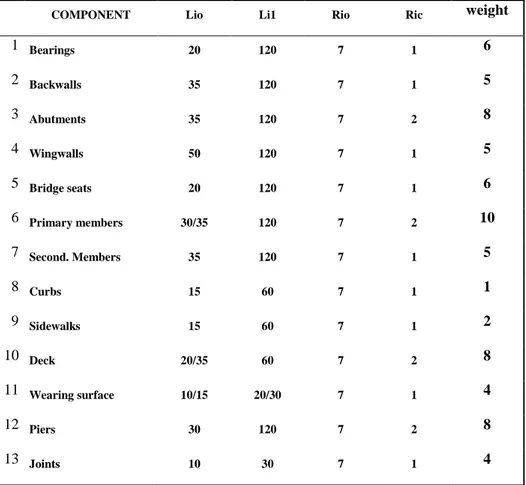
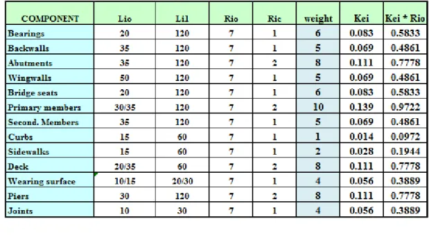
For every component is possible to assign, based on experience, an expected life that the component would have if the full maintenance was guaranteed every year (Li1) and an expected life due to a none maintenance (Li0). In the table 1 it’s possible to see for each component the importance weight, the shortest life, the longest life, the initial rating R (that means new component) and the Ric that is the rating that, if reached, means the failure of the component.

_COMPONENT _Lio _Li1 _Rio _Ric weight

1 _Bearings ₂₀ ₁₂₀ ₇ ₁ 6 2 _Backwalls ₃₅ ₁₂₀ ₇ ₁ 5 3 _Abutments ₃₅ ₁₂₀ ₇ ₂ 8 4 _Wingwalls ₅₀ ₁₂₀ ₇ ₁ 5 5 _{Bridge seats} ₂₀ ₁₂₀ ₇ ₁ 6 6 _{Primary members} _30/35 ₁₂₀ ₇ ₂ 10 7 _{Second. Members} ₃₅ ₁₂₀ ₇ ₁ 5 8 _Curbs ₁₅ ₆₀ ₇ ₁ 1 9 _Sidewalks ₁₅ ₆₀ ₇ ₁ 2 10 _Deck _20/35 ₆₀ ₇ ₂ 8 11 _{Wearing surface} _10/15 _20/30 ₇ ₁ 4 12 _Piers ₃₀ ₁₂₀ ₇ ₂ 8 13 _Joints ₁₀ ₃₀ ₇ ₁ 4

(12)

12

The rating of each component, Ri, decreases every year. The rate of deterioration of components (ri) is defined as:

And thus the rate of deterioration for the whole bridge is:

Once that the fastest rate of deterioration (ri0) and the slowest one (ri1) are found it’s possible to define the rate of deterioration as a function of the level of maintenance done on every component.

In the model proposed by (Testa & Yanev, 2002) in their article “Bridge Maintenance Level Assessment” it’s possible to choose among three kind of trend for the deterioration rate:

 Linear

 Exponential

 Secant

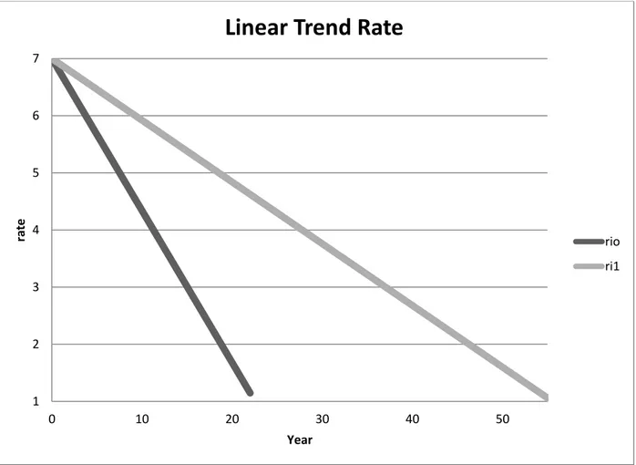
For example, by choosing the linear trend of rate deterioration, the ri0 and the ri1 are computed, for each component, by dividing the difference between the rate R “at new condition” and the critic rate by, respectively, the shortest expected life or the longest one.

( ) And ( )

(13)

13

In figure 3 it’s possible to see the linear rate for the two different rates ri1 and ri0. Naturally ri1 has a lower slope with respect to the rate with no maintenance and thus the critical rating for the given component is reached in more than the double time.

Figure 2 – Rate Linear Trend

Once understood this concept it’s easy to understand all the software working process. In fact, as it will be explained in next chapters, the expected life, the total annual cost as well as the overall Bridge Rating are function of the level of maintenance applied to the bridge.

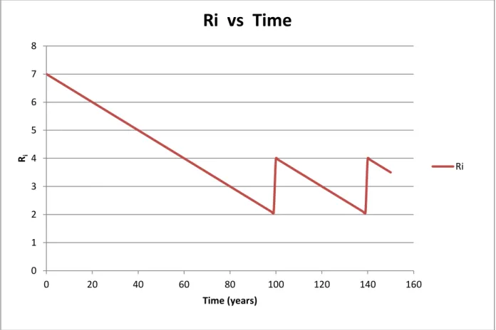
As it will be shown after, every time that the rateing of a component goes under a given threshold Rrep the component will be repaired and it will increase aging its Ri.

1 2 3 4 5 6 7 0 10 20 30 40 50 rate Year

Linear Trend Rate

rio ri1

(14)

14

Figure 3 - Trend of the Rating of a component in time

Maintenance

The maintenance is one of the most important points in this model under study. In fact almost the 20 % of the total expenditure of the New York City Department of Transportation is due to maintenance. Moreover, the maintenance, controls the deterioration rating of each of the 13 component thus is important to understand at all how it works. In this model the maintenance operations were divided into 15 main tasks:

 Debris Removal

 Seeping

 Clean Drainage

 Clean Abutment Piers

0 1 2 3 4 5 6 7 8 0 20 40 60 80 100 120 140 160 Ri Time (years)

Ri vs Time

Ri

(15)

15

 Clean Grating

 Clean Joints

 Wash Deck

 Paint (only for steel bridges)

 Spot Paint (only for steel bridges)

 Sidewalks & Curbs Repairs

 Pavement and Curb Seal

 Electric Maintenance

 Mechanical Maintenance

 Wearing Surface

 Wash Underside

Unfortunately it’s impossible, due to the actual budget condition, to assure a full maintenance for every component of every bridge. Hypothetically if a full maintenance was done on all the components of a bridge the expected life of it would be the longest possible. In this way less repairs or rehabilitations are needed and the decreasing drastically the costs for that. As it possible to see, in fact, for given component the rating, Ri, decreases fastest with no maintenance than with full maintenance (figure 4).

(16)

16

Figure 4 - Difference of R due to M

In the previous picture it’s possible to understand that, over a the same lifespan (in the example 70 years), the deterioration of one component with a full maintenance is slower than the one with none maintenance. In this example, during the 70 years the component with 100% maintenance will be repaired three times while, the component with 0% of maintenance, 9 times. As said in the paragraph (2.1), each repair, even if depending on the component, has an average cost of 25 million of dollars, this means that for the example on figure 4, New York City will spend 150 million of dollars more for the blue line with respect to the red one. Naturally, the annual cost of maintenance for the red line will be greater but the total annual cost at the end will be bigger for the “none” maintenance.

Why doesn’t New York City Department of Transportation do a full level of maintenance for whole the bridges if it’s cheaper than repair?

0 1 2 3 4 5 6 7 0 20 40 60 80 100 R ating R Time [year]

Rating Difference with different Level of Maintenance

R with 100% R with 0%

(17)

17

This approach could be doable if all the bridges were new (with a rating close to 7) and a perfect schedule of maintenance was programmed. Unfortunately the bridges system in New York City has an average age of 85 years old and until the 1970s no maintenance was done.

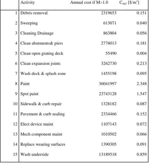
A previous study conducted at (Columbia University)1 in 1999 found which could be the total annual cost of a given task of maintenance done at what is thought to be 100% for the entire bridge system in New York and so, dividing the cost by the surface of the decks it possible to have an average of cost per square meter for every maintenance task (Table 2).

Activity Annual cost if M=1.0 Cmj1 [$/m 2

]

1 Debris removal 2319653 0.151

2 Sweeping 613071 0.040

3 Cleaning Drainage 863804 0.056

4 Clean abutments& piers 2776013 0.181

5 Clean open grating deck 55490 0.004

6 Clean expansion joints 3262730 0.213

7 Wash deck & splash zone 1455198 0.095

8 Paint 36041997 2.348

9 Spot paint 23743128 1.547

10 Sidewalk & curb repair 1328182 0.087

11 Pavement & curb sealing 2334466 0.152

12 Elect device maint 1107143 0.072

13 Mech component maint 1010502 0.066

14 Replace wearing surfaces 1390305 0.091

15 Wash underside 13189518 0.859

Table 2 Annual Maintenance Activities

1

(18)

18 Importance Factor Matrix

Fifteen maintenance activities were established and every bridge is divided into thirteen different components, it’s clear that not all the maintenance tasks have the same influence on the rate of deterioration of the bridge.

Therefore the model should keep in account how much a given task influences the overall deterioration of each component. To do that an Influence Factor Matrix was created. The Iij element of the matrix says how much the j-th task is important and useful for the j-th component. Every “I” factor is a number from zero to one. “0” means that i-th task is not important for that component while “1” means that is that is fundamental.

The Importance Factor Matrix (table 3) was established by a team of engineers in charge of maintenance and inspection section of the Department of Transportation. Albeit based on long experience, this matrix was assigned subjectively and thus it will be object of study in this work.

Components

Iij Brgs BkW Abut WgW Seats Prim Sec Curbs SW Deck Wear Piers Joints Debris rem 0.7 0.5 0.2 0.1 0.8 0.5 0.5 0.8 0.8 0.8 0.9 0.1 0.8 Sweeping 0.2 0.1 0.1 0 0.5 0.5 0.5 1 0.8 0.9 1 0.1 1 Clean Drain 0.9 0.9 0.9 0.8 1 1 1 1 1 1 1 0.5 1 T Clean abut/piers 1 1 1 0.9 1 0.8 0.8 0 0 0.5 0.5 1 0.5 a Clean grating 0 0 0 0 0 0 0 0 0 0 0 0 0 s Clean exp jts 1 0.8 1 0.5 1 1 0.8 0.5 0.5 0.9 0.9 0.9 1 k Wash deck etc 0.5 0.3 0.2 0 0.6 0.4 0.4 1 0 1 1 0.4 1

s Paint 1 0.5 0 0 0.5 1 1 0 0 0.4 0 1 0.5

Spot paint 1 0.5 0 0 0.5 1 1 0 0 0 0 1 0.5

Sidewalk & curb 0 0 0 0 0 0 0 1 1 0.1 0.1 0 0.5 Pavmt & curb seal 1 1 1 0.5 1 1 1 1 1 1 1 0.5 0.5 Elect device maint 0 0 0 0 0 0 0 0 0 0 0 0 0 Mech Comp 1 0.5 0.5 0.2 1 1 1 1 0 0.5 0 1 1

(19)

19

Repl wear surf 0 0.1 0 0 0.1 0.1 0.1 0.5 0.5 1 1 0.1 1 Wash underside 1 1 1 0.5 1 1 1 0 0 0.8 0 1 0.9

Table 3 Influence Factor Matrix

As it will be show in next chapters that value of the index matrix are used normalizing along the columns.

Repair, rehabilitation and user costs

In the model crated by (Testa & Yanev, 2002), as said before, repair, rehabilitation and user costs are taken into account. In fact, it’s normal that during the life span of a bridge, based on the level of maintenance that it is subjected, more or less number of repairs is necessary. While a standard repair of a component can be not very expensive and can last for few days or weeks, a partial or full rehabilitation of a bridge is very expensive (the cost for a full rehabilitation is estimated around 5,000 $ per square meter of deck) and can last from one to three years.

The user costs are additional costs introduced in order to take into account of traffic delays due to bridges closures and/or restriction for the circulation. These user costs were estimated by (Yanev & Testa) based on traffic data and economic indicators. A detailed explanation of how that user costs are introduced in the model will be given in the next chapter. It’s clear that user costs are strictly dependent on repair and rehabilitation costs.

The Model

As explained in paragraph 2.1 the model is based on the idea that changing the level of maintenance applied on a given components the velocity of deterioration of that component will

(20)

20

vary. By varying the ri the expected total life and the total annual cost change. The annual total cost is the summation of:

 Annual Maintenance

 Annualized Repair Costs over the entire life span of the bridge

 Replacement Costs over the entire life span of the bridge

 New York City Costs over the entire life span of the bridge

 User Costs over the entire life span of the bridge

In the model created by (Testa & Yanev, 2002) it’s possible to choose which trend to give to the rate of deterioration. It’s possible to choose between linear, exponential and secant trends. As already said the rate of deterioration is the speed with which every component tends to deteriorate over time.

For sake of simplicity all the work of this thesis will be done by using the linear rate of deterioration. Therefore the rate of deterioration will be defined as:

( ) ∑

Where:

 ri1 = deterioration rate if a full maintenance is done  ri0 = deterioration rate if no maintenance is performed

(21)

21

 ri = rate of deterioration for a given components following the linear trend

The software applied the deterioration rate to each component starting from an initial value (R = 7) to reach the need to a repair as soon as a component rating arrives at a designated level (Rri). At this point the components is repaired or replaced and the Ri is increased by some amount (dRi). All this values are chosen by the user. These components repairs are grouped at 5 years intervals. The critical components (primary member, piers, abutments and deck) can be repaired only two times in the whole bridge life and they are repaired at the 5 year mark preceding the time at which they reach Rri while the other components at the 5 year mark after.

The failure of the bridge occurs when at least one of the critical components reaches its R critical. Failure decides of course the life of the bridge.

The model takes also into account two different kinds of user costs: the first one considers the disruptions and the delay at each of the component repair events during the lifetime and the second is associated with the disruptions as a result from use the bridge when it has a low overall rating R. This second user cost is calculated as a percentage function of the bridge rating. For example, if the bridge has an overall R<4 the software adds a 20% of the estimated cost, if R<3.5 it adds a 50% if R<2 it adds a 100%.

(22)

(23)

23

Analysis of Existing Software

Key Components

Among the 13 components in which the bridge is subdivided there are 4 that are more important:

 Primary Member

 Piers

 Abutments

 Deck

All these components are essential for the right working of the bridge and so, if just one of that fails the entire bridge will fail. These components are then said “key components”. This is a true approximation, in fact, they are essential for the correct working of the bridge also in the reality. Without the deck or without the primary member the bridge can’t work.

Overview of the working of the software

In their work, (Testa & Yanev, 2002) created a software that can be used in order to compute, by varying the numbers of bridge, the level of maintenance, the bridge type and so on, the total annual cost that includes maintenance, repairs costs, NYC costs and user costs.

In this chapter the program working will be explained. The software is an excel files composed by 14 electronic spreadsheets:

 Task

(24)

24  Life  Matrix Iij  Costs  Calculation I  Calculation II  Chart Calculation

The first nine sheets are used to insert data and to do calculations while the last five are output graphs. A complete explanation of each sheet is provided below.

Task

The first sheet that appears opening the software is the “Task Sheet”. This spreadsheet is composed by two main tables: the Bridge System data and the optimization of for the maintenance frequencies and the relative annual costs.

The bridge system data (figure 5) permits to insert the number and the type of bridge that we want to analyze as well as the total number of spans and their area in square feet.

(25)

25

Figure 5 - NYC Bridges

As you can see it’s possible to distinguish between “pedestrian” and “non pedestrian” bridges.

(26)

26

Figure 6 - Activities Costs and Frequencies

In this first columns there are listed the different 15 kind of possible activities. In the second and third columns are shown the recommended frequencies of maintenance for each task if the 100% of maintenance would be possible. Kmi & Kmi*Mi columns will be explained in the “Matrix Kij” paragraph. Mi is the actual level of maintenance for which the analysis is computed. The “Annual Cost” columns has inside the hypothetical annual costs for each component and for the overall bridge system, controlled by The New York Time Department of Transportation, if the full maintenance (M=100%) would be possible. Cmli is the annual cost per square foot.

Components

This sheet is composed just by one table (fig 7) that has inside, for each bridge component, the following value:

(27)

27

Figure 7 - Components

 Li0 = expected life with no maintenance  Li1 = expected life with full maintenance  Ri0 = rating at start

 Ric = rating for component at failure  Weight = influence of component i

 Kei = normalized influence of component i on bridge rating on bridge rating

Life

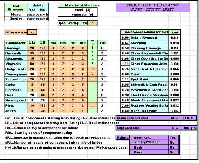
In the “Life” sheet the user can insert and choose the kind of data that he needs. This sheet is subdivided into three main parts. In the first one, bridge life calculation (figure 6), user has to choose the level of maintenance desired for each task with which make the analysis.

(28)

28

Figure 8 - Bridge Life Calculation - Input- Output Sheet

In this window the user is asked to choose the characteristics of the bridges that he wants to analyze. It’s possible to choose between:

 Steel/Concrete Bridges

 Mono/Overlag Deck Structure

 Open Grating or not

In the bottom-right part it’s possible to see the overall maintenance level of the bridge and the consequent expected life (in years).

(29)

29

Another important choice has to be done in this sheet: which kind of trend has to be used for the deterioration rate (figure 9). As said before, it possible to choose between linear, exponential and secant trend. Or sake of simplicity all the analyses, in this work, will be done using the linear one.

Figure 9 - Trend Input

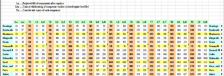
The last table that composes this sheet is the “Repair Schedule Aid sheet” (figure 10).

Figure 10 - Repair Schedule Aid Sheet

This calculation sheet is used, together with the Calculation I and Calculation II sheets to show the years in which in which the different components the selected repair rating Rri and so should be repaired.

(30)

30 Matrix Iij

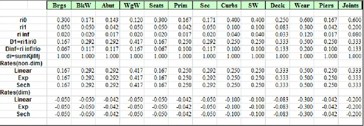
This is one of the most important sheets in the whole software. In fact it contains the Importance Factor Matrix Iij (figure 11). As explained before, thanks to this matrix, the program is able to “understand” how each activity of maintenance affects a given bridge component.

Figure 11 - Important Factor Matrix

All terms of this matrix were inserted deterministically thanks to the experience of the Department of Transportation engineers. As already said, this matrix will be the sujbet of study in next chapter. The colorful cells can change value by varying, in “Life” sheet, the bridge features from steel to concrete or from bridge with open gratings to bridge without them.

In this sheet every value Iij is normalized with respect to each columns co that in the Kij matrix (figure 12) the sum of the numbers in each column is equal to 1. By normalizing by column the effectiveness of each activity on a given task is highlighted.

(31)

31

Figure 12 - Kij Matrix

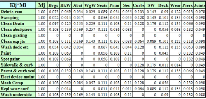
After that, a matrix that contains the multiplication of Kij by Mi is computed (Figure 13). This matrix is one of the key of the program, in fact, the deterioration rate for each component has is a function of the sum (on the column) of Kij * Mi.

Figure 13 - Kij*Mi

In the last part of the worksheet the matrix Kij*Kei and the value kmi are computed. These are then useful to calculate the life of overall maintenance level of the bridge and the expected life.

(32)

32 Calculation I and II

Calculation I and Calculation II are the two keys sheets of the program. Here, in fact, all the process of deterioration of the bridge components is developed. There are two windows where all the parameters useful for the calculation are computed (figure 14 and figure 15).

Figure 14 - Calculation of linear distribution

Figure 15 - Computation Parameters for Calculation

The core of the analysis is shown in (figure 14). Here the computed deterioration rate is used to decrease, year after year, the rating of each component. As soon as the rating Ri reach the threshold Rri it means that the component is not working as it should and then is repaired or replaced. The replacement brings up the rating of the component and so on. The keys components, primary member, Piers, Abutments and Deck can be replaced only twice in the entire life. After that the bridge reaches its expected life.

(33)

33

Figure 16 - Rate for each Components over the years

The last important table is the one that compute the number of time a component is replaced or repaired. This table (figure 15), computed thanks to “Calculation I” and “Calculation II” sheets will be used in “Costs” to compute the annualized expenditure due to repair and replacement.

(34)

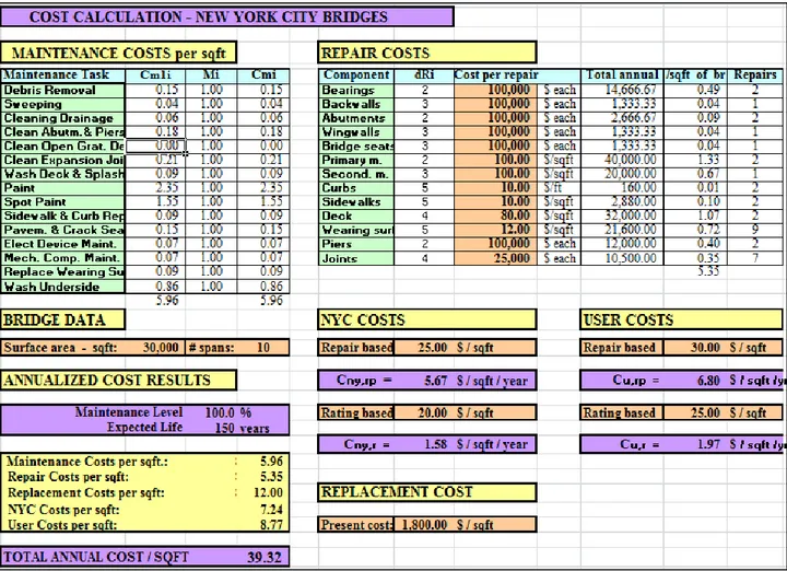
34 Costs

The last input/output data sheet is the “Costs” one (figure 18). In the upper part of this sheet, the user can insert the values of costs for the different kind of repairs associated with the different components. In the upper left part there is a table that report in summary three values for each maintenance activity: the actual level of maintenance performed, the cost per square foot if a full maintenance is done(Cmli) and the final cost per square foot at the given level of maintenance (Cmi).

Figure 18 - Costs Sheet

In the bottom part it’s possible to insert the bridge data for the bridge that we are analyzing and the repair, replacement and user costs.

(35)

35

In the bottom left part of the sheet there is a summary table reporting for our bridge, all the detailed cost of the sum of them: the Total Annual Cost per square foot.

Summary

In this sheet all the input data and the results of the analysis are reported (figure 19). In this simple table all the analysis information are reported. In fact all the unit costs for replacement and repairs are reported as well as the input bridge data or the detailed results with the total annualized cost.

(36)

36 Graphs

The others sheets contain graph like the annual cost per square foot subdivided in maintenance, repair and replacement cost, the unit maintenance cost VS the level of maintenance in percentage, the expected live VS the maintenance level and so on. It’s possible to have an idea about how this graphs looks like with the following pictures.

Figure 20 - Maintenence Level VS Annual Cost per square meter for uniform changes of Mi’s

0.00 100.00 200.00 300.00 400.00 500.00 600.00 700.00 800.00 900.00 00 10 20 30 40 50 60 70 80 90 100 Ann u al Cost ( $ / sq m / yr) pp Maintenance Level (%) Replacement Repair Maintenanc User Cit

(37)

37

Figure 21 - Expected Life VS Maintenance Level

Advantages of this Software

As all the programs this software presents some advantages and some disadvantages that we will highlight and try to correct by proposing some solutions. In the following paragraph all the advantages will be listed.

User friendly and speed

One of the biggest advantages of this software is the velocity with which it’s possible to running different scenarios (easily changing the parameters) and thus analyze different kind of bridge situations. Moreover, being an excel spreadsheet, it can be quickly understood by all kind of users. The interaction cell, in which the user can add or modify data are few and all easily identifiable having a colored fill.

00 20 40 60 80 100 120 140 160 00 10 20 30 40 50 60 70 80 90 100 E xpected L if e (y rs) Maintenance Level M (%)

Life of Bridge for Specified Repair and Maintenance Schedules

(38)

38 New York City Cost & User Cost

The program, as explained before, was thought in order to take into account the NYC cost and the User cost. These two kinds of costs were inserted to make the simulations more realistic. In fact they consider the discomfort due to a low bridge rating (R) as well as the time for the city department to make repairs or replacement of part of the bridges. Once the two costs are well calibrated based on people survey and detailed analyses they can become an important tool to run accurate simulations.

Broad range of parameter and components

The program permits to play around with a lot of parameters. Acting on 13 different bridge components and 15 possible tasks it has the possibility to launch an optimization analysis in order solve problems of annual budget allocation for New York City. In fact a limited maintenance budget resource should generally be allocated so as to maximize the overall maintenance level M. The level of maintenance M, takes into account subjective estimation of the Iij matrix coefficient and so, as we’ll see in the “disadvantage chapter”. It is also seen here, however, that there are differences in annualized cost among the various possible allocations at similar values of M.

Disadvantages and Problems of this Software

As all the software at their first version, also the bridge management software that we are analyzing has some questions to address. There are mainly three problems that should be correct. In the next paragraph, these three problems will be presented and in the next chapter a possible solutions will be presented.

(39)

39 Uniform level of maintenance

As we said in the past chapter, the user, when he/she is running an analysis, can choose which levels of maintenance performing for all the tasks. In fact, for every task the user can choose a level of maintenance that goes from 0% (no maintenance) to 100% (full maintenance or more). The full maintenance for every task is a utopia because it is almost impossible that the Department of Transportation had enough budgets to allocate in maintenance. It has also to be said that the M = 100% is the level of full maintenance evaluated by a group of specialist but it’s not the actual maximum level that could be done, as it will be shown in the last chapater. The chief engineer, by using also this kind of software, will have to decide how to best spend the budget by allocating the money in the task that better improve the total rating of the bridge.

The problem would rise if all the levels of maintenance are set at the same percentage. If this happened the Index Factor Matrix I would have no influence on the rate of deterioration ri and therefore no influence on the overall bridge rating. This problem can be easily explained mathematically. In fact, as it was illustrated in the chapter 2, the deterioration rate, for every component, goes as:

( ) ∑

Where:

(40)

40

 ri = rate of deterioration for a given components following the linear trend

The normalized index factors kij are normalized by the columns. This means that for every different component, the summation of the k is equal to 1. If there is an uniform maintenance level, therefore all the Mi are equal, and then the summation for all the task kijMij won’t be dependent anymore on the kij but it will just be function of the maintenance level.

For example, supposing that we are making a uniform level of maintenance M = 75 %, for the primary member the index factor are:

Iij Kij Kij*Mi Debris rem 0.50 0.05 0.04 Sweeping 0.50 0.05 0.04 Clean Drain 1.00 0.11 0.08 Clean abut/piers 0.80 0.09 0.06 Clean grating 0.00 0.00 0.00 Clean exp jts 1.00 0.11 0.08 Wash deck etc 0.40 0.04 0.03 Paint 1.00 0.11 0.08 Spot paint 1.00 0.11 0.08 Sidewalk & curb 0.00 0.00 0.00 Pavmt & curb seal 1.00 0.11 0.08 Elect device maint 0.00 0.00 0.00 Mech Comp 1.00 0.11 0.08 Repl wear surf 0.10 0.01 0.01 Wash underside 1.00 0.11 0.08 SUM Kij*Mi = 0.75

Table 4- Example Uniform Maintenance

As it’s possible to observe the level summation of Kij*Mi is equal to 75% that exactly the uniform level of maintenance done on the bridge. This means that, as explained before, the rate of deterioration is depends only on M and not on the Importance Factor Matrix. A possible solution for this problem will be addressed in the next chapter.

(41)

41 Few numbers of repair for the APPD components

The second question that will be addressed of this software is related with the method that it uses to determine the expected life of the bridge. As it was explained in chapter 2 the program runs the analysis until when the rating (Ri) of a primary component reaches the critical threshold Ric. The critical components are Abutments, Primary member, Piers and Deck (APPD). As soon as one of these critical ratings is reached, the component fails and with it the whole bridge. In order to avoid that a general component goes under its threshold value, as soon as the given component rating (Ri) reaches the rating of repair (Rri), another threshold decided by the user, the component is repaired.

The lack in stringency of the software is due to the fact the APPD components can be potentially repaired only 2 times in their life-span. The programmer had to impose this trick in order to make the analysis finish and not to go ahead to infinity. In fact, without this trick (table 5), every component, as soon as it reaches the Rri is repaired and the critical threshold Ric would never be reached.

Allowable Repairs and Relative Year

1st 2nd 3rd 4th 5th 6th 7th 8th 9th Bearings 70 95 125 150 180 205 235 260 290 Backwalls 75 125 170 215 260 310 355 400 445 Abutments 70 110 Wingwalls 85 130 180 230 280 330 380 430 480 Bridge seats 70 110 150 195 235 275 320 360 400 Primary memb. 70 105 Second. memb. 75 125 170 215 260 310 355 400 445 Curbs 35 70 105 140 175 210 245 280 315 Sidewalks 35 70 105 140 175 210 245 280 315 Deck 35 70 Wearing surf. 15 30 45 55 70 85 100 110 125 Piers 70 105 Joints 20 35 50 65 85 100 115 130 145

(42)

42

Even if this method permits to make the simulation ends given a reasonable expected life for the bridge, it is not engineering meaningful. In fact, as all the components of the bridges can be repaired all the times their Ri < Rri so should be allow to the APPD ones. It doesn’t make sense that they could be repair or replace only two times in the life of the bridge.

In order to make more accurate the program, deleting this end process but always staying in realistic range of life span, the entire “end-process” should be modify. An alternative solution and end process will be presented in the following chapter.

The component rating Ri is independent from the components weight

As explained in the previous paragraph, the program runs the analysis until when the component rating (Ri) of one among the Deck, Primary Member, Abutments or Piers reaches the critical rating (Ric).

It’s possible to perceive, by playing around with the software, that the component rating Ri is related in any way with the component normalized weight of the component with respect to the overall bridge components. This practically means that the importance a given component with respect to the other ones doesn’t influence the expected life of the bridge therefore the annual cost of maintenance. As previously said, it’s possible to assign at each component an importance factor from 1 to 10 (table 6). These factors, once normalized with respect to all the other ones, allow immediately to understand which are the most important components for the bridge correct behavior and which ones are not.

Component Weight Kei Bearings 6 0.083333 Backwalls 5 0.069444 Abutments 8 0.111111 Wingwalls 5 0.069444

(43)

43 Bridge seats 6 0.083333 Primary members 10 0.138889 Second. Members 5 0.069444 Curbs 1 0.013889 Sidewalks 2 0.027778 Deck 8 0.111111 Wearing surface 4 0.055556 Piers 8 0.111111 Joints 4 0.055556

Table 6 - Component Importance

In this table is highlighted in red the most important component that naturally is the primary member and the lowest one that are the sidewalks.

For a more accurate representation, the importance of the components should interact with the deterioration rate. A new approach to determine the failure of a components as well as the failure of the whole bridge will be presented in the next chapter.

(44)

44

Solutions for problems highlighted in chapter 3

In this chapter, plausible solution to the problems highlighted in the previous chapter will be investigated and presented. As we said there are three main problems that are the independence of the of the deterioration rate from the normalized importance factor and the strictly dependence on the uniform maintenance level, the fact that in not function of the importance of the bridge components and the max number of repairs to which the abutment, the primary member, the piers and the deck are subjected.

Significance of independence of M when uniform

As already said the maintenance problem occurs when every task is done at the same percentage of maintenance. This is very clear if we look at the formula that define the deterioration rate:

( ) ∑

Where:

 kijMi = summation of the products between the index factor Iand the maintenance level  ri = rate of deterioration for a given components following the linear trend

Thinking about this from a physical prospective it’s possible to realize that it is not really a problem. In fact this approach makes sense. If the level of maintenance is uniform it means that all

(45)

45

the tasks, from debris removal to wash underside are executed at the same level. If these are done with the same intensity it doesn’t matter how much one of this is important for a given bridge component with respect to the other because at the end of the day all the task, the less and the more important ones, will done at the same level.

In order to make the reader understand this concept, a small example is shown below.

The example is done by simplifying the software and by assuming that our system (bridge) has only two components and there are only three tasks doable on them. For sake of simplicity the two components are called “component 1” and “ component 2” while the tasks are “task 1”, “task 2” and “task 3”.

An Importance factor matrix for this simplify system is assumed (figure 22) as well as a realistic uniform level of maintenance for all the tasks (M = 80 %).

Iij Comp. 1 Comp. 2

Task A 0.5 0.3

Task B 1 0.5

Task C 0 0.1

Sum 1.5 0.9

Figure 22 - Importance Factor Matrix for example

By following the procedure illustrated by (Testa & Yanev) every Iij factor is normalized with respect to the column (every Iij factor is devided by the sum or the column) to have the Kij factor that are reported in (figure 23).

Kij Comp. 1 Comp. 2 Task A 0.33 0.33 Task B 0.67 0.56 Task C 0.00 0.11

(46)

46

And at the end, the last step is done: every Kij factor is multiplied by the level of maintenance established for the relative task (in this case M = 0.8) and the Kij*Mi values are found (figure 24).

Kij*Mi Mj Comp. 1 Comp. 2 Task A 0.80 0.27 0.27 Task B 0.80 0.53 0.44 Task C 0.80 0.00 0.09 sum KijMi 0.80 0.80 Figure 24 - Kij*Mi Matrix

Once the Kij*Mi matrix is done it’s possible to do the sum of this elements and, as it’s possible to see in the last row, are both equal. In fact, it’s possible to set whatever importance factor for a given element but if the level of maintenance is equal for all the task it doesn’t influence the deterioration rate.

All the maintenance task are done at a given level, for example M = 80%, and so every element will be effected by an equal maintenance, in this case 80%.

By summarizing, the importance factor matrix is a very important tool to analyze and model the behavior and the response of different maintenance tasks over a bridge.

(47)

47

Solution to the fact that k should be function of kei

As explained in the previous chapter, it’s strange that the both the deterioration rate and the bridge failure mode are not function at all of the relative importance of each bridge components, with respect to the other ones. If a component, for example the deck, is more important than another one, let’s say the curbs, it should be considered in the calculation.

This solution that will be presented here is only one among the possible ones. The conceptual change that will be illustrated is relative to the introduction of the Kei (the normalized weight of the bridge components) in the factor that decides the failure of the bridge.

The solution is a new failure test different from the previous one. By defining the following quantities:

∑

∑ ( )

∑

The failure will be governed by the following rule. There will be failure when:

MIN (A;B) < MAX (S;T)

Every critical rating components Rci is multiply for the relative normalized weight Kei. In this way the relative importance of each component with respect to the others, enters in the calculation. Then, as it was said before, there will be establish two new failure limits. The first is due to the sum of the Kei*Ric for all the components while the other is the sum of Kei*Ric for only the APPD components. This calculation is illustrated in the table 7.

(48)

48

Component Ric Weight Kei Kei * Ric Bearings 1 6 0.083 0.083 Backwalls 1 5 0.069 0.069 Abutments 2 8 0.111 0.222 Wingwalls 1 5 0.069 0.069 Bridge seats 1 6 0.083 0.083 Primary members 2 10 0.139 0.278 Second. Members 1 5 0.069 0.069 Curbs 1 1 0.014 0.014 Sidewalks 1 2 0.028 0.028 Deck 2 8 0.111 0.222 Wearing surface 1 4 0.056 0.056 Piers 2 8 0.111 0.222 Joints 1 4 0.056 0.056 SUMTOT 1.472 SUMAPDD 0.944

Table 7 - New Failure Test Index

These two numbers will be compared with deterioration rating at every year. And, in particular, the first one will be compared with the weighted average of the 13 component’s deterioration rates while the second value (SUMAPPD) will be compared with the weighted average of the four most important components: abutments, piers, primary member and deck. As soon as one of these two quantities reaches one of the two new threshold values, the bridge fails.

This new kind of verification permits to make more accurate analyses and to consider also, as an important parameter, the importance of a given component with respect to the others.

It has been possible to add the part that allows to verify the failure of the bridge and its relative expected life. Further implementation of the software will allow to find also other important values such as the consequent total annual cost of maintenance, replacement, repairs and add costs.

(49)

49

In order to give an idea about the changes that there are in the expected life, an example is proposed. A uniform level of maintenance is made increase from zero to 100% and the expected life is reported for both methods. In the figure 25 there are the two trends of this analysis.

Figure 25 - Expected Life for Old and New Methods

As it’s possible to see, for the most used level of maintenance (above the 60%) the new method of failure test gives a longer expected life. It will be implemented then.

Once that the software is updated with the annual cost it will be possible to evaluate if this new kind of failure test is better or not with respect to the old one.

0 20 40 60 80 100 120 140 160 180 0 20 40 60 80 100 120 Exp e cte d Li fe[y e ar s]

Uniform Maintenance Level

Comparison Expected Life Old and New Method

OLD NEW

(50)

50 Solution number of repair for APPD members

The limitation given by this problem is that the maximum expected life that is possible to reach using the software is 150 years. Is that a realistic value of expected life?

All around the world there are bridges that have a much higher life than 150 years, it’s possible to mention the Ponte Vecchio (figure 26) in Florence as well as the majority of the Venice bridges.

Figure 26 - Ponte Vecchio – Florence

Unfortunately that kind of bridges is different. The today bridges were and are built with other intents. They have to support huge loads given by multiple lines of car and trucks and sometimes also subway trains. They are subjected to great value of bending moment, torsion and axial force and especially they have to deal with fatigue due to dynamic loads. It’s easy to understand that they are subjected a more repairs and replacements during their life. However, the replacement operations, especially for primary components such as primary member, piers, abutments and

(51)

51

deck, are not easy at all. Moreover they can’t assure a completely new level of status. Every time that one of these APPD elements is replacement the bridge decreases the overall rating R.

Although it would be possible to modify the program in order to do not limit the number of repairs that is possible to do on the abutments, the primary member, the piers and the deck this operation is not suggested. In order to do that table 8 would have be modified increasing the number of repairs allowed.

Allowable Repairs and Relative Year

1st 2nd 3rd 4th 5th 6th 7th 8th 9th Bearings 70 95 125 150 180 205 235 260 290 Backwalls 75 125 170 215 260 310 355 400 445 Abutments 70 110 Wingwalls 85 130 180 230 280 330 380 430 480 Bridge seats 70 110 150 195 235 275 320 360 400 Primary memb. 70 105 Second. memb. 75 125 170 215 260 310 355 400 445 Curbs 35 70 105 140 175 210 245 280 315 Sidewalks 35 70 105 140 175 210 245 280 315 Deck 35 70 Wearing surf. 15 30 45 55 70 85 100 110 125 Piers 70 105 Joints 20 35 50 65 85 100 115 130 145

(52)

52

Analyses

In this chapter some results of relevant analyses ran with this software will be presented. In order to highlight the difference between the old standard software and the modified one the same analyses will be done using both the version of the software. In the first section will be shown the results due to the normal program while in the last section of this chapter will be presented the results from the modified program.

For both the kind of analyses the same bridge and the same unit cost will be used. Bridge sample and unit cost are presented in the following paragraphs.

Bridge sample for analyses

An analysis is different from another one based on the parameter that you put as variable data. Most important are the bridge data, that define the dimension, type, material and characteristic of the bridge and the cost data, that given the unit cost for repair, replacement and maintenance of components.

Input Bridge Data

In order to run analyses it needed to choose the kind and the dimension of the bridge to analyze. In order to make a realistic example, a standard bridge that can be found in New York City area is chosen. The characteristics of the bridge are list here:

 Bridge Area = 50 000 ft2 (equal to 2 790 m2)

 10 spans

 Material = Steel with joints

 Overlay Deck

(53)

53 Input Components and Repairs Costs

Every analysis has to account, as also said before, of costs of replacement and repair of single components or whole bridges. The unit costs are summarizing in the following list. All the values are an average of real money that the Department of Transportation of New York City usually spends to accomplish a given task. These unit costs were estimated in a study at Columbia University during 1999.

 Bearings 100 000 $ each

 Backwalls 100 000 $ each

 Abutments 100 000 $ each

 Wingwalls 100 000 $ each

 Bridge seats 100 000 $ each

 Primary member 100 $/ft2  Secondary member 100 $/ft2  Curbs 10 $/ft2  Sidewalks 10 $/ft2  Deck 80 $/ft2  Wearing Surface 12 $/ft2  Piers 100 000 $ each  Joints 25 000 $ each

(54)

54 New York Cost & User Cost

Among all the other data that have to be specified there are the New York Cost and the User Cost. As already explained they try to take into account the discomfort that a replacement or a repair makes to the city or to the citizens.

The two costs are here summarized:

 New York City Cost

o Repair Based: 25.00 $/ft2 o Rating Based: 20.00 $/ft2  User Cost o Repair Based: 30.00 $/ft2 o Rating Based: 25.00 $/ft2 Replacement Cost

The cost due to a replacement of a component is set as 1800 $/ft2.

Standard Software Analyses

In this section different kind of analyses, ran with the standard software, will be presented. The program is the one presented in the second chapter with the “problems” highlighted in the third chapter.

Utopian Full Maintenance

Here is presented the result due to a hypothetical analysis where a full maintenance of 100 % is done on the bridge. As we already said several time this level of maintenance is impossible to be reached in New York City due to its cost. This would have been possible if the full maintenance had

(55)

55

done, on every bridge, from when they were built. Unfortunately there was a long period in which engineers didn’t think a regular maintenance was so important for the life of the bridge and they preferred to repair or replace a piece when it failed to prevent that it did.

A full maintenance, when done correctly, is the one that brings to the longer expected life (in this software fixed in 150 years) and in the lowest total annual cost (based on the value estimated by the specialist and not based on the software optimizations). This value, that is the sum of annualized repair, replacement, user, New York City cost plus the annual maintenance cost figure 26), is much lower to respect a “realistic maintenance” one to do the small replacement cost.

Figure 27 - Annualized Costs Table

maintenance-level for task Kmi 1.00 Debris Removal 0.110

1.00 Sweeping 0.045

1.00 Cleaning Drainage 0.105 1.00 Clean Abutments& Piers 0.095 1.00 Clean Open Grating Deck 0.084 1.00 Clean Expansion Joints 0.100 1.00 Wash Deck & Splash Zone 0.050

1.00 Paint 0.054

1.00 Spot Paint 0.050

1.00 Sidewalk & Curb Repair 0.010 1.00 Pavement & Crack Sealing 0.100 1.00 Elect Device Maintenance 0.000 1.00 Mech. Component Maint. 0.075

(56)

56

1.00 Replace Wearing Surfaces 0.030 1.00 Wash Underside 0.093

Figure 28 - Maintenance at 100%

Standard Maintenance

The following result can be considered as a reference for all the analyses that will be shown. This is a realistic level of maintenance that can be done on a bridge in New York City. As then reported in (table 10) the overall level of maintenance is 78.6 % (a 72% of the hypothetical full maintenance cost) and the consequent expected life is equal to 104 years.

Figure 29 - Standard Maintenance Level

(57)

57

Table 9 - Costs of Standard Analysis

Comparison between Full Maintenance and Standard One

In this small section the differences between realistic values of maintenance analysis and the full maintenance one are highlighted. In the table 11 the expected life as well as the different annualized costs are reported for the full and for a 78% level of maintenance.

FULL REALISTIC Differences

Maintenance Level [%] 100 78.62 21.38 %

Expected Life [year] 150 104 46 Years

$/ft2/yr $/ft2/yr

Maintenance Costs 5.96 4.29 1.67 $/ft2/yr

Repair Costs 4.72 7.07 -2.35 $/ft2/yr

Replacement Costs 12.00 17.37 -5.37 $/ft2/yr

NYC Costs 7.24 9.46 -2.22 $/ft2/yr

User Costs 8.77 11.43 -2.66 $/ft2/yr

TOTAL ANNUAL COST 38.69 49.62 -10.92 $/ft2/yr

Table 10 - Cost Differences Full/Realistic Maintenance

From figure 30 is possible to appreciate the cost differences between the two methods. The full maintenance allows to reach an expected life 46 years longer than the realistic one.

Speaking about annual cost, it’s possible to see that the only one in which the full is bigger than the realistic is the maintenance cost. This is reasonable in fact the level of maintenance, as

(58)

58

therefore the time and the work to reach it, are grater. For what concern all the other annual cost, the full maintenance would be much cheaper than whatever realistic one. As it’s possible to see from the total values the full maintenance would be 22% cheaper than the realistic one.

Figure 30 - Full VS Realistic Maintenance Cost

In a bridge like the one that is analyzing that mean an annual saving of money of about 540’000 dollars. Unfortunately, as said, the full maintenance for all bridge is undoable and thus all the further analysis will be done using the “realistic” level of annual maintenance as a reference value.

1° Simulation: Step Maintenance increase for each element separately

The first simulation consists in increasing one maintenance level at time from 0% to 90%. In this way is possible to see, based on the level of maintenance, which is the total annual cost trend for each tasks. The main purpose of this analysis is to show that even if the total annual unit cost is an important parameter the expected life is much more significant. The trend of the expected life (figure 31) and the unit annual cost (figure 32) is shown in the following pictures.

0.00 5.00 10.00 15.00 20.00 25.00 30.00 35.00 40.00 45.00 50.00 A n n u al Un it Co st [$/ ft 2/y r] Full Maintenance

(59)

59

Figure 31 - Life VS Maintenance Trend

It’ clear, as it could be imagined that the more maintenance is done the longer is the expected life of the bridge. By the way, there is some difference in the maintenance level VS Life from task to task. While some tasks has a perfectly linear behavior (for example Paint, Mech. Components..) other ones has a non -linear behavior increasing relevantly the expected life when they are done over the 60%. 96 98 100 102 104 106 108 110 112 114 116 0% 20% 40% 60% 80% 100% Exp e cte d Li fe [Year s]

Life VS Maintenance

Standard

Debris Sweeping

Cleaning Drainage Clean Abutments& Piers

Clean Open Grating Deck

Clean Expansion Joints

Wash Deck & Splash Zone Paint Spot Paint Sidewalk Repair Pavement Electric Devices Mech. Components Replace Wearing Surface Wash Underside

(60)

(61)

61

Figure 32 - Unit Cost VS Level of Maintenance

44 45 46 47 48 49 50 51 52 53 0% 10% 20% 30% 40% 50% 60% 70% 80% 90% 100% Unit Co st [$/ ft 2]

Mainentance Task Cost VS Level of Maintenance

Debris Sweeping Test Cleaning

Cleaning Open Grating Clean Open Grating Deck

Wash Deck & Splash Zone Clean Joints Wash Deck Paint Spot Paint Sedewalk Pavement Electric Devices Replace Wearing Surface Wash Underside

(62)

62

As it’s possible to see in figure 31 there is some task that will give a lower cost when is not done. This means that for an economical point of view it could be better to do not make that task with respect to do it at a high level. One of these examples can be “Clean opening Grating”. On the other hand, there is some task that is better to be performed at a high annual level (above the 65%). One of these can be “Clean Joints”. All the costs above are the total ones that keep into account all the five cost and not only the maintenance one and thus there is not a linear behavior that it could be imagined. In fact the total costs are function of the numbers of replaces, repairs and discomfort due to that works.

Simulation 2. Keeping only Index Factor Iij bigger than 0.5

This simulation is done base on the Importance factor matrix. The purpose of this analysis is to see if doing a most effective maintenance is better than do a standard one. If fact, each element of the importance factor matrix in figure 33, means how important is the task for a given component with respect to the other components. For example, the element I16 = 0.8 of the following matrix means that clean the abutments and the piers is very important end effective for the primary members deterioration rate and so for its expected life.

In this analysis the standard Importance factor matrix (figure 33) is modified. For the most important components (Abutments, Primary Member, Piers and Deck) all the importance factor of the matrix, smaller than 0.5, are deleted.

(63)

63

Figure 33 - Standard Importance Factor Matrix

Putting a zero as the importance factor means that that task is not made on that components and thus it is done better one the other components. Being the APPD components the most important ones, the ones that bring to failure the bridge, we want to look how the expected life and the total cost behave by doing the maintenance only where it is more effective.

The modified importance factor matrix that is used for this analysis is the one represented in figure 34.