This paper aims to address the effects produced by the participation of farms in a set of schemes of the EU rural development policy (RDP) – known as pillar 2 of the Common Agricultural Policy (CAP) – that are intended to help meet the aims of the Lisbon strategy, i.e., higher economic growth, job creation and greater competitiveness in the world market. This set of measures (hereafter, growth-oriented measures – GOMs) mainly provide support for in-vestment in agricultural holdings and the establish-ment of young farmers. They cover only one-third of the total rural development policy contributions but play an important role, especially in the southern regions of the EU, because they have long been the only source of public support for farms specialising in the production of Mediterranean crops, which are not eligible for direct support payments delivered under pillar 1 of the CAP. More generally, GOMs are intended to address the limited access of farmers to credit (Benjamin and Phimister 2002; Blancard et al. 2006), and to help them incorporate those new technologies that promote survival, efficiency and growth in a competitive industry. In this way, GOMs
contribute to the economic growth of the sector and that of the entire economy. However, empirical evi-dence has shown that capital subsidies may result in over-investment, inefficiency in capital use, biased allocation of resources1 and windfall gains when subsidies are claimed by farms that would have made the investment anyway. Investment can also produce a loss of know-how and established routines, for ex-ample, the replacement of old machinery with new equipment. Consequently, we assess the net impact of GOMs on farm performance-related variables.
To determine whether significant and causal differ-ences in the outcome variables are evident between farms that receive a subsidy and those that do not, we explicitly consider the possibility of selection bias due to non-randomised programme participation and utilise a conditional difference-in-differences approach (Heckman et al. 1998). The selection bias problem occurs because we seek to determine the effect of a treatment (in our case, the effect of participation in an RDP measure) on outcomes on participating farms; however, we cannot observe the outcomes with and without treatment on the same individual
Rural development policy in Italy: the impact of
growth-oriented measures on farm outcomes
Cristina SALVIONI*, Dario SCIULLI
Department of Economic Studies, University of Chieti-Pescara, Pescara, Italy
*Corresponding author: [email protected]
Salvioni C., Sciulli D. (2018): Rural development policy in Italy: the impact of growth-oriented measures on farm
out-comes. Agric. Econ. – Czech, 64: 115–130.
Abstract: Growth-oriented measures of the EU’s rural development policy have been promoted to meet the aims of the
Lisbon strategy. Th is article assesses their impact on performancrelated variables of farms. We apply a conditional diff e-rence-in-diff erences approach to the 2003–2007 Italian FADN survey. No evidence emerges to indicate any impact of the measures on farm income, employment or partial productivities. Conversely, participation in the selected policy schemes resulted initially in a productivity increase and, subsequently, in enhanced farm performance. We argue that participation in the growth-oriented measures gave rise to a process of capital deepening that, in turn, elicited a productivity increase and, eventually, positive growth rates in farm performance. Th e estimated variations in capital intensity signal that the mea-sures resulted in the activation of channels that are expected to positively aff ect farm performance after a time lag.
Keywords: CAP, farm support, rural development policy, treatment eff ect
1For instance, capital aid provided by the ‘Green Plans’ in Italy during the 1960s resulted in over-investment in
farm at the same time. Simply comparing the mean outcomes may not reveal the actual treatment effect because participants and non-participants typically differ, even in the absence of treatment (Caliendo and Kopeining 2008). For example, it has been shown that in Italy small farms are more likely to participate in RDP (Pascucci et al. 2013). Failure to account for treatment selection bias can lead to a biased estima-tion of the true treatment effect.
The number of empirical studies that have examined the impact of agricultural and rural policy measures and that have controlled for the non-random as-signment of subjects to treatment is rapidly grow-ing (Esposti and Sotte 2013); however, so far, only a few address the RDP of the CAP. More specifically, the first applications evaluate the impact of agri-environment measures (AEMs) (Pufahl and Weiss, 2009), while more recent studies focus on investment support measures. Kirchweger et al. (2015) assessed the impact of an agricultural investment support programme in Austria on the income of dairy farms. They found that farm income increased significantly more on participating farms than on control farms. Ortner (2012) also studied the impact of investment support provided to Austrian farms, and found a positive effect on Gross Value Added. Medonos et al. (2012) showed that participation in a measure granting support to investments aimed at modernis-ing Czech farms significantly increased Gross Value Added and labour productivity. They also suggested, on the basis of the results of a qualitative analysis, the existence of significant deadweight losses. The issue of complementary or substitution effects of investment support under the RDP was explicitly investigated by Michalek et al. (2012). Using a sample of German dairy farms, they found a 100% deadweight loss; i.e., on all the farms, investment would also have been undertaken without the support. Chabé-Ferret and Subervie (2013) estimated additional and windfall effects of five AEMs for a sample of individual French farmers. Their findings show that subsidising the planting of cover crops is not cost-effective. In con-trast, the subsidisation of grass buffer strips could be socially efficient despite large windfall effects. They finally estimated that subsidising the conversion to organic farming has low windfall effects and high ad-ditionality. Udagawa et al. (2014) applied propensity score matching and difference-in-differences analysis to estimate the impact of farmer participation in an agri-environment scheme on cereal farm incomes in eastern England. The results indicate firstly that entry
into the programme has a negative impact on the total farm business income, which decreases over time; secondly, that losses are channelled mainly through the utilisation of land resources rather than through increased use of labour; and finally, that payments do not overcompensate for income losses.
Our paper aims to contribute to the scarce lit-erature on the evaluation of the RDP. We evaluate the impact of the GOMs implemented during the first programming period (2000–2006) of the Italian RDP on economic results and productivity on Italian farms. In fact, the literature that investigates the link between investment and firm productivity, starting with the seminal paper of Power (1998), predicts that there is often a lag phase between the point at which the investment is carried out and its effect on farm performance. This is because investment may require a learning period and/or the reorganisation of some production units, both of which are costly in the short term, and explaining why the effect of investment on firm performance is usually found to be negative in the short run. In consideration of this, in this paper, we assess the impact of participation in GOMs both on a set of performance-related vari-ables (gross output, employment, farm income and partial productivities), as well as on a set of indica-tors of capital accumulation (land and machinery capital stock, capital-land and capital-labour ratios). The variables in this latter set can be interpreted as precursors of growth, because changes in their levels signal the activation of channels through which in-vestment eventually impacts productivity and other farm performance-related variables in the long term. With the aim of assessing the impact of GOMs on farm performance, we use data from the 2003–2007 FADN sample, which allows us to assess the impact of the 2004–2006 GOMs on a number of farm outcomes observed in the year 2007. On the one hand, such an approach allows us to first evaluate whether the core mechanisms behind growth have been activated. On the other hand, however, because a longer time span is required in order to determine the effects of GOMs on farm outcomes, this analysis cannot fully represent growth effects.
The empirical approach consists of a conditional difference-in-differences method. In this respect, because farms can simultaneously benefit from dif-ferent CAP measures, the identification of the causal effect of a specific measure requires that the treated and the control groups be correctly selected to avoid spurious results. For example, direct payments
de-livered under CAP pillar 1 are expected to favour the allocative efficiency of farms (Moro and Sckokai 2011) and hence to reinforce the impact of the GOMs. In contrast, AEMs can represent a constraint on the rapid adjustment towards more efficient output; con-sequently, they can offset the impact of the GOMs. We disentangle this problem by basing our analysis firstly on “pure” comparison and treatment groups, i.e., comparing farms not benefitting from any pay-ment from the CAP to farms receiving paypay-ments from GOMs only, and secondly, by comparing the performance of farms receiving both pillar 1 and GOM benefits (treated farms) to that of farms receiv-ing only pillar 1 payments. This strategy allows us to compare the impact recorded on farms specialising in Mediterranean crops, which were excluded from the benefits of pillar 1, to that of farms specialising in the production of more continental products typi-cally targeted by pillar 1 support.
BACKGROUND
The EU’s RDP evolved from a policy addressing structural problems of the farm sector into an in-tegrated rural development policy, which no longer addresses one specific sector, i.e., agriculture, but rather a territorial entity, i.e., rural areas. Agenda 2000 established RDP as the second pillar2 of the EU’s CAP and brought rural development under a single regula-tion that applies across the whole of the EU for the 2000–2006 period. In 2005, the RDP was restructured into three thematic axes for the 2007–2013 period3: (i) improving the competitiveness of the agricultural and forestry sector, (ii) improving the environment and the countryside, and (iii) improving the quality of life in rural areas and encouraging the diversifica-tion of the rural economy.
O verall, the RDP aimed to contribute to the Gothenburg and Lisbon Strategy goals, that is, to improve the ecological sustainability of develop-ment, encourage economic growth and job creation in rural areas and increase the competitiveness of EU agriculture on world markets. The ecological sustainability issue was mainly addressed through a set of agro-environment measures falling under axis II. They were the only compulsory measures and
cov-ered 45% of total expenditure in the first programme period. The Lisbon Strategy was mainly represented by a set of measures that targeted farm restructur-ing and competitiveness (axis I) and another group of measures that aimed to improve the quality of life in rural areas and encourage the diversification of economic activity (axis III). The increase in farm income and profitability and the enhancement of the quality of life of the rural population induced by support provided by these two groups of measures were intended to revitalise rural areas and slow the ongoing process of land abandonment and rural depopulation.
To implement the RDP, each of the Italian regions and autonomous provinces prepared a programme with a total budget of EUR 14 million over the 2000– 2006 period. The financial resources of the 21 different Italian RD Programmes were mainly concentrated on measures directed at preserving and, where possible, enhancing the environment. In contrast, the policy measures devoted to promoting non-agricultural rural development, such as the diversification into non-farming activities and rural infrastructure devel-opment, approximately covered only the mandatory 10% of total spending. Finally, measures aimed at enhancing agricultural restructuring and competi-tiveness (GOMs) covered approximately one-third of the total contributions. Specifically, these meas-ures represent investments in agricultural holdings (12.6%), the establishment of young farmers (5.8%) and improvement in the processing and marketing of farm products (6.5%).
Overall, this latter group of measures were aimed at increasing efficiency in farming and enhancing the quality of agricultural production by promoting farm restructuring and modernisation. Specifically, the support offered for investment in agricultural holdings was aimed at eventually increasing the value added of the farm sector by reducing production costs, increasing sales and margins through better product quality and process control or promoting the diversification of farm resources in off-farm activities more profitable than farming. Similarly, the support for investments improving processing and marketing of farm products was aimed at increasing the value added, for example, by improving or rationalising marketing channels or improving the presentation
2Pillar 1 consists of direct area- and livestock-related payments available to nearly all farmers, export subsidies, support
for intervention buying and storage and a few independent market regimes.
and preparation of products, encouraging better use or elimination of by-products or waste or applying new technologies. Finally, the aim of the support for the entry of young persons into the agricultural sector was two-fold. It was intended partly to curb the ongoing depopulation of rural areas and partly to attract more young farmers, who are usually more productive, have a more positive attitude towards risk and are more open to change than older farmers. Additionally, the increase in farm income generated by these measures is expected to make farming a more attractive business. Ultimately, GOMs share the common goal of increasing the farm sector income and employment; consequently, they are intended to eventually contribute to the economic growth and job creation goals enshrined in the Lisbon Strategy.
METHODS AND DATA Theoretical background
The decision to participate in GOMs can be con-textualised in a farm household model, in which a household makes two sequential decisions – whether to participate and how much to invest – aimed at maximising the farm’s household utility. As suggested by Chabé-Ferret and Subervie (2013), the maximisa-tion problem can be solved by backward inducmaximisa-tion.
Investment decision and capital subsidies
Investment is defined as an increase in capital stock, and it should lead farms to the optimal capital stock, which represents the core of the investment behaviour problem. Economic theory, explicitly or implicitly, assumes a link between investment, productivity and economic growth4.
According to the neoclassical model of capital accumulation, the optimal level of capital stock is pursued by investing up to the point where the value of the marginal product of capital is equal to the user’s cost of capital. Firms often have less than the optimal capital stock due to the presence of capital constraints, adjustment costs and capital market imperfections; additionally, farmers are often risk-averse (Rosenzweig and Binswanger, 1993). Capital subsidisation can relax these constraints and increase
farmers’ willingness to invest in productive assets that increase farm profitability. The capital subsidies reduce the user’s cost of capital and increase the propensity to invest. The reduction in the user’s cost of capital is expected to induce a cost-minimising firm to substitute capital for labour and thus become more capital-intensive.
The decision to enter the support scheme
The farm household decides whether to enter a GOM scheme based on the net expected utility gain of the application costs5 associated with enrolment in the measure. Because the benefits and costs of participating differ among farms due to observable and unobservable characteristics, the estimated causal effect that is determined by comparing the outcomes of participants and non-participants is likely to be affected by selection bias. This bias results in an overestimation of the causal effect of the policy meas-ure because even without subsidies the participants would have had higher investment on average than the non-participants. In the context of GOMs, the self-selected farms are likely to be those that expected to have higher returns on their investments due to, for example, a favourable socio-economic environ-ment, higher factor endowenviron-ment, lower risk aversion or lower application costs.
Estimation method
When estimating the causal effect of participation in the GOMs on the outcomes of Italian farms, we operate in a non-experimental setting, for which the estimation of the causal effect of the treatment variable relies on the construction of a counterfactual using the observational data of untreated farms.
In the presence of non-randomised experiments, the most common parameter of interest is the so-called average treatment effect on the treated (ATT), which evaluates the average impact received for the subset of farms that have actually benefitted from GOMs against the farms that have not benefitted from them. However, as suggested by the theoreti-cal background above, we interpret participation in GOMs as a voluntary decision that aims to maximise the farm’s household utility. This choice is reasonably guided by the anticipated gains from participating
4However, there is still limited empirical evidence of such a connection.
5Application costs refer to the money and time spent preparing the application, which can vary depending on the
or not participating in the programme. Hence, the probability of participation diverges across the farms according to the observable and unobservable factors that determine self-selection for the programme. When a selection bias problem arises, it should be addressed using specific techniques when construct-ing the counterfactual.
One possible way to estimate the ATT consists of using cross-sectional matching estimators (Caliendo and Kopeinig 2008), for which each participant unit is paired with an observably similar non-participant and the difference in their outcomes (Y1 and Y0) is interpreted as the causal effect of the measure. However, this procedure does require identifying some assumptions. The first assumption seeks to address the selection bias problem by requiring that the outcomes be independent of programme par-ticipation (D) conditional on a set of observable characteristics (Z). This assumption is also called a conditional independence assumption (CIA). In this context, Rosenbaum and Rubin (1983) suggested that when Y0 is independent of programme participation conditional on Z, it is also independent of the prob-ability of participation p(Z) = Pr (D = 1|Z), where D is a binary variable indicating whether the farm has been treated.
Additionally, because matching is only justified if performed over the common support region6 (Heckman et al. 1997), our estimations are based on observations of the treated farms whose p-scores are higher than the minimum or lower than the maximum
p-score of the untreated farms. Moreover, to ensure
that the densities are strictly greater than zero, we require that they be strictly positive and exceed zero by a threshold amount determined by a “trimming level” q (see Smith and Todd 2005)7.
Cross-sectional matching estimates assume that the observed characteristics describe all of the systematic differences between the programme participants and the non-participants. However, the possibility of
pro-gramme selectivity based on unobservable factors or because of level differences in the groups’ outcomes cannot be discarded. With the aim of resolving these shortcomings, we exploit the longitudinal dimension of our dataset and adopt a difference-in-differences matching approach (or conditional difference-in-differences, CDID), as proposed by Heckman et al. (1997). The CDID estimator identifies treatment effects by comparing the change in outcomes for the treated farms to the change in outcomes for the control farms. Notably, the CDID estimator allows incorporation into the programme to be based on both observed and unobserved time-invariant farm characteristics. The CDID estimator requires that:
| ( ), 1
| ( ), 0
0 1 0 1 0 0 0 0 Y p Z D EY Y p Z D Y E t t t t (1)where t1 represents a time period after the treatment start date and t0 represents a time period before the treatment. Therefore, it follows that CDID compares the conditional before and after outcomes8 of the treated with those of the untreated:
| ( ), 1
| ( ), 0
0 1 0 1 0 0 0 1 Y p Z D EY Y p Z D Y E t t t t (2)The identification strategy of the CDID estimator, aside from the CIA, requires two further assumptions. The first is the stable unit treatment value assumption (SUTVA), which assumes that the treatment does not produce spillover effects on untreated farms; i.e., the treatment effects on non-participants is null9. The second is the conditional independence of increments assumption (CIIA), in which the average increment in outcomes before the treatment is equal between the participants and the control non-participants10. A varied set of matching estimators have been pro-vided by the literature. We use two different matching estimators to evaluate the impact of GOMs. The first is local linear regression (LLR) matching, and the second is the nearest-neighbour matching (NNM) estimator. The LLR estimator is a generalisation of the
6The common support region is that for which the support of the covariates overlaps for both the treatment and control
groups.
7We have set the trimming level to 1%.
8Dehejia and Wahba (2002) argued that estimation bias in matching methods can be reduced by using simple
pro-pensity score matching and controlling for past outcomes. In contrast, Heckman and Navarro-Lozano (2004) reject this hypothesis, while Smith and Todd (2005) argue that the Dehejia and Wahba’s (2002) result is due to the special structure of their dataset. As a further robustness check, we also ran simple matching to control for past outcomes. Related results are available upon request.
9In our context, SUTVA could hold if farms are price-takers and there is a low take-up rate. It follows that the subsidised
farms are likely not to affect the market, avoiding any transmission effects on the non-participant farms.
non-parametrical kernel matching method, for which each participant is paired with a weighted average over multiple farms in the comparison group. The LLR estimator performs better than kernel matching due to a faster rate of convergence near boundary points and greater robustness with different data design densities. According to the NNM estimator, each par-ticipant is paired with the closest non-parpar-ticipant(s) depending on a propensity score. In other words, a neighbourhood is defined for each participant (see Todd 2008 for a deeper analysis).
Data and definition of variables
The following analysis is based on a dataset that was constructed using information collected yearly by the Italian Farm Accountancy Data Network survey (FADN). This survey is conducted on a statistically representative random sample that has drawn from the census since 2003. The field of observation is the total number of commercial farms, that is, farms with an economic size greater than 4 ESU (EUR 4800). Commercial farms are the most important portion of the farm population when assessing the impact of RDP measures because minimum eligibility thresholds are often introduced to exclude small farms. From the FADN sample, we extract a five-wave balanced panel of 6542 farms containing only those holdings for which information was collected in all the years from 2003 to 2007.
The FADN gathers information about payment amounts that are received annually by farmers under pillar I. As for the RDP support, the survey records information about payments received by farmers participating in agri-environment schemes and in the following GOMs: investment in agricultural hold-ings (land improvement, purchase of machinery and equipment, etc.), investment in the processing and marketing of agricultural products, afforestation of agricultural land, implementing demanding standards, the establishment of subsidies for young farmers and vocational training. At the EU-25 level, the FADN covers up to 92% of the total RDP expenditure, with an average 35% participation rate (23% receive LFA payments, 18% agro-environment payments and 6% investment subsidies) (EC 2009). Among the Member
States, Italy has (together with Spain) the lowest proportion of RD recipients (17%). The panel data used in our study well reflect this situation.
Farms often benefit differently from pillar 1 and pillar 2 measures. When we estimate the causal effect of a treatment on outcomes, the overlap of measures makes it difficult to identify the impact of a specific measure, and this difficulty could possibly lead to spurious results. To disentangle the problems due to the interaction between simultaneous interven-tions that can affect farm choices and farm output, our identification strategy consists of defining the treatment group as the farms that received only GOMs and our control group as the farms that did not receive any CAP payment. Therefore, farms that have simultaneously received GOMs and other CAP benefits are excluded from the analysis. Additionally, given the available data and the model requirements, those farms that did receive benefits from the GOMs in 2003, that is, in the year used as the pre-treatment period, are excluded from the sample. The 2007 wave information is used to define our outcomes. Finally, the 2004–2006 waves are used to identify the treated (28) and the non-treated farms (1043). In this regard, it is important to recall that the one-year post-intervention period considered in this study might be too short to measure the total effect of the GOMs, or other structural policy measures, on farm performance-related outcomes. The choice of such a short post-intervention period is due partly to the unavailability of a longer span at the time the analysis was performed and partly to the fact that due to the sample turnover, the sample size declines steeply as the time span increases. In other words, even if new and more recent waves of data have become avail-able, the chances of following a farm participating in GOMs over a long enough period of time to make inferences about their causal impact do not improve.11 Although the period under analysis is probably too short to assess the total effect that the participation in GOMs is going to produce in the long term on farm performance, we can still check whether the capital intensity increases, signalling the activation of channels through which investments eventually impact productivity and other farm performance-related variables in the long term.
11In the FADN, panel data is currently available by accident rather than by design, and this limits its utility, especially
in the case of impact assessment of GOMs as well as other long-term policies. An explicit longitudinal panel, within the overall sample and suitably weighted, would increase the value of FADN as a research tool, because it would al-low better evaluation of many important policy issues and analysis of dynamic phenomena such as structural change.
It is worth noting that, due to the exclusion of farms receiving pillar 1 payments, neither group contains any farms specialised in the production of arable crops or olives and neither has more than a low percentage of farms specialised in livestock. The most common types of farming are specialised in horticulture, vineyards and fruit. The high per-centages associated with these types of farming well reflect the features of Mediterranean agriculture. In conclusion, the exclusion of farms receiving pillar 1 payments has the negative effect of reducing the size of the sample under analysis, although it has the great advantage of allowing us to focus on farms specialis-ing in the production of Mediterranean crops that are not eligible for pillar 1 and that hence use RDP measures as their only source of public support.
Because a relevant proportion of farms apply for and receive pillar 1 payments, the identification strategy based on the exclusion of farms receiving payments other than GOMs results in a large loss of observa-tions. Consequently, we replicate our investigation on a sample of farms receiving payments from both pillar 1 and GOMs (41), while the control group is composed of farms receiving only pillar 1 benefits (2150). It is worth noting that the inclusion of farms benefitting from pillar 1 is associated with larger per-centages of farms specialising in arable crops (eligible for pillar 1 support) and smaller percentages of farms specialising in the production of horticultural crops, fruit and wine (not eligible).
Definition of the treatment variable
Participation in GOMs is represented by a binary variable that takes the value of one when the surveyed farmer benefitted from one of the selected GOMs between 2004 and 2006 and zero otherwise. Farmers can benefit from different GOMs; this is not a problem because all the GOMs are targeted towards restruc-turing and enhancing farms’ physical capital. Hence, all are expected to encourage the economic growth of farms. Additionally, due to restrictions in place to avoid spurious results and model requirements, the treatment group contains only farms participating in the two measures that provide support for investments in agricultural holdings (60% of GOMs) and for sup-porting young farmers (6% of GOMs). This implies that we do not consider information about investment
in processing and marketing, the afforestation of ag-ricultural land or the implementation of demanding standards. However, the first two measures have a very low participation rate (5% of GOMs), while the third measure has a greater participation rate (28% of GOMs) but is likely to produce only a minor impact on growth. Eventually, the measures that remain may represent the most relevant measures in terms of the outcomes that we seek to control.
Definition of the outcome variables
Drawing on the literature concerning the relation-ship between investments and firm-level variables, we investigate the effect of GOMs on a set of farm performance-related variables and on a set of indica-tors of capital accumulation.
One of the advantages of focusing attention on the impact of GOMs is that this bundle of schemes is homogeneous in terms of outcomes because all are expected to induce a process of agricultural develop-ment whose impact can be measured, firstly, in terms of changes in the farm net12 value added (FNVA). To make comparisons, for example, between the different regions or farm types, the growth impact is usually measured in terms of labour productivity change, i.e., FNVA per unit of labour.
The OCSE (2009) has recently underlined the im-portance of elucidating the causal pathways that stem from farmers’ decision making. Consequently, we extend the set of output variables to factor endow-ments (capital, land13 and machinery capital stock) and factor intensity (capital-labour and capital-land stock) in treated and non-treated farms (Table 1). These indicators of capital accumulation can be in-terpreted as precursors of growth, because changes in their levels signal the activation of channels through which investment eventually impacts productivity and other farm performance-related variables in the long term.
Definition of participation variables
According to the matching methods requirements, we solve the selection problem by identifying the pre-treatment controls that affect both participation decisions and outcomes. With this aim, we select the following farmer and farm characteristics. The probability of participation in GOMs can be affected
12Net of depreciation.
13Recall that GOMs support either the purchase of machinery and equipment or land improvements, and as a
by the idiosyncratic characteristics of farmers (e.g., age, education). Controlling for age may serve as a proxy for many factors that affect participation. For example, age is expected to lower the probability of participation both because older farmers are more risk-averse and because they may have more difficulty managing the informational and bureaucratic aspects of applying for GOM benefits (Defrancesco et al. 2008). Additionally, because of the strong increase in educational attainment observed in rural Italy over the last decades, age can also be an important factor in determining farmers’ educational level, which we fail to control for because this information is not recorded in the Italian FADN. Gender is another potential source of selection: over recent decades, females have represented a renewal factor in Italian agriculture (e.g., greater interest in diversified ac-tivities, such as agritourism and direct sales). In this more dynamic context, it is plausible that women are more willing to participate.
Pluriactivity can also affect participation. There are conflicting theories about the relationship between off-farm income and farm investment. Pluriactive farms are usually less profitable and less intensive; therefore, they can be less likely to reinvest in a busi-ness that provides a poor return, and hence, less willing
to participate. However, pluriactive farm households can choose to follow a process of capital deepening to release labour from farm production; that is, they may be willing to substitute capital for labour, thus increasing farm investment14 and participation in the public funding programmes. However, the presence of off-farm income in the household can reduce the need for external funding and lower participation (Ahituv and Kimhi 2002).
We assume location in the southern regions, as well as in the mountainous regions, to negatively affect both investment behaviour and participation in GOMs. This is partly due to the less favourable socio-economic context in which farms operate, which is expected to lower the expected returns on investments. Additionally, in the southern regions, participation is lowered by the perception that there are excessive bureaucratic requirements when applying for RDP benefits. We must also control for location in the LFAs because the GOMs have no territorial connotation, being applicable to all farms independ-ent of their location15; however, farmers operating in the LFAs receive higher unitary subsidies than all other farmers. Both of these conditions encourage participation.
The probability of participating in the GOMs can depend on the size of the farm. Large farms usually have better access to credit and better credit condi-tions, and this produces an incentive to invest (Hazell et al. 2007). Additionally, large farms are usually bet-ter equipped in bet-terms of their ability to manage the bureaucratic load associated with participation in the GOMs. Selection can be affected by the initial capital stock available on the farm. The availability of some capital goods tends to encourage further investment in other capital goods while discouraging investment in widely available goods. However, an initially high level of capital stock can imply a stronger restruc-turing effort and/or can be associated with a path dependence in investment decisions to maintain the initially high technological level. Participation can also vary among different types of farms. This vari-ation occurs because, for example, specialisvari-ation in the production of specific crops can affect the choice to invest, with farms that specialise in the production of high-growth market demand products keener to exploit investment opportunities.
Table 1. Outcome definition
Outcomes Definition Unit of measure FNVA Farm net value added euro FNVA/KAP Farm net value added/Total capital euro FNVA/AWU Farm net value added/Annual
working unit euro FNVA/UAA Farm net value added/Agricultural land euro AWU Annual working unit units
per year Gross Output Gross output euro Capital Total capital assets euro Land Land and buildings assets euro Machinery Mechanical assets euro Capital/AWU Total capital/Annual working
unit euro
Capital/UAA Total capital/Agricultural land euro UAA/AWU Agricultural land/Annual working unit hectares
14Ahituv and Kimhi (2002), found evidence of a substitution effect between farm labour and capital.
15This is not the case with the agro-environment measures, which are usually characterised by a specific territorial
THE EMPIRICAL APPLICATION Descriptive evidence
Descriptive statistics can be deduced from Table 2, Tables A1A and A1B. Table 2 reports the average values for the controls both before and after the application of the balancing procedure. In particu-lar, descriptive statistics for explanatory variables used in the balancing procedure can be deduced by
observing the unmatched case of Table 2, where we report the results of our balancing tests. Looking at them, we note some differences in explanatory vari-ables when comparing the sample where GOM is the only treatment, and the sample where the treatment corresponds to the participation in both GOM and pillar 1. For example, it seems that farms participat-ing just in GOMs, rather than GOMs + pillar 1, are more likely to be operated by younger, male farmers, and are also more likely to be located in southern Table 2. Balancing tests
Variable Sample GOM GOM+PILLAR 1 treated control t treated control t
Aged less than 40 unmatchedmatched 0.3570.357 0.1810.374 –0.122.37** 0.1950.195 0.1580.158 0.650.43 Aged 40–54 unmatched 0.464 0.378 0.93 0.341 0.343 –0.02 matched 0.464 0.477 –0.09 0.341 0.421 –0.72 Male unmatchedmatched 0.6790.679 0.8290.630 –2.08**0.36 0.8050.805 0.8010.763 0.060.45 North unmatchedmatched 0.7500.750 0.4960.769 –0.162.66*** 0.3660.366 0.1700.316 3.29***0.46 South unmatchedmatched 0.0710.071 0.3950.044 –3.49***0.42 0.1950.195 0.6590.211 –6.22***–0.17 Plain unmatched 0.214 0.382 –1.80* 0.366 0.258 1.57
matched 0.214 0.210 0.03 0.366 0.395 –0.26 Hill unmatchedmatched 0.5360.536 0.4450.521 0.950.11 0.5120.512 0.6110.579 –0.59–1.28 Less favored area unmatchedmatched 0.6790.679 0.4770.732 –0.422.11** 0.3900.390 0.5130.474 –1.56–0.74 Pluriactivity unmatched 0.071 0.128 –0.88 0.073 0.181 –1.78*
matched 0.071 0.052 0.29 0.073 0.053 0.37 Small UAA unmatched 0.679 0.732 –0.62 0.024 0.195 –2.75***
matched 0.679 0.678 0.00 0.024 0.000 0.96 Land unmatchedmatched 485.49485.49 430.94435.78 0.220.29 1705.41705.4 2077.7614.5 –0.714.91*** Machinery unmatchedmatched 72.03872.038 35.67550.439 2.48**0.66 126.4126.4 130.950.0 5.44***0.37 Livestock unmatched 7.975 3.550 0.58 53.9 22.5 1.94**
matched 7.975 5.203 0.18 53.9 116.1 –0.22 FT wine unmatched 0.107 0.118 –0.17 0.073 0.059 0.39 matched 0.107 0.095 0.14 0.073 0.026 0.94 FT fruit unmatchedmatched 0.1070.107 0.2440.107 –1.67*0.00 0.0000.000 0.0350.000 –1.23. FT garden unmatchedmatched 0.1790.179 0.1420.137 0.550.41 0.0240.024 0.0080.053 –0.651.10 FT livestock unmatched 0.036 0.042 –0.17 0.244 0.192 0.84 matched 0.036 0.017 0.40 0.244 0.158 0.94 Base-categories are, respectively, aged more than 54, Centre, Mountain, and Other FT; *significant at the 10% level; **significant at the 5% level; ***significant at the 1% level
regions. Finally, they show relatively smaller utilised agricultural areas, are more likely to be in less-favoured areas and possess a smaller amount of capital assets. In addition, when comparing treated and untreated groups for both samples, we also find substantial differences. For example, in line with our expecta-tions, participation in the GOMs is more likely for young operators, for females, in the central-northern regions and in LFAs. Additionally, the probability of participation is higher among farms with greater mechanical capital assets, while it is lower among farms that specialise in fruit production. Finally, rel-evant differences in land capital between treated and
untreated groups exist when focusing on the sample set where treatment corresponds to GOMs + pillar 1.
Tables A1A and A1B show descriptive statistics for the outcomes of interest. We provide information for the treated group and the untreated observations within the common support region. According to the descriptive statistics, participation in the GOMs is associated with a greater increase or a smaller de-crease in outcomes, with the only exception being annual working units.
Results
The estimated propensity score
The first step of the matching estimation requires that a propensity score (i.e., the probability of par-ticipating in the GOMs, and GOMs + pillar 1) equa-tion be estimated with respect to the pre-treatment control variables to remove the systematic differences between the treated and untreated observations.
Table 2 reports the results of a balancing test, in which the mean differences of the covariates for the unmatched and matched samples are compared. The balancing tests below reveal that significant differ-ences exist for the unmatched samples but that they disappear after the matching procedure is applied; this indicates that a good balancing has been achieved.
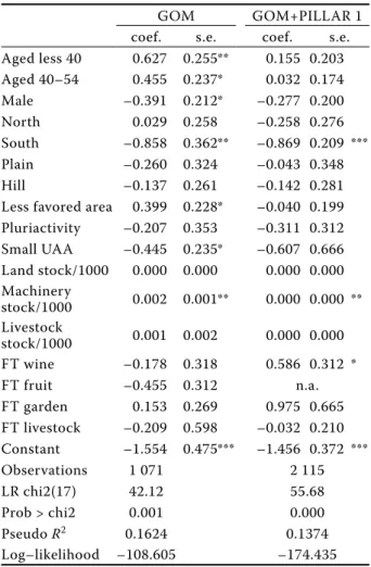
The parameter estimates of the probit equations are shown in Table 3. When focusing on farms only receiving support from GOMs, according to the age dummies, the probability of participating in the GOMs is higher for the young and middle-aged operators than for the elderly operators. This finding is consistent with our expectations. As anticipated, the probability of participating in GOMs is higher for female opera-tors and farms located in LFAs, while it is lower for farms located in the south and for small farms. Finally, machinery endowment positively affects participation. When looking at farms receiving benefits from both GOMs and pillar 1, we find that age and gender vari-ables have no significant effects, while the effects of location in the south and machinery endowment are significant and similar in magnitude to those found in the previous equation. In this second equation, we also find that farms specialising in wine are less likely to participate in GOMs.16
Table 3. Probit equation estimates
GOM GOM+PILLAR 1 coef. s.e. coef. s.e. Aged less 40 0.627 0.255** 0.155 0.203 Aged 40–54 0.455 0.237* 0.032 0.174 Male –0.391 0.212* –0.277 0.200 North 0.029 0.258 –0.258 0.276 South –0.858 0.362** –0.869 0.209 *** Plain –0.260 0.324 –0.043 0.348 Hill –0.137 0.261 –0.142 0.281 Less favored area 0.399 0.228* –0.040 0.199 Pluriactivity –0.207 0.353 –0.311 0.312 Small UAA –0.445 0.235* –0.607 0.666 Land stock/1000 0.000 0.000 0.000 0.000 Machinery stock/1000 0.002 0.001** 0.000 0.000 ** Livestock stock/1000 0.001 0.002 0.000 0.000 FT wine –0.178 0.318 0.586 0.312 * FT fruit –0.455 0.312 n.a. FT garden 0.153 0.269 0.975 0.665 FT livestock –0.209 0.598 –0.032 0.210 Constant –1.554 0.475*** –1.456 0.372 *** Observations 1 071 2 115 LR chi2(17) 42.12 55.68 Prob > chi2 0.001 0.000 Pseudo R2 0.1624 0.1374 Log–likelihood –108.605 –174.435 *significant at the 10% level; **significant at the 5% level; ***significant at the 1% level
Source: Authors’ elaboration of FADN data
16The robustness of the probit specification was checked by running various specification tests. These included a LR test
for the age linearity, which was rejected. Further, we ran many LR tests for the probit specification to test the stability of estimation results in the face of the inclusion of additional control variables. These tests rejected the significance of adding the interaction dummies between, in turn, age, gender, and territorial area. Additionally, we ran a LM test
Conditional difference-in-differences estimation of the ATT – GOMs only
In this section, we compare the effect of GOMs on a treated group constituted by farms receiving GOMs and an untreated one including farms not receiving any CAP measures. We report the esti-mation of the ATT according to nearest-neighbour matching in Table 4A17. The estimation results refer to the differences in the logarithms of the outcomes; hence, we are studying the impact of the GOMs on the growth rates of the outcomes. Specifically, the impact of the treatment on the treated farms is estimated by computing the mean differences across both groups.
The results do not show any statistically signifi-cant effect of participation in the GOMs on farm performance-related variables (gross output, em-ployment, farm income and partial productivities). As for the channels through which the investments affect the farm performance outcomes in the long run (land and machinery, capital stock, capital-land and capital-labour ratios), our findings show that while the control group is characterised by a reduction in both land (–5.4%) and machinery (–33.4%), the group of farms participating in the GOMs exhibit an increase in land capital (+4.5%) and a very minor disinvestment in machinery capital stock (–5.2%). The analysis also reveals that the treatment appears to counteract the
for normality after the probit that did not reject the null, while a score-test against heteroscedasticity revealed that the null of homoscedasticity was not rejected in many cases. Finally, testing revealed no difference in investment pro-pensity between treated and untreated farms. Brevity-related tables are not presented but are available upon request.
17Estimation results of the ATT according to the local linear regression confirm those according to nearest-neighbour
matching. They are available upon request.
Table 4A. CDID estimation results by 2 nearest-neighbour matching: GOM
Outcomes Sample Treated Controls Difference s.e. Bootstrap s.e. Δlog(FNAV) unmatchedATT 0.1540.134 0.1970.175 –0.043–0.041 0.1750.229 0.288 Δlog(FNAV/Capital) unmatched 0.162 0.129 0.033 0.192
ATT 0.153 0.218 –0.064 0.248 0.286 Δlog(FNAV/AWU) unmatchedATT 0.1890.150 0.2290.295 –0.040–0.145 0.1870.241 0.309 Δlog(FNAV/UAA) unmatchedATT 0.1090.103 0.2920.367 –0.182–0.265 0.1830.248 0.347 Δlog(AWU) unmatchedATT –0.025–0.033 0.0640.094 –0.090–0.127 0.0810.109 0.134 Δlog(PLV) unmatched 0.061 0.110 –0.049 0.106 ATT 0.051 0.103 –0.052 0.113 0.156 Δlog(Capital) unmatched 0.040 –0.091 0.131 0.067** ATT 0.028 –0.090 0.117 0.053** 0.083 Δlog(Capital/AWU) unmatched 0.066 –0.155 0.221 0.096** ATT 0.061 –0.183 0.244 0.114** 0.147* Δlog(Capital/UAA) unmatched 0.072 –0.056 0.128 0.067* ATT 0.040 –0.092 0.132 0.056** 0.076* Δlog(Land) unmatched 0.071 –0.072 0.143 0.087* ATT 0.045 –0.054 0.099 0.059* 0.118 Δlog(Machinery) unmatchedATT –0.060–0.052 –0.362–0.334 0.3020.282 0.140**0.132** 0.170* C(UAA/AWU) unmatched –0.006 –0.099 0.093 0.103
ATT 0.021 –0.092 0.112 0.114 0.165 *significant at the 10% level; **significant at the 5% level; ***significant at the 1% level; differences in the logarithms (Δlog ) correspond to growth rates
reduction in capital intensity observed in the control group producing a statistically significant positive impact on both the growth of capital-land (+4.0%) and capital-labour (+6.1%) ratios.
A specific issue in our analysis concerns the role of the GOMs in terms of capital/farm labour substitution or complementarity. Our estimation results can be interpreted as a test of both theses. AWU has declined for the treated and has increased for the untreated, resulting in a negative effect for the GOMs. However, as anticipated above, the estimations are not statisti-cally significant; hence, both these can be supported by our findings, and the possibility that the GOMs result in a substitution between capital and farm labour appears more probable than complementarity.
A further issue that we address is whether the out-comes depend on the volume of support. To take into account the effect of varying intensity in support, we
consider the distribution of funding received and identify the farms that receive an amount of support above the median, and then we repeat our evalu-ation on this sub-sample of farms18. As expected, it emerges that the farms receiving more support experienced a greater increase in the outcomes of interest. However, we also note that the causal effects are only statistically significant for those outcomes for which we have found a significant effect in the full sample of treated farms.
Conditional Difference-in-Differences estimation of the ATT – pillar 1 and GOMs
In this section, we replicate our investigation on a sample of farms all receiving pillar 1 payments and in which the treated group is composed of those farms also participating in GOMs. In other words, the causal effect is now estimated comparing a treated Table 4B. CDID estimation results by 2 nearest-neighbour matching: GOM+PILLAR 1
Outcomes Sample Treated Controls Difference s.e. Bootstrap s.e. Δlog(FNAV) unmatchedATT 0.3450.345 0.1220.112 0.2240.233 0.1490.189 0.250 Δlog(FNAV/Capital) unmatched 0.141 0.161 –0.020 0.143
ATT 0.141 0.150 –0.008 0.191 0.249 Δlog(FNAV/AWU) unmatched 0.292 0.093 0.199 0.152
ATT 0.292 0.039 0.253 0.194 0.260 Δlog(FNAV/UAA) unmatchedATT 0.2560.256 0.1180.097 0.1380.160 0.1470.193 0.261 Δlog(AWU) unmatchedATT 0.0530.053 0.0290.073 –0.0200.024 0.0790.092 0.119 Δlog(PLV) unmatched 0.358 0.094 0.264 0.084***
ATT 0.358 0.058 0.300 0.113*** 0.128 Δlog(Capital) unmatched 0.204 –0.039 0.243 0.051***
ATT 0.204 –0.038 0.242 0.070*** 0.096 Δlog(Capital/AWU) unmatchedATT 0.1510.151 –0.068–0.111 0.2190.262 0.081***0.084*** 0.136 Δlog(Capital/UAA) unmatchedATT 0.1150.115 –0.042–0.053 0.1580.168 0.045***0.059*** 0.073 Δlog(Land) unmatched 0.200 0.003 0.197 0.056*** ATT 0.200 –0.048 0.248 0.077*** 0.109 Δlog(Machinery) unmatched 0.247 –0.347 0.594 0.127*** ATT 0.247 –0.188 0.434 0.180*** 0.241 Δlog(UAA/AWU) unmatched 0.036 –0.025 0.061 0.084 ATT 0.036 –0.058 0.094 0.089 0.141 *significant at the 10% level; **significant at the 5% level; ***significant at the 1% level; differences in the logarithms (Δlog ) correspond to growth rates
Source: Authors’ elaboration of FADN data
group including farms receiving payments either from pillar 1 and GOMs, while the control group is composed of farms receiving only pillar 1 benefits. It is worth recalling that inclusion in the sample of farms receiving support from pillar 1 has a twofold effect. Firstly, given that a significant share of farms applied for and received pillar 1 payments, it almost doubles the size of the studied samples, in this way giving more robustness to the results of the analysis. Secondly, it deeply modifies the sample composition increasing the weight of farms specialising in products eligible for pillar 1 payments, namely arable crops, livestock and olives, in this way shifting the focus of the analysis away from Mediterranean crops, such as fruit, wine and horticultural crops.
Table 4B shows the estimation of the ATT accord-ing to nearest-neighbour matchaccord-ing19. Firstly, unlike the case in which farms do not benefit from pillar 1 support, we now find evidence of a statistically sig-nificant difference in the growth rate of gross output. More specifically, we find the gross output increase is 5.8% in the control group and 35.8% in treated farms. No statistically significant differences are found between the growth rates of net value added and employment in the two groups. Similar to the case described in the previous paragraph, we find that there is a statistically significant difference in the precursors to growth in the economic results. More specifically, we find a strong positive causal effect on the growth of land capital (+20.0%), machinery (+24.7%), capital-labour (+15.1%) and capital-land (11.5%) ratios in farms receiving both GOMs and pillar 1 support; in contrast, all these variables have negative signs in the control group.
DISCUSSION
Our results indicate that the participation in GOMs has had no significant effect on the differences in farm performance-related variables (gross output, employment, farm income and partial productivities) between treated and control farms. Our findings dif-fer from those of Medonos et al. (2012), while they
are in line with other papers that have investigated the link between investment and firm productivity beginning with the seminal work of Power (1998). This literature argues that while at the macroeconomic level there is a robust and and causal relationship between investment and long-run economic growth20 (De Long and Summers 1991), at the firm level in-vestment may have a negative effect on productivity in the short run. This is because investments usually imply the shut down and dismissing of old equip-ment, installation of new machinery and a loss of know-how and established routines. In “learning by doing” models, it takes some time for workers to learn how to use the new technology, and, as a consequence, labour productivity may rise to a higher level than the ex ante estimate only after a certain period of time. Nevertheless, our findings show that participation in the GOMs results in statistically significant differences between control and treated farms in the growth rates of the indicators of capital accumulation (land and machinery capital stock, as well as capital-land and capital-labour ratios). In this respect it is worth noting that we find farms in the control group to disinvest in the post-intervention period; in contrast, farms participating in GOMs increased both their capital endowment, due to investments in land improvement and equipment, and their capital intensity.
A related point to consider is that this difference in behaviour between treated and non-treated farms is already visible before the matching procedure, but it becomes larger after removing the systematic differ-ences between the treated and untreated observations, hence after correcting for self selection. The disin-vestment in non-treated farms is compatible with the structural change experienced in the farming sector in Italy in the fist decade of the present century. A very large decrease (–32.4%) in the number of farms was accompanied by a small decrease in utilised farm area (–2.5%) resulting in an unprecedented concentration of land in larger production units. By relaxing the capital credit constraint, investment support may have assisted the most dynamic farms in following an expansionary path.
19Estimation results of the ATT according to the local linear regression confirm those according to nearest-neighbour
matching. They are available upon request.
20The literature on endogenous growth that goes back to Romer (1986) assumes that investments and growth are
as-sociated through channels that make social returns higher than private ones. This positive externality is due to the increase in worker skills and in organisational competence arising from hands-on experience in using new technolo-gies and capital goods.
The increase in both capital endowment and capital intensity that we find in treated farms is expected to improve the farm’s performance in the long run, i.e., once the process of internal re-organisation is over. Firstly, the increase in capital endowment is expected to boost productivity, exploit economies of scale and lower production costs; hence, it should improve the farm’s performance in the long run. Although the real magnitude of economies of scale has been questioned (Goddard et al. 1993), it has still been shown that technological innovation is often biased in favour of large farms (Weiss 1999). Secondly, the increase in the intensity of capital per hour worked (hectare of land) signals that treated farms have activated a process of capital deepening. In endogenous growth theory, capital deepening is defined as a process that can lead to sustained eco-nomic growth even without technological progress because workers (land) become more productive when they have more and better capital to work with. Along this line of thinking, the estimated impact on capital intensity may be interpreted as a signal of activation of a channel through which in-vestment eventually impacts productivity and other farm performance-related variables. Consequently, even if no impact is found in the short term on the productivity and economic performance of partici-pating farms, yet we find the precursors of growth have been activated, and this finding is compatible with an improvement of a farm’s economic results in the long term.
CONCLUSIONS
A key issue in policy evaluation is the establishment of a baseline or counterfactual scenario to determine “additionality”, i.e., the additional net impact that a particular policy measure has had on the outcome of interest. In this paper, we applied a conditional difference-in-differences approach, where the treated and the untreated farms were matched on the basis of alternative matching methods to estimate the causal net effect of GOMs in the context of the RDP on selected farm outcomes.
The identification of the impact of GOMs may be problematic because of their interactions with other CAP measures. We tackled this problem by basing our analysis first on “pure” comparison and treat-ment groups: The first group contained farms that did not receive any programme intervention, either
from pillar 1 or 2, and the second group contained farms that only received GOM benefits. As a robust-ness check, we then replicated our investigation on a sample of farms all receiving pillar 1 payments, and compared the effects estimated for a treated group including farms receiving payments from either pillar 1 or GOMs to those estimated for the control group with farms receiving only pillar 1 support.
Our findings on the effects of participation in GOMs were not altered by the variation in samples; in other words, we estimated similar effects in farms receiving pillar 1 support and those not receiving it. In both investigations, we found no impact on farm income, employment or partial productivity. In this regard, it is important to recall that the one-year post-intervention period considered in this study might be too short to find a positive effect of the GOMs on the farm performance-related outcomes. When an investment is made, farms typically undergo reorganisation in the short run; as a consequence, their performance may improve only after the reorganisation is over. Nevertheless, both the analyses have demonstrated that farms participating in GOMs, in contrast to those not participating, experienced a positive sta-tistically significant impact on their land capital, a reduction in disinvestment in machinery capital stock, and, more notably, an increase in both their capital-land and capital-labour ratios. The increase in land is expected to lead to an increase in sales after a period of re-organisation, while the process of capital deepening activated by participation in GOMs is expected to result in a productivity increase in the long term and, eventually, in positive growth rates in farm performance. In other words, we argue that the estimated variations in land capital and the intensity of capital signal that the treatment resulted in the activation of channels that are expected to positively affect farm performance after a period of internal reorganisation.
Finally, the lack of statistically significant causal impacts on farm income and employment at the farm level in the short term cannot be directly interpreted as evidence of the ineffectiveness of the GOMs with respect to encouraging economic growth. Firstly, investments are a precondition to launch a process of experience and learning-by-doing, processes which increase an enterprise’s ability to produce efficiently. Secondly, apart from the increase in social returns, the estimated expansion and capital deepening in treated farms support the hypothesis of a positive impact even on private returns in the long term.
APPENDIX
Table A1A. Descriptive statistics of outcomes: GOM
Untreated (CSR) Treated
2007 2003 2007 2003
Outcomes mean Std Dev. mean Std Dev. mean Std Dev. mean Std Dev. FNAV 100 707 394 945 95 793 357 327 197 508 408 491 120 017 198 563 FNAV/capital 0.187 0.255 0.147 0.198 0.224 0.541 0.149 0.184 FNAV/AWU 23 361 25 586 27 658 85 806 40 188 70 434 23 604 20 065 FNAV/UAA 28 786 62 560 24 511 62 124 75 962 162 826 51 130 90 738 AWU 2.924 5.228 2.791 5.481 3.854 6.184 4.490 7.302 PLV 174 584 613 092 161 499 559 716 359 394 690 812 300 207 560 484 Capital stock 545 043 1 170 691 551 983 1 124 168 784 429 853 087 720 606 722 857 Land stock 435 565 1 028 236 430 807 936 358 535 686 475 880 485 487 408 111 Machinery stock 32 620 59 966 40 080 74 936 67 101 120 852 72 038 138 775 UAA/AWU 2.450 10.331 4.595 44.231 1.743 1.942 2.290 3.514 Capital/AWU 217 876 243 472 268 485 685 215 251 621 191 157 275 098 256 921 Capital/UAA 189 339 209 599 203 150 222 821 301 998 315 503 267 155 235 500 Source: Authors’ elaboration of FADN data
Table A1B. Descriptive statistics of outcomes: GOM+PILLAR 1
Untreated (CSR) Treated
2007 2003 2007 2003
Outcomes mean Std. Dev. mean Std. Dev. mean Std. Dev. mean Std. Dev. FNAV 74 437 179 127 66 108 176 293 184 776 273 992 118 491 149 279 FNAV/capital 0.08 0.08 0.07 0.07 0.08 0.10 0.05 0.06 FNAV/AWU 27 641 36 783 25 157 33 413 44 354 42 092 31 700 33 033 FNAV/UAA 2 022 3 148 1 883 3 244 3 698 5 799 2 093 2 375 AWU 2.22 3.29 2.05 2.74 3.76 5.75 3.11 2.61 PLV 134 033 296 515 119 400 274 141 330 044 383 745 225 008 253 735 Capital stock 975 511 1 759 363 969 514 1 672 964 3 276 321 7 207 333 2 143 324 2 432 883 Land stock 780 790 1 497 182 759 410 1 399 707 2 717 656 6 871 443 1 705 390 2 059 695 Machinery stock 49 462 74 387 60 009 82 118 169 202 179 865 126 423 120 863 UAA/AWU 20.78 28.50 23.08 43.09 26.71 27.45 24.14 21.26 Capital/AWU 449 686 589 157 485 625 821 168 709 012 459 957 600 532 383 285 Capital/UAA 27 869 21 936 28 569 22 562 46 578 40 704 41 579 38 381 Source: Authors’ elaboration of FADN data
REFERENCES
Ahituv A., Kimhi A. (2002): Off-farm work and capital accumulation decisions of farmers over the life-cycle: the role of heterogeneity and state dependence. Journal of Development Economics, 68: 329–353.
Benjamin C., Phimister E. (2002): Does capital market structure affect farm investment? A comparison using French and British farm-level panel data. American Journal of Agricultural Economics, 84: 1115–1129.
Blancard S., Boussemart J.P., Briec W., Kerstens K. (2006): Short-and long-run credit constraints in French agricul-ture: A directional distance function framework using expenditure-constrained profit functions. American Journal of Agricultural Economics, 88: 351–364. Caliendo M., Kopeinig S. (2008): Some practical guidance
for the implementation of propensity score matching. Journal of Economic Surveys, 22: 31–72.
Chabé-Ferret S., Subervie J. (2013): How much green for the buck? Estimating additional and windfall effects
of the French agro-environmental schemes by DID matching. Journal of Environmental Economics and Management, 65: 12–27.
Defrancesco E., Gatto P., Runge F., Trestini S. (2008). Factors affecting farmers’ participation in agri-envi-ronmental measures: A Northern Italian perspective. Journal of Agricultural Economics, 59: 114–131. Dehejia R., Wahba S. (2002): Propensity score matching
methods for nonexperimental causal studies. Review of Economics and Statistics, 84: 151–161.
De Long J.B., Summers L.H., Abel A.B. (1992). Equipment investment and economic growth: how strong is the nexus? Brookings Papers on Economic Activity, 1992: 157–211.
European Commission (2009): Rural Development (2000– 2006) in EU Farms. EC DGAGRI, Brussels.
Esposti R., Sotte F. (2013): Evaluating the effectiveness of agricultural and rural policies: an introduction. Euro-pean Review of Agricultural Economics, 40: 535–539. Goddard E., Weersink A., Chen K., Turvey C.G. (1993):
Economics of structural change in agriculture. Canadian Journal of Agricultural Economics/Revue canadienne d’agroeconomie, 41: 475–489.
Hazell P B., Poulto C., Wiggin, S., Dorwar A. (2007): The future of small farms for poverty reduction and growth. Discussion Paper 42, International Food Policy Research Institute, Washington.
Heckman J.J., Ichimura H., Todd P.E. (1997): Matching as an econometric evaluation estimator: evidence from evaluating a job training programme. The Review of Economic Studies, 64: 605–654
Heckman J.J., Ichimura H., Smith J., Todd P.E. (1998): Characterizing selection bias using experimental data, Econometrica. 66: 1017–1098.
Heckman J.J., Navarro-Lozano S. (2004): Using matching, instrumental variables, and control functions to estimate economic choice models. The Review of Economics and Statistics, 86: 30–57.
Kirchweger S., Kantelhardt J., Leisch F. (2015): Impacts of the government-supported investments on the economic farm performance in Austria. Agricultural Economics – Czech, 61: 343–355.
Medonos T., Ratinger T., Hruska M., Spicka J. (2012): The assessment of the effects of investment support measures of the rural development programmes: the case of the Czech Republic. AGRIS on-line Papers in Economics and Informatics, 4: 35–48.
Michalek J., Ciaian P., Kancs D. (2013): Firm-level evidence of deadweight loss of investment support policies: a case study of dairy farms in Schleswig-Holstein. In: IATRC
2013 Symposium: Productivity and Its Impacts on Global Trade, June 2–4, 2013, Seville.
Moro D., Sckokai P. (2011): The impact of pillar 1 sup-port on farm choices: conceptual and methodological challenges. In: 122nd EAAE Seminar, Feb 17–18, 2011,
Ancona.
OECD (2009): Methods to Monitor and Evaluate the Im-pacts of Agricultural Policies on Rural Development. OECD, Paris.
Ortner K.M. (2012): Evaluation of investment support in rural development programmes: results for selected measures. In: Cvijanović D., Floriańczyk Z. (eds): Rural Development Policies from the EU Enlargement Perspec-tive. ERDN book series, Rural areas and development, 9: 39–50.
Pascucci S., de-Magistris T., Dries L., Adinolfi F., Capi-tanio F. (2013): Participation of Italian farmers in rural development policy. European Review of Agricultural Economics, 40: 605–631.
Power L. (1998): The missing link: Technology, invest-ment, and productivity. The Review of Economics and Statistics, 80: 300–313.
Pufahl A., Weiss C.R. (2009): Evaluating the effects of farm programmes: results from propensity score matching. European Review of Agricultural Economics, 36: 79–101. Romer P.M. (1986): Increasing returns and long run growth.
Journal of Political Economy, 94: 1002–1037.
Rosenbaum P., Rubin D.B. (1983): The central role of the propensity score in observational studies for causal ef-fect. Biometrika, 70: 41–50.
Rosenzweig M.R., Binswanger H.P. (1993): Wealth, weather risk and the composition and profitability of agricultural investments. Economic Journal, 103: 56–78.
Smith J.A., Todd P.E. (2005): Does matching overcome La-londe’s critique of nonexperimental estimators? Journal of Econometrics, 125: 305–353.
Todd P.E. (2008): Evaluating social programs with endog-enous program placement and selection of the treated. In: Schultz T.P., Strauss J.A. (eds): Handbook of Devel-opment Economics, 4: 3847–3894.
Udagawa C., Hodge I., Reader M. (2014): Farm level costs of agri-environment measures: the impact of entry level stewardship on cereal farm incomes. Journal of Agri-cultural Economics, 65: 212–233.
Weiss C.R. (1999): Farm growth and survival: econometric evidence for individual farms in Upper Austria. Ameri-can Journal of Agricultural Economics, 81: 103–116.
Received March 3, 2016 Accepted June 19, 2017 Published online January 11, 2018