A business plan methodology modified to take advantage of data science

(1)

POLITECNICO DI MILANO

Scuola di Ingegneria Industriale e dell’Informazione

Corso di Laurea Magistrale in Ingegneria Informatica

A business plan methodology

modified to take advantage of

Data Science

Supervisor: Prof. Chiara Francalanci

Assistant Supervisor: Ing. Paolo Ravanelli

Master of Science Thesis of:

Alessandro Tribi

Student ID 804188

(2)

LIST OF FIGURES ... 4 LIST OF TABLES ... 5 ABSTRACT ... 7 SOMMARIO ... 8 1. INTRODUCTION ... 10 2. STATE OF THE ART ... 12 2.1 Open Data, Open Government and Open Government Data ... 12 2.1.1 Open Data History and Definition ... 12 2.1.2 Open Government ... 14 2.1.3 The benefits of Open Government Data ... 16 2.2 Data Analytics ... 18 2.2.1 Data Analytics Definition ... 18 2.2.2 Descriptive Analytics, Clustering and K-medoids ... 18 2.2.3 Predictive Analytics and Holt-Winters Method ... 21 2.2.4 Prescriptive Analytics ... 22 2.3 Previous works on Open Data about Road Accidents ... 23 2.3.1 Rome Open Data ... 23 2.3.2 United Kingdom Open Data ... 24 3. PROBLEM ANALYSIS ... 25 3.1 Data Retrieval and Preliminary Operations ... 25 3.1.1 UK Road Safety Data ... 26 3.1.2 Road Accidents Data of Rome ... 27 3.1.3 Other Data ... 27 3.1.4 Preliminary Operations on Data ... 28 3.2 Comparison between Rome and London ... 31 3.2.1 Car Drivers’ Age Differences ... 31 3.2.2 Trends for Young Drivers by Year and Vehicle Type ... 33 3.2.3 Trends for Young Car Drivers by Hour and Day of Week ... 35

(3)

3.3 Clustering on Rome’s Data ... 38 3.3.1 Data Pre-Processing ... 38 3.3.2 Choice of the Number of Clusters ... 43 3.3.3 Characteristics of the Clusters ... 45 4. METHODOLOGY ... 50 4.1 Executive Summary ... 54 4.2 Strategy ... 55 4.2.1 Identification of the Best Opportunity ... 56 4.2.2 Evaluation of the Best Opportunity: the Case Study about Pass Plus Extra ... 56 4.2.3 Evaluation of the Best Opportunity: Staffordshire’s Data Pre-Processing ... 61 4.2.4 Evaluation of the Best Opportunity: Clusters in Staffordshire’s Data ... 65 4.2.5 Evaluation of the Best Opportunity: Effects of Pass Plus Extra on Single Clusters ... 69 4.3 Analysis of Alternatives ... 73 4.4 Cost-Benefit Analysis ... 77 4.4.1 Possible Effects of Pass Plus Extra in Rome ... 77 4.4.2 Costs ... 79 4.4.3 Benefits ... 80 4.4.4 Results and Considerations ... 83 5. CONCLUSIONS ... 85 6. REFERENCES ... 87

(4)

LIST OF FIGURES

Figure 1 – PYTHON SCRIPT TO ACCESS WEATHER DATA ... 28 Figure 2 – PYTHON SCRIPT TO HANDLE JSON FORMATTING ERRORS 29 Figure 3 – NUMBER OF INVOLVED CAR DRIVERS BY AGE [Years:

2008-2014] ... 32 Figure 4 – NUMBER OF INVOLVED YOUNG DRIVERS BY VEHICLE AND

YEAR [Age: 18-22 Rome, 17-21 London] ... 34 Figure 5 – NUMBER OF INVOLVED YOUNG CAR DRIVERS BY HOUR

AND DAY OF THE WEEK [Rome, Years: 2008-2014] [Estimated_Age: 18-22] ... 36 Figure 6 – NUMBER OF INVOLVED YOUNG CAR DRIVERS BY HOUR

AND DAY OF THE WEEK [London, Years: 2008-2014] [Age: 17-21] ... 37 Figure 7 – AVERAGE SILHOUETTE WIDTH OF CLUSTERS IN ROME'S

DATA ... 44 Figure 8 – TRADITIONAL BUSINESS PLAN STRUCTURE ... 50 Figure 9 – MODIFIED BUSINESS PLAN STRUCTURE ... 52 Figure 10 – NUMBER OF INVOLVED CAR DRIVERS BY AGE BAND AND

REGION ... 58 Figure 11 – AVERAGE SILHOUETTE WIDTH OF CLUSTERS IN

STAFFORDSHIRE'S DATA ... 66 Figure 12 – NUMBER OF INVOLVED YOUNG CAR DRIVERS IN ROME BY

(5)

LIST OF TABLES

Table 1 – CLUSTERING METHODS CATEGORIES ... 20 Table 2 – DAILY RAINFALL CLASSES ... 39 Table 3 – AGGREGATIONS ON WEATHER CONDITIONS VALUES ABOUT

ROME’S DATA ... 40 Table 4 - AGGREGATIONS ON ROAD SURFACE CONDITIONS VALUES

ABOUT ROME’S DATA ... 41 Table 5 – AGGREGATIONS ON LIGHT CONDITIONS VALUES ABOUT

ROME’S DATA ... 41 Table 6 – AGGREGATIONS ON JUNCTION TYPE VALUES ABOUT

ROME’S DATA ... 42 Table 7 – CLUSTERS IN ROME'S DATA ... 47 Table 8 – COMPARISON STAFFORDSHIRE/REST OF ENGLAND ON THE

NUMBER OF INVOLVED YOUNG DRIVERS ... 60 Table 9 – NUMBER OF CLIENTS COMPLETING THE PASS PLUS EXTRA

PROCESS BY YEAR ... 61 Table 10 – AGGREGATIONS ON WEATHER CONDITIONS VALUES

ABOUT STAFFORDSHIRE'S DATA ... 62 Table 11 – AGGREGATIONS ON ROAD SURFACE CONDITIONS VALUES

ABOUT STAFFORDSHIRE’S DATA ... 63 Table 12 – AGGREGATIONS ON LIGHT CONDITIONS VALUES ABOUT

STAFFORDSHIRE'S DATA ... 63 Table 13 – AGGREGATIONS ON JUNCTION TYPE VALUES ABOUT

STAFFORDSHIRE’S DATA ... 64 Table 14 – COMPARISON STAFFORDSHIRE/REST OF ENGLAND ON THE

TREND OF THE CLUSTER 5 ... 70 Table 15 – COMPARISON STAFFORDSHIRE/REST OF ENGLAND ON THE

(6)

Table 16 – COMPARISON STAFFORDSHIRE/REST OF ENGLAND ON THE TREND OF THE CLUSTER 12 ... 71 Table 17 - COMPARISON STAFFORDSHIRE/REST OF ENGLAND ON THE

TREND OF THE CLUSTER 13 ... 73 Table 20 - HYPOTHESES ON THE MAIN CAUSE OF THE ISSUE ABOUT

YOUNG CAR DRIVERS INVOLVED IN SERIOUS CRASHES IN ROME ... 75 Table 21 – NUMBER OF POTENTIALLY SAVED YOUNG CAR DRIVERS IN

ROME ... 79 Table 22 – POTENTIAL COSTS FOR THE LOCAL AUTHORITY IN ROME 80 Table 23 – POTENTIALLY SAVED SOCIAL COSTS IN ROME ... 82 Table 24 – ANNUAL POTENTIAL COSTS AND BENEFITS FOR ROME ... 83

(7)

ABSTRACT

In the last recent years, Data Science has been widely employed by companies and governments to turn data into insight for making better decisions. In par-ticular, concerning the public sector, this phenomenon has acquired increasing importance since 2007, when the eight principles of Open Government Data have been defined. These data are produced or commissioned by public bodies and they are made freely accessible and usable by everyone.

The aim of this work is to propose a revised methodology for writing a business plan, in order to take advantage of Data Science. This methodology is then used to write a business plan about the proposal for a road safety action. The action is intended for Rome, where, after having performed an analysis on data about road accidents, a serious issue regarding young drivers has been revealed. Rome has an extremely high number of young car drivers involved in personal injury accidents. The value is even more evident if compared to London.

A more detailed study on the data has allowed to identify the risky driving as the cause of the problem. For this reason, a case study showing a solution to a similar problem has been searched and it has been identified in Staffordshire, a county of the United Kingdom. In this region, after the introduction of an en-hanced driving course, which is called Pass Plus Extra and it aims to increase the road safety awareness, a strong fall in the number of young drivers involved in serious crashes has been achieved. After having evaluated the effectiveness of the course by means of Data Science techniques, the economic and social ad-vantages that the introduction of a similar enhanced driving course would have caused in Rome in the last four years have been estimated and the results are extremely positive. The innovative methodology presented in this work is sup-posed to be suitable not only in this case, but also in all the other contexts in which complete and updated data are available.

(8)

SOMMARIO

Negli ultimi anni, la scienza dei dati (Data Science) è stata largamente impie-gata da imprese e governi per trasformare i dati in informazione utile, in modo da poter prendere le decisioni migliori. In particolare, per quanto riguarda il settore pubblico, questo fenomeno ha acquisito sempre maggior importanza a partire dal 2007, quando sono stati definiti gli otto principi dei dati governativi aperti (Open Government Data). Questi dati sono prodotti o commissionati da enti pubblici e vengono resi liberamente accessibili e utilizzabili da tutti.

Lo scopo di questa tesi è proporre una metodologia di redazione di studio di fat-tibilità modificata, per trarre vantaggio dalla Data Science. Questa metodologia viene poi utilizzata per redigere uno studio di fattibilità riguardante la proposta di attuazione di un intervento per la sicurezza stradale. L’intervento riguarda la città di Roma, dove, in seguito all’analisi dei dati riguardanti gli incidenti stradali, è stato rivelato un aspetto preoccupante relativo ai giovani conducenti. Roma, infatti, presenta un numero estremamente alto di giovani conducenti di automobili coinvolti in incidenti stradali con danni a persone. Il dato è ancor più evidente se paragonato a quello di Londra.

Uno studio più approfondito sui dati ha permesso di identificare come causa del problema la guida pericolosa dei giovani conducenti di Roma. Per questo motivo, si è cercato un caso di studio che presentasse una soluzione ad un problema simile ed è stato individuato nello Staffordshire, una contea del Regno Unito. In questa regione, in seguito all’introduzione di un corso di guida avanzata, chia-mato Pass Plus Extra e improntato a migliorare la consapevolezza dei rischi legati alla guida, è stato registrato un netto calo del numero di giovani condu-centi coinvolti in gravi incidenti. Dopo aver valutato l’efficacia del corso tramite tecniche di Data Science, sono stati stimati i vantaggi economici e sociali che l’introduzione di un simile corso di guida avanzata avrebbe portato a Roma negli ultimi quattro anni e i risultati sono estremamente positivi.

(9)

Si ritiene che la metodologia innovativa presentata in questa tesi non sia appli-cabile solo al caso in esame, ma anche in tutti gli altri contesti in cui si abbiano a disposizione dati completi e aggiornati.

(10)

1. INTRODUCTION

The concept of Open Data has acquired great importance in the last few years. In some countries, like the United Kingdom and the United States of America, they are regularly analysed and investigated to detect possible issues or identify new opportunities. In these countries, not only private companies, but also gov-ernments and local authorities are taking advantage of the great potentiality of open data. The same can’t be argued about Italy, where the open data manage-ment still presents some evident lacks and it could be highly improved.

One of the few examples of an updated Italian open data portal containing in-teresting information is represented by the official portal of Rome. This work starts from data about road accidents taken from this open data portal and data about the same topic taken from the national open data portal of the United Kingdom. Then, a comparison between Rome and London is performed and a serious issue for Rome is identified, which is the extremely high number of young drivers involved in personal injury accidents. Finally, inside a completely revised business plan structure, conceived to take advantage of data science, a possible remedy is found, the quick fix action is evaluated and the economic and social impact that it would have had, if it had been applied in Rome four years ago, is precisely calculated.

The most innovative aspect of this work is represented by the proposal of an innovative methodology for the realisation of a business plan, based on the huge potentiality of data science. The business plan is related to the possible intro-duction of a road safety action and a fundamental role is held by open data and data science techniques, as they are used to get extremely precise results that aren’t achievable by traditional approaches in this area. In fact, all the actions

(11)

1. INTRODUCTION

taken up to now in the road safety field in Italy have been based on and evalu-ated by general statistics. One of the main shortcomings of this type of studies is that they can’t describe in detail the features of an issue and the consequences of a public intervention.

The structure of the work is the following.

In chapter 2, as a result of a literature review, the state of the art of open data, open government, data analytics and works on open data about road accidents is provided.

In chapter 3 all the operation needed to retrieve and analyse open data are scribed. Then, a comparison between Rome and London is performed and a de-tailed qualitative analysis of the issue about young road casualties in Rome is produced.

In chapter 4 a modified version of the classic business plan structure is shown. This structure, revised to take advantage of data science, is then used to write a business plan about a possible road safety action in Rome.

(12)

2. STATE OF THE ART

In this chapter the main topics covered in this work are presented. Their state of the art, resulted from a literature review, is described. The following themes are treated: open data, open government and open government data (section 2.1), data analytics (section 2.2) and previous works on open data about road accidents (section 2.3).

2.1 Open Data, Open Government and Open Government

Data

This section introduces the concepts of Open Data, Open Government and Open

Government Data, by mentioning some relevant historical facts and giving some

useful definitions and information.

2.1.1 Open Data History and Definition

Robert King Merton, an American sociologist, was the first one who theorized that knowledge has to be shared for the common good. In his essay “The

Norma-tive Structure of Science”, published in 1942, he described the modern science as

a community in which the scientists’ behaviour should be controlled by four norms: universalism, “communism” (later renamed as communalism), disinter-estedness and organized scepticism. According to the second norm, in particular, the scientific knowledge is identified as a common property and it’s argued that

(13)

2.1 Open Data, Open Government and Open Government Data

the results of scientific researches should be freely accessible to everyone, in order to let the science and the knowledge grow. [15]

The birth of the new information technologies, among which Internet has defi-nitely had a crucial impact, led to more and more considerations about knowledge sharing and therefore data sharing.

In 2004 the Open Knowledge Foundation, a global non-profit network, was founded. Their mission is well illustrated by their own words:

“We envision a world where:

• knowledge creates power for the many, not the few.

• data frees us to make informed choices about how we live, what we buy and

who gets our vote.

• information and insights are accessible – and apparent – to everyone.” [12] They released the first version of the Open Definition in 2005 and it is main-tained today by an Advisory Council. The definition identifies the characteristics that data must have to be recognized as open:

“To summarize the most important:

• Availability and Access: the data must be available as a whole and at no more

than a reasonable reproduction cost, preferably by downloading over the in-ternet. The data must also be available in a convenient and modifiable form.

• Re-use and Redistribution: the data must be provided under terms that

per-mit re-use and redistribution including the intermixing with other datasets.

• Universal Participation: everyone must be able to use, re-use and redistribute

- there should be no discrimination against fields of endeavour or against persons or groups. For example, ‘non-commercial’ restrictions that would pre-vent ‘commercial’ use, or restrictions of use for certain purposes (e.g. only in education), are not allowed.” [13]

(14)

2. STATE OF THE ART

Nowadays there are several fields in which open data are used (for instance government, science, economics, etc.). If open data are produced or commis-sioned by public bodies, they are called Open Government Data.

In December 2007, thirty open government advocates defined the 8 principles of Open Government Data. Public government data shall be considered open if they are:

• Complete – “All public data is made available. Public data is data that is not

subject to valid privacy, security or privilege limitations.”

• Primary – “Data is as collected at the source, with the highest possible level

of granularity, not in aggregate or modified forms.”

• Timely – “Data is made available as quickly as necessary to preserve the value

of the data.”

• Accessible – “Data is available to the widest range of users for the widest

range of purposes.”

• Machine processable – “Data is reasonably structured to allow automated

processing.”

• Non-discriminatory – “Data is available to anyone, with no requirement of

registration.”

• Non-proprietary – “Data is available in a format over which no entity has

exclusive control.”

• License-free – “Data is not subject to any copyright, patent, trademark or

trade secret regulation. Reasonable privacy, security and privilege restrictions may be allowed.” [16]

2.1.2 Open Government

In order to explain the concept of Open Government, it is worth starting from the “Memorandum on Transparency and Open Government”, signed by the Pres-ident of U.S.A. Barack Obama on January 21, 2009. It contains the three main

(15)

principles upon which all Open Government initiatives taken by other countries since then are based.

The principles are the following:

“Government should be transparent. Transparency promotes accountability and provides information for citizens about what their Government is doing. [...] Government should be participatory. Public engagement enhances the Govern-ment's effectiveness and improves the quality of its decisions. Knowledge is widely dispersed in society, and public officials benefit from having access to that dispersed knowledge. […] Executive departments and agencies should also solicit public input on how we can increase and improve opportunities for public par-ticipation in Government. […]

Government should be collaborative. […] Executive departments and agencies should use innovative tools, methods, and systems to cooperate among them-selves, across all levels of Government, and with nonprofit organizations, busi-nesses, and individuals in the private sector. Executive departments and agencies should solicit public feedback to assess and improve their level of collaboration and to identify new opportunities for cooperation.” [11]

Thus, the concept of Open Government is closely related to the concept of Open

Government Data mentioned above.

United Kingdom and Italy, like other several countries, have been inspired by this memorandum. The former published the report “Putting the frontline first:

smarter government” in December 2009, in which it was stated that one of the

key action of the new plan was to “radically open up data and public information

to promote transparent and effective government and social innovation” and it

was announced the release of over a thousand public datasets made free for re-use. [7] In January 2010 the official Open Data portal of the UK Government (data.gov.uk) launched publicly and now it contains thousands of datasets about

(16)

2. STATE OF THE ART

different themes, among which environment, health, transport, education and society.

The latter joined the Open Government Partnership in September 2011, an in-ternational organization that looks for strong commitments from each member country to promote transparency and empower citizens by taking advantage of new technologies. The partnership currently includes 69 participating coun-tries.

In April 2012 Italy summarized its programs and initiatives in an Action Plan and subsequently the Italian Open Data portal launched (dati.gov.it). After more than three years, the portal still has a big problem: most of the data are not updated, they belong to datasets placed into the portal and then forgotten, so they can’t be considered interesting and they seem to go against the Open Government principles. [8]

Not only national Open Data portals were born in these years, but also local authorities launched their own ones. The portal of the city of Rome (dati.co-mune.roma.it) has been used in this work and so it deserves to be cited. Launched on October 3, 2012, now it contains plenty of data about 11 different areas, among which tourism, road accidents, environment, society and public administration. The data are continuously updated, for this reason they are a very good resource for people who want to get useful information from them.

2.1.3 The benefits of Open Government Data

Open Government Data can be searched and manipulated using standard tools, each citizen with basic knowledge of Information Technology can exploit them and, potentially, create value from them. The main beneficiaries of the value created from these data are: government, citizens and wider economy.

(17)

They improve transparency and accountability, they produce innovative and personalized public services and they enhance the interaction processes between citizens and government. [17]

The release of government data online and their reuse can lead to a considerable decrease of the number of questions daily received by public authorities. This produces a reduction in work-load and costs and makes easier for public employ-ees to answer to the remaining questions, because necessary information is also faster to find. A good example of what has just been stated is the case of the Netherlands, where the Ministry of Education has published education-related data for reuse and this has significantly improved the efficiency of the relative public services. [13]

Citizens – The publication of Open Government Data is obviously considered an

important and innovative service for citizens: it increases the public participa-tion and it gives more responsibilities to the public authority, as everyone can verify how it is working. [17] In Finland and in the United Kingdom, just to give an idea, there are two projects, respectively called “tax tree” and “where does my money go”, that let the people know how the government spends tax money. Moreover, people can make better decisions in their own life, there are plenty of examples of new mobile apps and new services built upon Open Government Data. For example, they can help in finding the best place to live (like

mapu-mental.com in the UK and mapnificent.net in Germany), the nearest place where

it is possible to walk the dog or even the nearest public toilet (like findtoilet.dk in Denmark). [13]

Wider economy – According to the Open definition, open data can be used for

commercial purposes. It’s a proven fact that, if it’s allowed the reuse of some data at very low or zero cost, developers and private enterprises can take ad-vantage of this information and create more and more products to be marketed. As a consequence, national economy is strengthened and the government can receive revenue in the form of taxes. [17]

(18)

2. STATE OF THE ART

2.2 Data Analytics

In this section Data Analytics and the three categories in which it can be divided are presented. Data Analytics covers a huge number of methods and techniques. Two of them, the Clustering technique and the Holt-Winters method, have been used in this study and therefore a brief explanation of them is provided too.

2.2.1 Data Analytics Definition

Data Analytics is the science of analysing raw data in order to transform these

data into insight and make better business decisions.

Thanks to the very useful information and knowledge it gives to the managers, its popularity has extremely increased in the last years and now a new concept has been introduced in the business world: analytics-as-a-service. This term re-fers to the utilization of web-delivered technologies for performing Data Analyt-ics, in order to take advantage of as-a-service characteristAnalyt-ics, like pay-per-use and high scalability.

Data Analytics is divided into three main categories: Descriptive Analytics, Pre-dictive Analytics and Prescriptive Analytics.

2.2.2 Descriptive Analytics, Clustering and K-medoids

“What happened?”

Descriptive Analytics focuses on the past. It takes as input data regarding what happened until now, it summarizes them and it tries to discover interesting in-formation that can be useful for describing a problem or determining opportuni-ties, it can illustrate a scenario in which it’s possible to take advantage of that

(19)

2.2 Data Analytics

Statistics (sums, averages, etc.), reports about historical facts and transactions and every other technique that aggregates raw data and make them interpret-able by humans belong to this category. [3]

One of the most used technique is clustering. The main task of clustering (or

cluster analysis) is to find similarities between data and divide them into

differ-ent groups, so that data objects inside the same cluster are similar to each other and dissimilar to objects belonging to the other groups.

There are a lot of different algorithms able to perform this action and there isn’t an algorithm that can always be defined as the best one, each algorithm could be the most appropriate to be used for every specific case. It depends on the type of the data (they can be numeric, ordinal, binary, categorical), the data charac-teristics (for instance high/low number of outliers or missing values) and the algorithm characteristics that are needed (it can be more/less scalable or easy/hard to be interpreted).

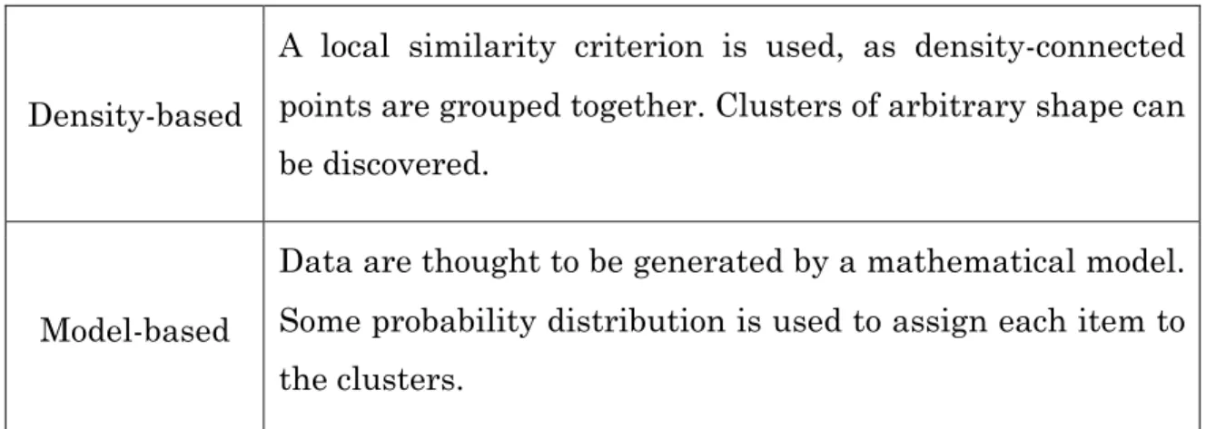
Moreover, clustering methods can be divided into 4 categories, depending on how they work. The categories are:

Hierarchical

Initially, groups are composed by an element. Then, at each step, the most similar groups are merged together, until a single group is obtained (or, on the contrary, the algorithm starts from a cluster containing all data objects and, at each step, it splits up one group until each cluster is composed by a single item).

Partitioning

Given k clusters, the algorithm assigns each data object to a cluster, trying to obtain a result in which items of the same group have high similarity.

(20)

2. STATE OF THE ART

Density-based

A local similarity criterion is used, as density-connected points are grouped together. Clusters of arbitrary shape can be discovered.

Model-based

Data are thought to be generated by a mathematical model. Some probability distribution is used to assign each item to the clusters.

Table 1 – CLUSTERING METHODS CATEGORIES

After an algorithm has finished its execution, usually, an evaluation of its re-sults is performed. Based on intra-class and inter-class similarity, it is possible to choose the number of clusters that better represents the data.

A clustering problem that is worth examining in depth, as it has been analysed in this study, is called k-medoid. It refers to the class of the partitioning methods and its goal is to minimize the distance between the elements of each cluster and the item that represents the most central point (medoid) of that cluster. The most used and famous algorithm for finding a solution (a local minimum) to the k-medoid problem is the PAM algorithm (Partitioning Around Medoids). It can work with the dissimilarity matrix, that is a matrix containing all the pairwise distances between the items, or directly with the data, by calculating the distance matrix it needs at first. It is composed by two phases: the build phase and the swap phase.

During the build phase, the observation whose sum of dissimilarities is mini-mum is chosen as the first medoid. Then, the other k-1 initial medoids are se-lected iteratively by minimizing the distance of the other data objects to their nearest medoid.

At the end of the build phase, k initial medoids are obtained and the swap phase begins. The algorithm swaps each selected medoid with a non-selected object

(21)

2.2 Data Analytics

medoid decreases, then a new configuration has been found. The process contin-ues until no further optimization is possible.

The final k medoids are the objects that best represent their own cluster and all the other observations are assigned to the cluster whose medoid is more similar to them.

2.2.3 Predictive Analytics and Holt-Winters Method

“What will happen?”

Here the focus is on the future. As the word predictive suggests, Predictive An-alytics uses associations between data and trends to determine how a phenom-enon is going to proceed in the future. [3]

Data mining, text mining and machine learning techniques belongs to this cat-egory, but also statistical time series forecasting is very popular. In general, each model and each technique that takes data about the past to predict future data is considered as part of Predictive Analytics.

The method used in this study is called Holt-Winters method, it performs time series forecasting and it is used when there is seasonality in the data. There are two versions of the method: the additive method and the multiplicative one. The former is preferred when the variations are roughly constant in the series, the latter is better when the variations change proportionally to the level of the se-ries and therefore it’s worth considering the percentage of the variations.

Both of them are comprised of 4 equations, the first one represents the forecast equation and the other ones are needed to calculate the estimated level [𝑙"],

trend [𝑏"] and seasonal component [𝑠"] at time t. The equations of the additive

model, which is the model that has been used here, are: 𝑌_"&' = 𝑙_"+ ℎ𝑏_"+ 𝑠_{",-&.& ',.} /01 -𝑙 = 𝛼 𝑌 − 𝑠 + (1 − 𝛼)(𝑙 + 𝑏 )

(22)

2. STATE OF THE ART

𝑏_"= 𝛽 𝑙_"− 𝑙_",. + (1 − 𝛽)𝑏_",. 𝑠_"= 𝛾 𝑌_"− 𝑙_",.− 𝑏_",. + 1 − 𝛾 𝑠

",-where ℎ = 1, 2, … represents the number of steps ahead into the future (starting from the last observation we have) and 𝑝 stands for the period length of the seasonality (for instance, monthly data has 𝑝 = 12). 𝛼, 𝛽 and 𝛾 are called

smooth-ing parameters. They are needed to calculate the weighted average inside their

respective equations and they can be specified by the forecaster or obtained from the observed data. In this case the values that minimize the sum of the squared errors (and therefore maximize the forecast accuracy) are chosen.

In the first equation, the h-step ahead forecast is obtained by adding the level at time t, the trend component and the seasonal index taken from the last year of the observations. The level is calculated as a weighted average between the observation without its seasonality and the non-seasonal forecast for time t. The weighted average inside the trend equations makes use of the difference be-tween the last two levels and the previous value of trend. Lastly, the seasonal index is calculated as a weighted average between the current seasonal index and the index that refers to the same season in the previous year.

2.2.4 Prescriptive Analytics

“What should I do?”

The goal of Prescriptive Analytics is to find the best actions to improve the cur-rent situation. Typically, a Data Analytics expert shows to a manager some pos-sible scenarios, better than the current one, in which the company could be placed in the future and the actions needed to reach that situation. This is ob-tained after the execution of some mathematical algorithm on the provided data, based on constraints and requirements given as input.

(23)

2.3 Previous works on Open Data about Road Accidents

Prescriptive Analytics, together with managers’ experience, can get the best course of action for each particular situation and let the company reach its ob-jectives. [3]

2.3 Previous works on Open Data about Road

Acci-dents

This part describes how open data about road accidents have been analysed by previous works and researches so far. The focus is on accidents occurred in Rome and in the United Kingdom, the two cases covered by this work.

2.3.1 Rome Open Data

So far, the only works based on Rome’s open data about road accidents are web-sites and applications that provide a map visualization of the crashes. This is probably due to the fact that open data have appeared in Italy very recently and their enormous potential has not been fully exploited yet.

An example of what has just been stated could be “Roma Crash Map”, a visual-ization tool, developed some years ago, able to show the density of car accidents in the different Rome municipalities, also by grouping them according to their characteristics, such as light conditions, weather conditions and periods of time.

(24)

2. STATE OF THE ART

2.3.2 United Kingdom Open Data

There are several websites containing map visualization tools that work on data taken from the UK open data portal. http://www.cyclestreets.net/collisions/ and http://www.crashmap.co.uk are just two examples of this category.

Both show a map in which the user can detect the exact position of all road accidents from 2008 to 2014 and they also provide some information about each single crash. Three different types of markers, distinguished by their colour (ranging from yellow to red), differentiate between accidents with slight, serious and fatal consequences.

The former website focuses on accidents involving cyclists. The latter lets the user filter crashes by the location, the year in which they took place, their se-verity and the types of casualties.

However, it’s worth paying close attention to the researches conducted on crashes open data. They are often commissioned by public authorities and their goal is to find some interesting aspects that can help in improving road safety. One of the most recent one was published in March 2015 and commissioned by the Welsh Government. Its purpose was to evaluate the effects of the Pass Plus Cymru, a course designed to improve young drivers’ skills. In addition to con-sultations with people from the road safety staff and a careful literature review to analyse the impact of other similar courses, the researchers took in consider-ation several statistics based on data from the UK open data portal. [14]

(25)

3. PROBLEM ANALYSIS

This chapter focuses on the analysis of the data about drivers involved in per-sonal injury accidents in Rome and in London. In particular, the first section explains all the operations performed to get the data that have been used and make them ready to be examined by a data analytics tool. In the second section a comparison between Rome and London is shown by means of analyses on spe-cific attributes and a problem relating to young drivers in Rome comes to light. Finally, the third section illustrates the implementation of a clustering analysis on Rome’s data and the obtained results. These are used to better describe the characteristics of the issue about young drivers involved in car accidents in Rome.

All data analyses have been performed by using the R software and its libraries.

3.1 Data Retrieval and Preliminary Operations

This work is based on data about road accidents taken from two open data por-tals. The first one is the official open data portal of the United Kingdom Govern-ment and road safety data can be found at

https://data.gov.uk/dataset/road-accidents-safety-data. The second one is the open data portal of the city of Rome

and the webpage from which it’s possible to download data about road accidents is http://dati.comune.roma.it/cms/it/incidenti_stradali.page.

Moreover, data about daily rainfall in Rome and data about the population of Rome and the population of London are used. Daily rainfall data are taken from the open data portal of the Lazio region and precisely from

(26)

3. PROBLEM ANALYSIS

of Rome can be found at

http://dati.comune.roma.it/cms/it/popolazione_so-cieta.page and the estimates of the population of London are taken from the

Office for National Statistics (ONS) website, http://www.ons.gov.uk.

In the following paragraphs the main characteristics of the data found in these datasets are presented. Then, a brief explanation of the operations needed to make these data ready to be investigated by data analytics tools is provided.

3.1.1 UK Road Safety Data

The data are provided in CSV format and they belong to STATS19 database, which is a collection of personal injury road accidents that took place in Great Britain from 1979. The data about accidents from 2005 and 2014 are more pre-cise about the age of the drivers, as they include the exact age. For this reason, they have been used in this work. Previous data, instead, only provide infor-mation about five-year and ten-year age bands.

There are three different datasets: Accidents, Vehicles and Casualties. Only the first two of them have been taken into account, because they are useful for the purposes of this study.

Moreover, a document that acts as a data guide is provided. It contains tables specifying the meaning of each value associated to the variables.

In order to better understand the differences between the values of a certain variable, the STATS20 manual has also been used. It explains in detail all the information a Police Officer has to gather when a road accident resulted in a personal injury is reported. The manual can be found at the following link:

https://www.gov.uk/government/uploads/system/uploads/attach-ment_data/file/230596/stats20-2011.pdf.

(27)

3.1 Data Retrieval and Preliminary Operations

3.1.2 Road Accidents Data of Rome

The data taken from the portal of Rome are of two different formats: JSON and XML. JSON data are the most recent and updated ones, but they lack infor-mation about accidents occurred on June 30 and December 31 for each year, so XML data regarding these two days need to be employed too.

Four different datasets are provided: Accidents, Vehicles, Persons and Pedestri-ans. The first three of them have been used in this work and the time interval considered is between January 2008 and June 2015, data regarding periods of time after this point are not available yet.

Each single dataset covers a period of six months inside this time interval.

3.1.3 Other Data

The data about the population of Rome and London can be directly downloaded from their respective websites and they are contained in CSV files.

In order to get the daily rainfall data from the open data portal of the Lazio region, instead, it is necessary to write and run a script able to access to the remote resources and export JSON data. These data, then, are saved to a JSON file. There is one weather dataset per year and each dataset is identified by an id, which is needed to access the resource. The script, written in Python lan-guage, is the following.

(28)

3. PROBLEM ANALYSIS

Figure 1 – PYTHON SCRIPT TO ACCESS WEATHER DATA

It selects data regarding the total daily rainfall (“PREC_TOTG”) registered by two weather stations of Rome, “ROMA Lanciani” and “ROMA Ponte Nona”. The former station is taken as the primary source of data, because it is the nearest to the centre of Rome, but it lacks information about ten days for the entire period from January 2008 to June 2015, hence data from the latter station are taken into account for these specific days. The additional info about how many weather observations are needed (up to 6,000) has to be included because, oth-erwise, only a part of them are sent back in the response.

3.1.4 Preliminary Operations on Data

Files containing UK road safety data, data about daily rainfall in Rome and data about the population of Rome and London can directly be read by the R tool, as there aren’t any obstacles to the creation of data frames for these data.

On the contrary, as it has been stated before, the data about road accidents in Rome present some problems.

(29)

3.1 Data Retrieval and Preliminary Operations

First of all, two different formats (JSON and XML) have to be considered, so, in order to obtain the final data frame to be used, observations taken from files in both formats are required.

In addition, some fields of the JSON data contain strings taken “as is” from user input and not all these strings can be considered valid JSON strings. There are several cases, in fact, in which special characters, such as the double quotation mark (“) and the backslash (\), are not preceded by the escape character, which is the backslash itself. Each string having this issue cannot be accepted as valid inside a JSON structure. In order to solve this situation, an other script has been written in Python language and it has been run for every dataset having the issue.

The following script handles the dataset about road accidents occurred in Rome in the first six months of 2014.

Figure 2 – PYTHON SCRIPT TO HANDLE JSON FORMATTING ERRORS

For each line of the JSON file, a pattern is searched. The pattern makes use of a regular expression: the sequence of symbols (.+) indicates a string with length greater than zero placed between the substring on the left and the substring on

(30)

3. PROBLEM ANALYSIS

the attribute DaSpecificare, which is followed by the attribute NaturaIncidente inside the JSON file.

When such a string is found, it is passed to the variable substring

(re-sult.group(1) refers to the searched string) and, if it contains backslashes or

dou-ble quotation marks, an escape character is placed on their left. Every time a backslash character is written inside a Python string, it has to be expressed by two backslashes, because otherwise its role of escaping character is taken into account. After this operation has been completed, the line is reconstructed and it can be written on the output file.

Once these operations have been completed, all data can be imported into R (R libraries “jsonlite” and “XML” have been used) and stored into different data frames. Then, data frames containing observations of the same type but regard-ing different time periods need to be aggregated into sregard-ingle data collections. Fi-nally, the data frames Accidents and Vehicles about UK data are joined to obtain the final single data frame containing UK observations. The same is done with the the data frames regarding accidents, vehicles, people and daily rainfall about Rome.

As a last remark, it’s worth specifying that not all the observations about Rome’s accidents have been confirmed: a few of them present the logical value False for the attribute CONFERMATO and, thus, they have not been taken into account in this work. They typically represent unrevised copies of existing observations or partial data with several missing values that have been inserted into the da-taset by mistake.

(31)

3.2 Comparison between Rome and London

Among the data about accidents in the United Kingdom, the observations re-garding the crashes in London have been considered, because London is the city with the most similar features compared to Rome and, then, it can be used to make a valid comparison and find the specific characteristics of the accidents occurred in Rome.

London is identified by 34 different values of the attribute

Local_Author-ity_.Highway. inside the UK dataset: one corresponds to the Heathrow airport

and the code is “EHEATHROW”, the remaining 33 values correspond to the 33 districts (or boroughs) into which London is divided and all the codes related to them begin with “E09”.

3.2.1 Car Drivers’ Age Differences

As a first comparison between Rome and London, the car drivers’ age differences have been investigated. The Age_of_Driver is present as attribute in the UK data, while data about accidents occurred in Rome only provides the year of birth. Therefore, what can be done is to calculate the difference between the year in which the accident took place and the year of birth and the result represents a good estimate of the driver’s age (actually it could be the exact age or it could be wrong by one year, by considering the driver as one year older). From now on this value will be called Estimated_Age for convenience and it will be considered as a further variable of Rome’s data.

In addition, the value “Car” inside the Vehicle_Type attribute of the UK data, refers both to cars and light quadricycles and there is no way to distinguish between them. Among the “Instructions for the Completion of Road Accident

Re-ports” it is specified that the term “Car” includes each type of car “and similar four-wheel drive vehicles”. [4] For this reason, in order to make UK data as much

(32)

3. PROBLEM ANALYSIS

as possible comparable to Rome’s data, the vehicle types “Autovettura privata” (car) and “Quadriciclo leggero” (light quadricycle) have been taken into account for Rome’s observations. Actually, data regarding light quadricycles seem to be little relevant for the comparison, as only the 1.1% of the car drivers analysed, in the case of Rome, refers to light quadricycles.

In order to select only data about drivers, the value “Conducente” of the attribute

TipoPersona has been specified.

The time period between January 2008 and December 2014 has been considered, as data from both data frames (Rome and United Kingdom) are available for these years. The outcome of this comparison is shown in the graph below.

(33)

The horizontal axis indicates the car drivers’ age (as it has been stated before, in the case of Rome the difference between the year of the accident and the year of birth is considered). The vertical axis represents the percentage of car drivers with a specific age involved in personal injury accidents compared to the total number of car drivers involved. Observations having missing values relating to attributes Age_of_Driver and Estimated_Age have not been taken into account. The first thing that stands out is that young drivers seem to be more involved in personal injury accidents in Rome. In fact, the red line reveals a peak for the percentage referring to the 20 year-old drivers, which is not present in the blue line. Moreover, if the first five years in which it is possible to drive a car are considered, the following results are achieved:

𝑅𝑜𝑚𝑒 𝐸𝑠𝑡𝑖𝑚𝑎𝑡𝑒𝑑_𝐴𝑔𝑒 18 − 22 ∶ 12.52% 𝐿𝑜𝑛𝑑𝑜𝑛 𝐴𝑔𝑒 17 − 21 ∶ 8.38%

The difference is even more evident given that, due to the Estimated_Age attrib-ute, which can be the real age or the age overestimated by one year, some of the 22-year-old car drivers are classified as having Estimated_Age of 23 and, there-fore, they are not included in the percentage.

3.2.2 Trends for Young Drivers by Year and Vehicle Type

In order to get more information about this phenomenon, the trend of the num-ber of young drivers involved in accidents by year has been analysed. In addi-tion, the data about the population have been employed for having a more pre-cise idea of the problem. As a result, a graph showing how many young drivers and riders have been involved in personal injury accidents compared to the pop-ulation of the two cities has been created.

(34)

3. PROBLEM ANALYSIS

Figure 4 – NUMBER OF INVOLVED YOUNG DRIVERS BY VEHICLE AND YEAR [Age: 18-22 Rome, 17-21 London]

The graph above clearly indicates a cultural difference between Rome and Lon-don referring to motor vehicles: in Rome young people seem to prefer motorcy-cles, as they are more involved in road accidents than cars; in London young car drivers are much more involved in accidents than riders. Therefore, the situa-tion of Rome is alarming: the 2014 value about car drivers, despite being close to the London’s one, is really worrisome, because, if the value about motorcycle riders is added, the result indicates that young people in Rome have a much higher inclination to accidents than young people in London.

(35)

As a last remark about the graph, there is a clear decrease in the number of young drivers and riders involved in accidents in Rome in 2012, but this is mainly due to the fall in the number of registrations for driving license courses (-19% in 2011 compared to the previous year and the same trend in 2012), the fall in the number of cars sold and the rise in gasoline price. [1] [18] For this reason, this decrease can’t be seen as a completely positive fact.

3.2.3 Trends for Young Car Drivers by Hour and Day of Week

Concluding the comparison between Rome and London, it’s interesting to ana-lyse the different hours in which accidents have occurred during the week. The information about the specific day of week is not present in Rome’s data, but, having the value of the date of each accident, the variable Day_of_Week has been added to the data frame and its values have been easily calculated.

What is obtained is quite surprising and it’s shown in the following graphs. In both of them, the blue line represents the mean of the values about Monday, Tuesday, Wednesday and Thursday, this choice has been made because they have similar trends through the daily hours. Moreover, only the value of hours has been taken into account, discarding the value of minutes.

(36)

3. PROBLEM ANALYSIS

Figure 5 – NUMBER OF INVOLVED YOUNG CAR DRIVERS BY HOUR AND DAY OF THE WEEK [Rome, Years: 2008-2014] [Estimated_Age: 18-22]

(37)

Figure 6 – NUMBER OF INVOLVED YOUNG CAR DRIVERS BY HOUR AND DAY OF THE WEEK [London, Years: 2008-2014] [Age: 17-21]

The main differences between Rome and London are two. First of all, in London there is a peak in the business days from 7:00am to 9:59am, which is not present in Rome. Maybe this could mean that in Rome the car is less used for going to school or to work. The second big difference regards the highest peak: in Rome it is placed on Sunday between 3:00am and 3:59am, while in London on Friday around 5:00pm. It is clear that young people in Rome drive much more unsafely at night during the weekend, especially when it’s time to go home.

(38)

3. PROBLEM ANALYSIS

3.3 Clustering on Rome’s Data

In order to investigate more in detail the characteristics of the accidents in which young car drivers are involved in Rome, a clustering analysis has been performed on these data (the time period is still from January 2008 to December 2014). R software and its library cluster have been used and, in particular, a partitioning algorithm called PAM (Partitioning Around Medoids) has been em-ployed to assign each observation to a specific cluster. This algorithm tries to minimize the dissimilarity between elements of the same group and, given k as the number of clusters in which we want to divide the observations, it finds k data objects that represent the most central observations of each group (the dis-tance between them and the other elements of the group is minimum). These k elements are called medoids. After the algorithm has terminated, the features that characterize each cluster can be identified and, as a consequence, an over-view of the characteristics of the personal injury accidents involving young car drivers is obtained.

3.3.1 Data Pre-Processing

First of all, not all the attributes of Rome’s data about car drivers involved in accidents are useful for this particular study. For this reason, a dimensionality reduction has been performed to eliminate irrelevant fields. The variables of interest are: DataOraIncidente (date and time of the accident), Localizzazione2,

ParticolaritaStrade, FondoStradale (from now on called Road_Surface_Condi-tions), CondizioneAtmosferica (Weather_CondiRoad_Surface_Condi-tions), Illuminazione (Light_Con-ditions), AnnoNascita (year of birth) and Sesso (Sex_of_Driver). As it has been

stated before, using the date and the time of the accident and the year of birth, three new attributes have been calculated: Estimated_Age, Day_of_Week and

(39)

3.3 Clustering on Rome’s Data

Hour. In addition, Localizzazione2 and ParticolaritaStrade contains all the

in-formation needed to characterize the junction details, hence the new variable

Junction_Type has been created starting from them.

Secondly, only the observations having Estimated_Age between 18 and 22 have been taken into account, as they represent the first five years in which it is pos-sible to drive a car in Italy and, moreover, this is the car drivers’ age band that seems to be most in difficulty compared to London. Regarding the vehicle type, instead, the values “Autovettura privata” (car) and “Quadriciclo leggero” (light quadricycle, much less relevant than car in this case, as it is present only in a minimum part of the observations) have been chosen, as they are comprised in the more general term “Car” used in the UK data and they have been employed in the comparison with London. In order to select only the data objects about drivers, then, the value “Conducente” has to be specified for the variable

Ti-poPersona (type of person).

Furthermore, a discretization has been applied to values about total daily rain-fall, which have been divided into five classes in the following way, obtaining the new variable Daily_Rainfall_Class:

Total Daily Rainfall (mm) Daily_Rainfall_Class

0 0

0.1 – 9.9 1

10.0 – 24.9 2 25.0 – 49.9 3 > 49.9 4

(40)

3. PROBLEM ANALYSIS

Each daily rainfall class has been then assigned to observations indicating a wet road surface, while class 0 has been set for all the other observations. In fact, the additional information about daily rainfall has been used to differentiate between situations in which maybe there was a great amount of water on the surface and situations in which the road surface was probably little more than damp.

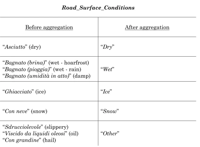
Finally, regarding the other attributes, in order to maintain a classification cri-terion that allows to compare these data with the UK data, some values have been aggregated and all the performed transformations are shown in the tables below.

Weather_Conditions

Before aggregation After aggregation

“Sereno” (sunny)

“Nuvoloso” (cloudy) “Fine” “Pioggia in atto” (raining)

“Grandine in atto” (hail) “Rain” “Nebbia” (fog)

“Foschia” (mist) “Fog”

“Nevicata in atto” (snowing) “Snow”

“Vento forte” (high wind)

“Sole radente” (slanting sunlight) “Other”

(41)

Road_Surface_Conditions

“Asciutto” (dry) “Dry” “Bagnato (brina)” (wet - hoarfrost)

“Bagnato (pioggia)” (wet - rain)

“Bagnato (umidità in atto)” (damp) “Wet” “Ghiacciato” (ice) “Ice”

“Con neve” (snow) “Snow” “Sdrucciolevole” (slippery)

“Viscido da liquidi oleosi” (oil)

“Con grandine” (hail) “Other”

Table 4 - AGGREGATIONS ON ROAD SURFACE CONDITIONS VALUES ABOUT ROME’S DATA

Light_Conditions

“Ore Diurne” (daylight) 2

“Sufficiente” (sufficient) 1

“Insufficiente” (insufficient)

“Inesistente” (no lighting) 0

(42)

3. PROBLEM ANALYSIS

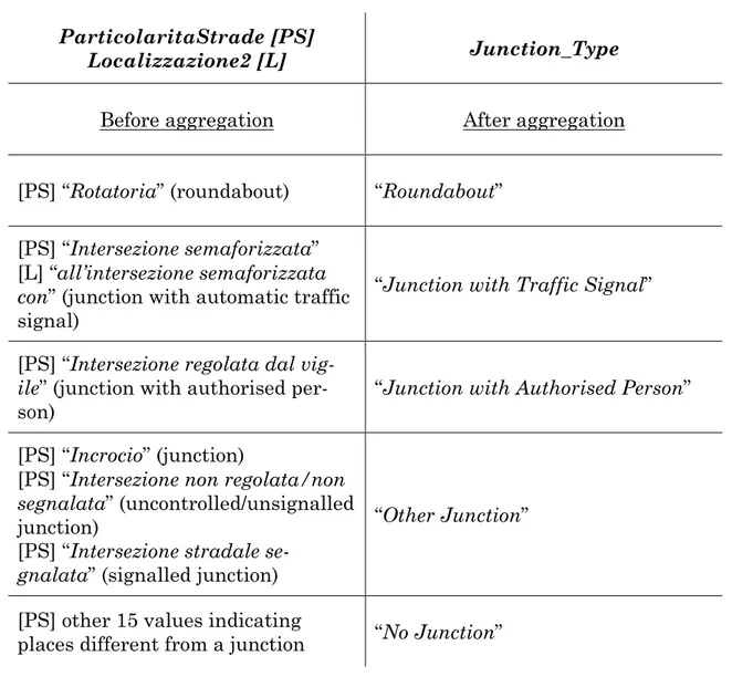
ParticolaritaStrade [PS]

Localizzazione2 [L] Junction_Type

[PS] “Rotatoria” (roundabout) “Roundabout” [PS] “Intersezione semaforizzata”

[L] “all’intersezione semaforizzata

con” (junction with automatic traffic

signal)

“Junction with Traffic Signal”

[PS] “Intersezione regolata dal

vig-ile” (junction with authorised

per-son) “Junction with Authorised Person” [PS] “Incrocio” (junction)

[PS] “Intersezione non regolata/non

segnalata” (uncontrolled/unsignalled

junction)

[PS] “Intersezione stradale

se-gnalata” (signalled junction)

“Other Junction”

[PS] other 15 values indicating

places different from a junction “No Junction”

Table 6 – AGGREGATIONS ON JUNCTION TYPE VALUES ABOUT ROME’S DATA

A clarification is needed about the last table, because getting exhaustive infor-mation about junction type is not so easy. “Junction with Traffic Signal” refers both to the value “Intersezione semaforizzata” of ParticolaritaStrade and to the value “all’intersezione semaforizzata con” of Localizzazione2. In this last case, simultaneously, ParticolaritaStrade always contains values indicating a junc-tion. These values, for all the other instances of Localizzazione2, correspond to different junction types.

(43)

At the end of the data pre-processing operations, 5,083 observations about young drivers are organized in a table having nine variables. Three of them are cate-gorical and they are Weather_Conditions (possible values: “Fine”, “Rain”, “Fog”, “Snow”, “Other”), Road_Surface_Conditions (“Dry”, “Wet”, “Ice”, “Snow”, “Other”) and Junction_Type (“Roundabout”, “Junction with Traffic Signal”, “Junction with Authorised Person”, “Other Junction”, “No Junction”). Five are ordinal and they are Hour (from “00” to “23”), Day_of_Week (from 1 [Monday] to

7 [Sunday]), Daily_Rainfall_Class (from 0 to 4), Light_Conditions (from 0 to 2)

and Estimated_Age (from 18 to 22). One is binary and its value depends on the gender of the driver.

3.3.2 Choice of the Number of Clusters

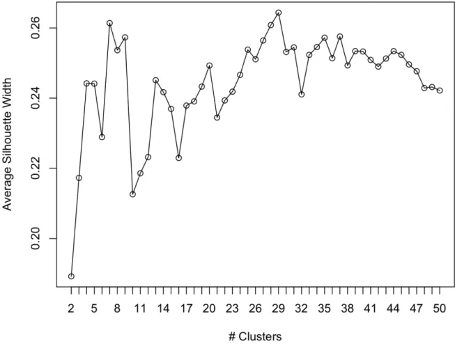
In R, the library cluster has a function, called daisy, that is used to compute the dissimilarity matrix between data objects. The table obtained at the end of the pre-processing phase has been given as input to this function and, as a result, a numeric value of the distance between each couple of observations has been ob-tained. In order to perform this calculation, the Gower’s coefficient has been used as the metric. According to this metric, the dissimilarity between two objects is achieved as the weighted mean of the contributions of each attribute. If a vari-able is categorical or binary, the distance between two values is 0 in the case of equal values and 1 otherwise. If a variable is ordinal, instead, the distance be-tween two values is the difference bebe-tween these values, divided by the total range. The function can also work with missing values and, if a variable contains a missing value, that variable is not considered in the distance computation. As is established practice, once the distance matrix is computed, the optimal number of clusters is found by trying to divide the data objects into k groups, for k comprised in a specific range, and choosing the value of k for which the simi-larity between objects of the same cluster and the dissimisimi-larity between objects

(44)

3. PROBLEM ANALYSIS

of different clusters is maximum. This operation has been performed making use of the PAM algorithm of the library cluster, with values of k ranging from 2 to 50. What has been obtained is shown in the following graph.

Figure 7 – AVERAGE SILHOUETTE WIDTH OF CLUSTERS IN ROME'S DATA

The average silhouette width is a measure of clustering validity, its value can range from -1 to 1 and a high value of average silhouette width means that there is a good similarity between objects belonging to the same cluster and a sub-stantial dissimilarity between objects of different clusters.

The highest value of average silhouette width is reached for k = 29, hence the characteristics of these 29 clusters have been investigated.

(45)

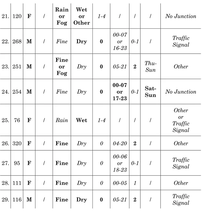
3.3.3 Characteristics of the Clusters

In the following table the features that characterize each cluster are illustrated. For each variable, the bold font indicates a characteristic that is common to all the observations of the cluster (or at most some missing values are present for that variable). On the contrary, if a feature is present in the vast majority of the elements of a group, but not in all of them, the italic font is used. A slash means that the variable is not relevant for the characterization of that cluster.

# of data ob jec ts gen der age w ea th er con di ti on s roa d su rfa ce con di ti on s daily ra in fa ll class hou r light c on di ti on s da y of w eek ju n ct ion type 1. 273 M / Fine Dry or Other 0 15-23 0-1 / Other or Roundabout

2. 162 F 19-22 Fine Dry 0 17-23 0-1 / Other or Roundabout

3. 171 M / Fine Dry 0 04-20 2 Mon-_Wed Other or Roundabout

4. 243 M 18-20 Fine or Fog

Dry or

Other 0 05-20 2 Mon- Fri No Junction

5. 205 M 21-22 Fine Dry 0 00-06 or 17-23 0-1 Mon- Fri No Junction 6. 81 M / Rain Wet 1-4 / / / Other or Traffic

(46)

3. PROBLEM ANALYSIS

7. 80 / / Fine Wet 0-2 00-06 or

16-23 0-1 /

Traffic Signal

8. 112 M / Rain Wet 1-4 04-20 2 / No Junction

9. 93 / / Fine Wet 0-3 / / / Other

10. 157 M / Rain Wet 1-4 00-06 or

16-23 0-1 / No Junction

11. 237 F 18-20 Fine Dry 0 05-21 2 / No Junction

12. 138 M / Fine or

Fog Wet 0-3

00-07 or

18-23 0-1 / No Junction

13. 110 F / Fine Wet 0-3 / / / No Junction

14. 113 F / Fine Dry 0 05-21 2 / Traffic Signal or Roundabout 15. 195 M 18-20 Fine Dry or Other 0 00-06 or

17-23 0-1 Mon-Fri No Junction

16. 222 M / Fine Dry 0 05-21 2 Sat-_Sun No Junction or Roundabout

17. 200 M / Fine Dry 0 00-06 0-1 / Other or Roundabout 18. 321 F / Fine Dry or Other 0 00-06 or 16-23 0-1 / No Junction

19. 258 / 21-22 Fine Dry 0 05-21 2 Mon-_Fri No Junction

(47)

3.3 Clustering on Rome’s Data 21. 120 F / Rain or Fog Wet or Other 1-4 / / / No Junction 22. 268 M / Fine Dry 0 00-07 or 16-23 0-1 / Traffic Signal 23. 251 M / Fine or

Fog Dry 0 05-21 2 Thu-Sun Other

24. 254 M / Fine Dry 0 00-07 or

17-23 0-1 Sat-Sun No Junction

25. 76 F / Rain Wet 1-4 / / /

Other or Traffic Signal

26. 320 F / Fine Dry 0 04-20 2 / Other

27. 95 F / Fine Dry 0 00-06 or

18-23 0-1 /

Traffic Signal

28. 111 F / Fine Dry 0 00-05 1 / Other

29. 116 M / Fine Dry 0 05-21 2 / Traffic _Signal

Table 7 – CLUSTERS IN ROME'S DATA

These clusters represent the most recurring types of car accidents in which young drivers have been involved in Rome. Their characteristics make them mutually exclusive. Observations having missing values are included in the clusters and, if the missing values are relating to variables not relevant for the characterization of the group, these data objects are even useful to determine the features of the cluster in which they are placed.

(48)

3. PROBLEM ANALYSIS

As a first consideration, the night hours in the weekend, which is the time period previously identified as the most dangerous, are a specific feature of the cluster 24, which, in addition, comprises only male drivers and mostly refers to acci-dents occurred in a place different from a junction. This could mean that young male drivers are more likely to take risks than females during these hours (high speed, drugs, alcohol) or, maybe, that young females don’t drive a lot at night in the weekend.

An other interesting aspect is that, except some rare cases, the age doesn’t rep-resent a discrimination criterion, therefore, it can be argued that there isn’t a big variation between the behaviours of the drivers in the age band of 18-22 years old.

The information about the total daily rainfall, instead, helps to distinguish be-tween accidents with various danger levels. In fact, wet road surface conditions with daily rainfall class 0, which means that the weather station did not register any rainfall, are present only in clusters having fine weather conditions and, therefore, a lower level of danger.

Regarding the most dangerous situation about weather and road surface condi-tions, male drivers are once again the most involved category, as they charac-terize three of the five considered clusters and, by summing up the number of observations inside these clusters, male drivers are about three-fifths of the to-tal number.

Fine weather conditions with dry road surface conditions are the most common combination of values about these variables, but this is probably due to the fact that, in Rome, the number of days in which it doesn’t rain in a year is much greater than the number of rainy days.

Finally, some values aren’t considered in the clusters, as they aren’t so frequent in the dataset. For instance, the value “Ice” about the road surface conditions is very rare and it can’t be used to characterize any group.

(49)

As a final remark, it’s worth specifying that the number of observations indi-cated in the second column of the table above is not the actual number of obser-vations having those characteristics. In fact, inside each cluster, there could be outliers (elements very different from the others), data objects wrongly assigned to that cluster and elements with a few different features. For this reason, after having identified the characteristics of each group, the elements not having en-tirely the features of any cluster have been counted and they are 178. Being 5083 the total number of observations, they only represent a small portion of data (3.50%) and some of them (11) also contain missing values.

(50)

4. METHODOLOGY

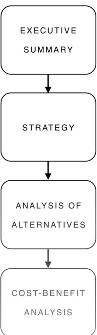
The aim of this work is to propose a business plan methodology modified to take advantage of the huge potentiality of open data and data science techniques. The four elements that a business plan can never lack are summarised in the following graph. Other parts, such as the description of the company and the development team, are not useful to deal with in this case.