POLITECNICO DI MILANO
Corso di Laurea Magistrale in Computer Science and Engineering Dipartimento di Elettronica, Informazione e Bioingegneria
Box Office Prediction and Transfer
Learning: a study on the US and
Swedish Market
Relatore: Prof. Paolo Cremonesi, PhD
Tesi di Laurea di: Alessandro Folloni, matricola 876311
Abstract
Motion picture industry has constantly growth in last decade. Still, this is a tricky business and box office failures could happen. Because of this, predicting the success of a movie, a task known as box office forecasting, is a problem worth studying. Forecast the success or flop of movies is a hard task, which involves the study of several variables, like cast, genre, MPAA, social network marketing, interest by the audience and so on. In many cases, such data is hard to collect, and, in many countries, there is a lack of data sources on movies.
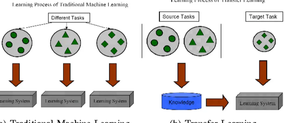
In this thesis we propose a new idea to solve the problem of scarcity of data in the field of Box Office forecasting. Traditional models use machine learning and statistical analysis to predict the gross of movies. Such studies usually analyze the US market as it is easier to collect data in a big market like America. In this study we propose to use transfer learning. The idea behind transfer learning is the following: use the knowledge from a source domain, which could be the US market, and transfer that knowledge to a target domain. Because of this, the research question that drives this study is the following: Can transfer learning improve the quality of predictions in a situation where few data is available? We focused our study on the Swedish market, which is an example of country where information is hard to find. We collected a data set of Wikipedia page views from the Swedish market and, using machine learning and statistical analysis, we developed a model able to forecast the box office premiere gross of a given movie.
We also collected the Wikipedia page views from the US market and applied transfer learning methodologies in order to improve the performance of Swedish models. In transfer learning terms, this means that the US is the source domain and Sweden the target domain. We finally compared the Swedish-only and Swedish-US models to see if transfer learning is beneficial or not.
Results show that the best performing model trained only on Swedish data is able to achieve a R2=0.83. The best performing model trained with transfer learning
and using both US and Swedish data achieve an R2=0.82.
The conclusion of this study is that transfer learning did not improve the performance in our context. These results are only related to this study. We believe that transfer learning was not beneficial to our study as the two studied markets, Sweden and US, behaves differently when it comes to movie selection.
Abstract
Nell’ ultimo decennio l’ industria del cinema è costantemente cresciuta, anche se flop cinematografici possono comunque avvenire. Per questo motivo sarebbe utile riuscire a predire il successo di un cinema. Prevedere il successo o fallimento è difficile e richiedo lo studio di molte variabili come il cast, il genere, i divieti, il marketing e l’ interesse dell’ audience di riferimento solo per citarne alcuni. In molti casi è difficile raccogliere queste informazioni e, in molti paesi, queste informazioni non sono nemmeno disponibili. Questa tesi propone un nuovo approccio per sopperire al problema della scarsità di dati disponibili nel dominio dei cinema. I modelli tradizionali usano tecniche di machine learning e analisi statistica per prevedere l’incasso al botteghino dei cinema. Questi studi utilizzano solitamente dati provenienti dal mercato americano poiché’ un grande mercato come l’ America offre una quantità maggiore di dati. In questa tesi proponiamo di usare tecniche di Transfer Learning per sopperire alla scarsità di dati. L’ idea alla base del transfer Learning è la seguente: usare la conoscenza disponibile in un dominio sorgente ( nel nostro case i dati raccolti dal mercato US) e trasferire la conoscenza implicita nei dati in dominio target. In questa tesina il mercato svedese è il dominio target in quanto esempio di paese dove è difficile raccogliere informazioni sui cinema. Abbiamo collezionato un data set che raccoglie, giorno per giorno, il numero di visite alla pagina Wikipedia di un film e poi abbiamo costruito un modello in grado di prevedere l’ incasso al botteghino di un singolo cinema. Inoltre abbiamo collezionato la stessa tipologia di dati per il mercato americano e applicato il Transfer Learning con l’ obbiettivo di migliorare le performance del modello svedese. Nelle conclusioni abbiamo confrontato le performance dei modelli predittivi allenati usando solo i dati svedesi e i modelli allenati usando dati sia US sia svedesi. Le performance raccolte mostrano che il miglior modello usa solo dati svedesi ed arriva ad una performance di R2=0.83, mentre il miglior modello allenato con transfer Learning arriva ad una performance di R2=0.82. Questi dati mostrano che il Transfer Learning non ha migliorato le performance del nostro modello, almeno nel nostro contesto.
Table of Contents Introduction 1 1.1 Background 1 1.2 Problem 3 1.3 Purpose 4 1.4 Goals 4 1.5 Methodology 4 1.6 Ethics and Sustainability 5 1.7 Delimitations 5 1.8 Outline 6 2 Extended Background 7 2.1 Box office forecasting literature review 7 2.2 Machine Learning required background 8 2.2.1 Generalization 10 2.2.2 Machine Learning nomenclature 11 2.2.3 Overfitting and underfitting 12 2.2.4 How to avoid overfitting and underfitting 15 2.2.5 Regression and classification 17 2.2.6 Linear, Ridge and Lasso Regression 18 2.3 Transfer Learning 20 2.3.1 Definition, notations and classification 22 2.3.2 Inductive transfer learning 23 2.3.3 Transductive transfer learning 24 2.4 TrAdaBoost for regression 25 2.4.1 TrAdaBoost idea 26 2.4.2 TrAdaBoost analysis 26 2.4.3 From classification to regression 29 2.4.4 Normalization 30 2.4.5 Output function 30 2.5 Other data analysis techniques 31 2.5.1 Data visualization 31 2.5.2 Correlation 33 2.5.3 Regression metrics 35 3 Methodology 41 3.1 Problem understanding 41 3.1.1 Box Office forecasting literature review 41
3.1.2 Problem definition 42 3.1.3 Transfer Learning literature review 42 3.2 Model Selection 43 3.2.1 Model selection for Box Office Forecasting 43 3.2.2 Selection of transfer models 44 3.3 Model Performance 45 3.4 Data source selection 45 3.4.1 Data format 47 3.5 Evaluation 47 3.6 Validity threats 48 4 Results 51 4.1 Data Set Analysis 51 4.2 Raw Predictions 53 4.3 Feature Selection 54 4.3.1 Feature selection on US data set 56 4.4 Transfer Learning aided training 57 4.5 Discussion 58 5 Concluding Remarks 61 5.1 Contributions 61 5.2 Validity of our study 61 5.3 Discussion on goal achievements 62 5.4 Future Work 62 Bibliography 63
Introduction
Box Office forecasting deals with the problem of forecasting the financial success of movies before the movie goes into screening rooms. A model that correctly forecast movie success would help the entire motion picture industry by enabling informed investment decisions, improving marketing decision and entry time strategies.
Accurate forecast in early stage is a tough challenge. There are many factors that contributes to the success, or failure, of a movie. That information is not available in the early stage of production. For example, a factor that greatly impacts the success or failure of a movie is the public chattering that the movie generates. Apart from exogenous factors, a movie is an experience product, strictly connected to the taste of the audience and not related to evidence. Because of this, it is extremely hard to know whether the audience like, or dislike, a movie before watching it.
In recent years box office forecasting has been studied and recent approaches focus on developing forecasting models based on Machine Learning.
1.1 Background
In the last decade Machine Learning has made a large impact in several fields, from academia to every-day life. Many applications, tools and services that are nowadays common use machine learning under the hood. Netflix, for example, is a web streaming platform. For a small monthly fee, Netflix’s users get access to video content, movies and web-series. How machine learning fits in this? Netflix is able to recommend, with some margin of error, which user would like a certain content, and thus is able to recommend that content to the user. Another example are virtual assistants and bots. Siri from Apple, Alexa from Amazon and Cortana from Microsoft, these are virtual assistant that are nowadays living in our homes. You can ask Siri to call and set timers for you as if you are talking to someone, despite the fact that there is an algorithm behind. Or ask Alexa to manage the temperature of your flat. These are only a couple of examples. Underneath, there is Machine Learning, a field of study that lies between computer science and mathematics. At his core, machine learning is a set of techniques that leverages statistical methods in order to continuously improve the performance on a specific task.
Machine Learning is a big word, sometimes abused. By itself, Machine Learning is a word that groups together different types of algorithms. According to [1],
there are different branches of Machine Learning: • Supervised Learning;
• Unsupervised Learning; • Semi-supervised learning; • Reinforcement learning
Other branches and other classification exist, however these are the most known branches of ML.
The common point of all Machine Learning techniques is data. Machine Learning cannot work and is useless without data. The success of Machine Learning can be explained by the fact that we live in the Big Data society. We produce an immense amount of data without even knowing it. Every action we do on Facebook, our photo on Instagram, our search interest on Google and items we buy on Amazon. Every action is logged and used by automatic algorithms. And this is only the human-generated data, because we do not consider the data generated by sensors and autonomous agents like chips, cars and so on. With the increasing amount of data, human analysis is not anymore feasible, and thus Machine Learning gained success.
Despite this enormous amount of data, there are still situations where data is not highly available. The reason of this are different and specific for each domain. In many situations the data is never collected, or even if collected, it might be that collection still happens on paper and not in digital format. Many data sources are proprietary: data is collected, but it is not available to a public audience. An example of this is military data. Or you just need to pay a fee, like with financial historical data. In other situations, data is available and in a digital format, but it is unlabeled, meaning that someone need to label it in order to make that data useful. In recent years, for example, machine learning has been applied to medical images with the aim of detecting illness( [2] [3] [4] [5] [6]). Medical images are available in a digital format, but in most scenarios, it is not enough to
school we learn the numbers, then we learn calculus. As we go on we use prior knowledge to learn new concepts. In transfer learning terms, we transfer our knowledge to a new domain or a new task.
Another domain where we find scarcity of data is movie market. In particular, data regarding movies that are, or were, in the movie theaters is hard to find. Actors, director, genre, ratings etc. are rather easy to find for famous and budget-heavy movies, however other factors like financial success, or failure, and the impact of a movie on social media platforms is much harder. Moreover, data is much easier to find provided that the movie has been produced in US. For other movies, like local movies or non-English movies, is way harder to find. There are also situations where data sources are available only in some countries. US is the biggest player in the motion picture industry, and thus data is generally easier to find compared to other smaller countries, like Sweden.
1.2 Problem
Literature review, which is available in Section 2.1, shows that Box Office Forecasting is a topic in which both academy and industry are interested. There has been research in explaining which variables is more predictive in terms of box office success or failures, which model better explain consumer behavior, whether it is possible to know in early-stage production the outcome of the movie. All methodologies employed, mostly linear regression, statistical modeling and Artificial Neural Network, share a common point: they use data from previous movies. The core of these analysis, no matter the approach is data. Some studies reported the number of samples used in their analysis. Between these studies, most of them use a small sample of movies.
It is clear that, in order to increase reliability of these studies, more data is required. There could be several reasons why data is hard to find, for example data is not available, cannot be collected, it takes too much effort to collect, it is privately held, etc.
The problem found in this area, which is the focus of this thesis, is the scarcity of data.
Most of studies focus their attention on the US market, which is the biggest and, in movie production, the most flourishing. Because of this, it is easier to find data in this market. What about smaller countries? What if someone needs to study small market?
1.3 Purpose
The purpose of this thesis is to propose and analyze a new methodology for dealing with the scarcity of data in the field of box office forecasting. In particular, in this work we propose to use transfer learning.
Transfer learning is presented in Section 2.3.3. However, to give the reader an idea, we give an overview of transfer learning here. The idea behind transfer learning is the following: use the knowledge, if any, from a source domain and transfer that knowledge to a target domain. That knowledge may, or may not, improve the quality of predictions in the target domain.
In this thesis we study box office forecasting in the US and Swedish movie market. Following the previous idea of transfer learning, the US market is the source domain, and the Swedish market the target domain. We aim at studying the box office gross in the Swedish market using the data from US and Sweden. This idea in not US or Sweden specific, and can be applied to any other markets as well.
Because all types of research should be driven by a clear research question, considering the problem of scarcity of data and the related purpose, we specify the following research question:
Can transfer learning improve the quality of predictions in a situation where few data is available?
1.4 Goals
This thesis has a short-term and long-term goal. The short-term goal is to build a model for box office forecasting specifically designed for the Swedish market. The long-term goal is to illustrate a novel idea in the field of box office forecasting and thus, provide the basis for further research in the field.
both the field of Box Office Forecasting and in the field of Transfer Learning. This phase aim is to get familiar with the area, terminology, variables and algorithms used in box office forecasting.
Following literature review, the focus moved on (i)model selection, (ii)model performance assessment and (iii) data source selection. Between the models proposed, linear regression was chosen for simplicity and performance/training-time tradeoff. Following this decision, and due to the nature of the problem, we decided to evaluate the performances of models using R2 coefficient. Concerning
the data selection, we decided to use Wikipedia page views as features and box office premiere gross as target.
Because there is no theoretical framework to address whether the transfer of knowledge happened or not, and because there is no way to know if transfer learning is beneficial prior to experiments, we based our conclusions using comparison. We trained several models, some with the employment of transfer learning, some without transfer learning. We then collected performance metric and compared performance between each other. Since the only difference is the usage of transfer learning, if transfer learning helps the model performance, this is reflected by having a better performance.
1.6 Ethics and Sustainability
Box office forecasting is a task bounded with sustainability. A model that correctly predict gross is, with a certain degree, able to understand the number of customers. Knowing the number of customers is very helpful: for example, when a small batch of customers is forecasted, projection rooms can be closed saving electricity, air conditioning and human labor.
1.7 Delimitations
This project looks to a particular snapshot of the problem. We considered only machine learning and linear regression as algorithms for box office forecasting. Also, we looked at a specific time-frame: we only focus our prediction model to forecast the gross of movies during the premiere week-end (the first week-end the movie is out in the screening rooms) and we did not study the drop-off effect which follows premiere. This can be seen as a limitation, however the reason of that choice is explained in Section 3.6.
1.8 Outline
The remainder of this document is organized as follows:
Extended Background extended the background section previously presented. In
the extended background we present the concepts required to understand the reminder of the work.
Methodologies describes the steps and decisions made during the development of
this project.
Result section presents the results of the research and discus them.
Final Remarks conclude the work by answering the research question and
2 Extended Background
This chapter presents the concepts and necessary theory upon which the thesis has been built. The aim of this chapter is thus not to present to the reader a full resume of machine learning, but only provide the concepts and theory necessary to the comprehension of later chapters. In case the reader is interested, a good book on Machine Learning, well known to machine learning practitioner, is the Bishop [7].
The following chapters are organized as follows:
Box office forecasting literature review presents the literature related to Box
Office Forecasting.
Machine Learning required background contains the machine learning (and
statistical modeling) concepts required to understand this thesis. Machine Learning and statistical modeling are presented together as statistics and Machine Learning most of times works together.
Transfer Learning contains the concepts and algorithms employed in this
project. Since transfer learning is not well known, we present transfer learning in a different chapter with respect to machine learning.
TrAdaBoost for regression presents the detail of TrAdaBoost algorithms, for this
thesis adapted to a regression problem. TrAdaBoost is transfer learning algorithms, however it requires a special presentation as it is rather complex compared to the other algorithms.
Other data analysis techniques present different techniques that are employed in
this thesis. In particular, we discuss about data visualization, correlation and evaluation metrics.
2.1 Box office forecasting literature review
Box Office Forecasting is a problem that already gained interest. In 2007, a group of researchers tried to build a model with natural language processing, which is a branch of machine learning, in order to evaluate scripts that will lead to more profitable movies [8].
Watching a movie is an experience. As so, the enjoyment of a movie is strictly related to the mood of the audience. It is therefore important to measure the mood of the consumers. A framework for the study of consumer behavior with statistical modeling has been proposed [9] [10].
[11] is possibly the first work in the field of econometric analysis of motion pictures. It used MPAA ratings, stars, cost and distributors as input variables and fitted a linear regression model. Following this line of inquiry, [12] and [13] used linear regression as well, but on a different set of input variables. Latter studies reported a predictive performance slightly better than [11]. [14] built a different linear regression model using movie characteristic as before plus Word of Mouth1
(WOM) information. [14] obtained a rather good performance, even if they studied a smaller time-frame compared to previous work.
Other streams of research which does not employ linear regression models, exist. BOXMOD-I [15] model leverages queue theory and statistics and MOVIEMOD [16] goes in the same direction, adding WOM variables to the previous model. [17] [18] used diffusion based model, which studies the spread pattern of a new product and/or service in a social system by determining how it is perceived by customers.
Recent studies feature advanced machine learning, like Artificial Neural Network (ANN) and decision trees. [19] classify movies into 9 bins, from ‘flop’ to ‘blockbuster’ leveraging classical movie characteristics. [20] used a similar technique, with the use of an ANN and the aim to classify the movie into six possible bins, ranging from ‘blob’ to ‘bomb’. [21] used a particular neural network, known as Bayesian belief network, to investigate the casual relationship among movie features in the performance prediction of box office success. Following that, they searched which features is related to box office bomb. [22] used the blogosphere and proposed eight different machine learning models to forecast sales. [23], in a recent work, studied the Korean movie market, employing traditional features and WOM effects. They used genetic algorithms to evaluate features importance and then fitted a forecasting model. In an earlier work [24] they developed tree different and sequential models which work (1) prior to, (2) a week after and (3) two weeks after release.
Machine Learning is today almost half-a-century old, but it is only in the last decade that it has become a phenomenon. The term “Machine Learning” was coined by Arthur Lee Samuel in 1959 [27]. According to his definition, ML is
The field of study that gives computers the ability to learn without being explicitly programmed to do so
However, the field of learning programs had started some years before 1959. The famous Alan Touring, the genius behind Enigma, who helped the British
government win the World War II by decrypting Nazis telecommunication
system, invented the so called “Touring Test”. In this test, a computer has to fool a human to prove the computer is able to think. If the computer passes this test, he has “real intelligence”. Frank Rosenblatt [28], in 1957, invented the
perceptron. The New York Times and later The New Yorker billed his work as revolutionary 23. The perceptron was the first supervised learning algorithm for
binary classification. Although being a simple linear classifier, perceptron set the ground for later research and in 1974, Werbos [29] invented backpropagation. With these tools, and an advancement in computer computing power, today Deep Learning is now possible.
Tom Mitchell [30] proposed a definition of Machine Learning, more rigorous compared to the former.
A computer program is said to learn from experience E, with respect to tasks T and performance measure P, if its performance on T as measured by P
improves with experience E.
From Mitchell’s and Samuel’s definitions, it is clear that Machine Learning uses a different paradigm compared to typical programming paradigm. Traditional programming, also called imperative programming, processes input data and returns to user an output. The output depends on the input, the mapping
function between input/output is the program. Machine Learning, instead, uses the input and output and (tries to) learn the mapping function. The mapping function can then be used to predict the output on unseen input. These concepts are shown in Figure 1.
2 https://www.nytimes.com/1958/07/08/archives/new-navy-device-learns-by-doing-psychologist-shows-embryo-of.html
Figure 1: Tradition Programming vs Machine Learning
To sum up, Machine Learning is not intended to solve a specific task, but rather to learn a task by continuously improving from past errors.
The reminder of this presentation on Machine Learning is intended for the Supervised learning setting. Supervised Learning, according to [1], deals with labeled data. The objective of a learner algorithm is to find a relation, a model, which identifies a relationship between the data instance and the corresponding label.
2.2.1 Generalization
Machine Learning is, in his nature, inductive. Starting from the data, which are observations from the real word, ML aims at extracting a model which (should) represent reality. In other word, starting from a set of observations, ML aims at obtaining the general model. This ability is called generalization. If the model generalizes well, that model can be applied to new input data and the model returns the correct output. If the model does not generalize, then, when that
case, each student is like a Machine Learning algorithm. Students are not programmed to solve calculus operation, but the teacher shows them equations (the input), how to solve them, and the result (the output). Students, by training, learn how to solve equations, therefore they learn the model which binds input and output. During the test, the teacher submits to them new equations and, if the students have learned the right mapping, they should be able to provide the output.
2.2.2 Machine Learning nomenclature
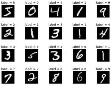
Machine Learning uses daily-used words, like features or examples, with a specific meaning. Here we provide the basic nomenclature. To match the concepts with examples we use the famous MNIST data set & challenge. The MNIST challenge aim is to recognize handwritten digits. The digits are provided as a 28x28 pixel image, which can be represented as a vector x of 28x28=748 real valued elements. These elements are called features. The goal is to produce a model that is able to match the input vector x with the right output digit. An example of the input image/label is provided in Figure 2.
Figure 2: MNIST input picture and label example
Using machine learning for this kind of task, we would use a large set of N digits {x1, x2, …, xN} in order to tune an adaptive model. The N digit set is called
training set. Each digit in the training set has a label attached to it. The label is
the output value, what the model should output after having seen the corresponding input image. The set of labels is also known as target or label
vector t = {t1, t2, …, tN}. The result of running a machine learning algorithm is a
program (see Figure 1). We will use the term program, model or mapping
function interchangeably. In mathematical terms, the program is a function y(x)
which takes as input xi and return the output ti. The function y(x) is an adaptive
function, meaning that the form of the model has to be learnt during the training
phase. During this phase, the machine learning algorithm scans one or more time
the training data set with the aim of learning the mapping function. Using the student example, training is the time dedicated to studying and homework. Once the training has completed, the model y(x) can be used to infer the label of new unseen pictures. This phase when the model has to infer on new examples is called test phase or test time prediction. Following from the previous chapter, the ability to categorize correctly new examples different from those used during training is called generalization.
2.2.3 Overfitting and underfitting
When a model does not generalize, there are two possible scenarios: overfitting and underfitting. To illustrate those concepts we use another example, the polynomial curve fitting. The images and documentations of this experiment is taken from the Bishop [7]. The data of this experiment is generated from the function sin(2&') adding random noise. The training set is composed by N observation of x, x = {x1, x2, …, xN} and the labels t = {t1, t2, …, tN}. Figure 3 shows
the plot of the training data set. The blue dots represent the training examples, the green line is the real function sin(2&'). {x1, x2, …, xN} were chosen by
uniformly sampling in the range [0,1], while the label has been generated using the formula () = sin(2&')) + ., where . is random noise. The model should learn the function y(x) = sin(2&').
Figure 3: Plot of the training data set, with N=10
A simple model would be a polynomial function 1(', 3) = 45+ 46' + 47'7+ ⋯ + 4
9'9 = : 4;'; 9
;<5
Where M is the order of the polynomial, xj denotes x to the power of j and w =
{w0, …, wM}. w is the vector of coefficients and those are the adaptive part of the
model. In fact, those values have to be learnt during the training phase. So, how are the vector of coefficients learnt? Before answering to this question, we have to define the model error. This imply that we have to define an error function that measures the error between the model y(x,w) and the training data point. A common error function, widely used, is the sum of squares of the error, also known as Residual Sum of Squares (RSS). RSS is defined as
=>>(3) = 12 :{1('A, 3) − (A}7 D
A<6
The 1 2E is included due to mathematical reasons. We should note that RSS is non negative quantity that can only be 0 if, and only if, the model y(x,w) can correctly predict the target for all input xi – output ti. The above formula defines the error
over the training data set for all possible set of w. We should choose the model that have the smallest possible error, therefore the smallest RSS. Because the error function is a quadratic function of the coefficients w, its derivatives with respect to the coefficients will be linear in the elements of w, and so the minimization of the error function has a unique solution, denoted by w*, which
can be found in closed form. The resulting polynomial is given by the function y(x, w*).
We now know how to choose the right set of coefficients w, yet we do not know how many coefficients, the parameter M. The problem of choosing the right M is known as model selection or model comparison. Figure 4 shows four different models with M=0,1,3,9. The red line represents the model after it has been trained. Models with M=0 and M=1 give poor fits to the data. This results in a poor representation of the function sin(2&') and a high RSS. Model with M=3 seems to offer the best approximation of the real function sin(2&'). Model with M=9 offers an excellent fit to the training data because it interpolates all the training points. Because of this the error RSS is 0. However, the plot shows that the model M=9 offers a bad representation of the original function sin(2&') and the generalization is not good. This latter behavior is known as overfitting. In general, overfitting is the situation where the error (in this case measured with RSS) evaluated over the training data set is small, but the error function evaluated over non-training samples is high. On the other hand, the models with M=0 and M=1 are two examples of underfitting. The model has not enough parameters to correctly represent the original function sin(2&'). If the reader thinks at it, model M=0 corresponds to the model 1(', 3) = 45. This model is
only able to learn a line that is parallel to the x axis. Model M=1 is the model 1(', 3) = 45+ 46' which is only able to learn a straight line. Neither of the two models are able to learn an oscillating function such as the sin.
Figure 4: Plots of polynomials with different degrees
2.2.4 How to avoid overfitting and underfitting
In previous section we explained overfitting and underfitting. The two of them are possibly the most important errors that can happen in data science. So, we need a way to detect underfitting and overfitting. We shall recall the general idea of overfitting and underfitting: the former is the situation when the model scores good on training data, but perform bad on unseen data, the latter is the situation when the model has not enough “power” to represent mapping function, therefore the score on both training set and unseen data is bad. In general, to detect fitting problems, we need at least 2 sets: the training set and the test set. Both training and test sets must have the same structure and must be observation of the same phenomena. To give the reader an example we use the previous examples on MNIST data set. Using MNIST data, we can split the original data set in 2 sub-set: 75% of the images-labels are used for training purpose, the remaining 25% for testing purpose. In this way, the training phase will see only part of the data set. At test time, we use the remaining 25%. This technique of
splitting the original 100% data set is very well known in machine learning and data science field and it is known as train-test-split. Common values for train-test set split are 75%-25%, 80%-20%, 90%-10%. If the reader thinks about it, this is the same situation as the student example mentioned earlier. The professor usually takes the exercises from a book: most of the exercise are used for train the student, the others for testing them.
Train-test split is possibly the easiest and most known form of obtaining a train and test set from a data set. Other methodologies, more complicated, exist. In this thesis we will use k-fold cross validation and leave-one-out cross validation. In cross validation the original data set is divided into k non-overlapping sub- sets; usually k is 5 or 10. In each experiment 1 subset, also called fold, is used for testing and the remaining folds are used for training. Figure 5 illustrates cross validation. The final results are k models with k performances, usually the average of the k models is the final results. Leave-one-out cross validation follows the same concept of k-fold, with k equal to the number of examples in the original data set.
Figure 5: k-fold cross validation, with k = 5
In Machine Learning literature, train-test-split and cross validation falls under the name of model selection.
Figure 6: Train and test errors against model complexity.
As the reader may notice, when the model complexity (e.g. the degree of polynomial M) plays an important role. Reading the plot from left to right, the reader may notice that train and test errors decrease together. We already know that for M less than or equal to 3 we have underfitting. And the plot shows that: in fact, by giving the model more “power”, the error decreases. Recall that underfitting is the situation with a high train and test error. With M between 3 and 8 the error is more or less stable and most important, the lowest on the plot for both train and test sets. We already know that those are the models we are looking for as are those with the lowest error. With M=9 the 2 errors diverge: this is overfitting. It means that the model fitted only the training data (in fact the train error is almost 0) but did not generalize well on test data (in fact the test error rocketed).
2.2.5 Regression and classification
In previous chapters we saw two different supervised learning examples, the first is the MNIST data set and the second is the polynomial curve fitting. These two examples are example of classification and regression problems, respectively. In classification the number of possible labels is known and countable. The algorithm must return as output a category between the ones seen during training.
The polynomial curve fitting is an example of regression because the target label is continuous and infinite. Because of its infinite nature, not all possible labels can be seen during training, therefore the algorithm must be able to calculate the output.
This difference is rather import because it drives which algorithms can be used. In the broad field of supervised learning, there are algorithms for regression and algorithms for classification. Some of them can be used for both task, some are mainly for classification and other for regression only.
In this thesis we deal with a regression problem as we try to predict the gross, in American dollars, of movie box office.
2.2.6 Linear, Ridge and Lasso Regression
Linear regression is possibly the simplest statistical techniques for predictive modelling. It models the relationship between the target (dependent variable) and features (or independent variables). The relationship between the target and features is modeled in a linear fashion. The unknown parameters of the function are estimated from the (training) data. The general formula of linear regression is the following:
1(G, 3) = 45+ 46'6+ … + 4I'I = : 4;';
I
{;<5}
This formula is very similar to the one used in polynomial curve fitting example, however in this case we do not use the power-of operator. In this formula the array w = {w0, w1, …, wD} is the parameter or coefficient vector and, as in the
previous example, it is the set to parameters that has to be found. The array x = {x1,…,xD} is the features or independent variables array. The prediction of the
linear model is the linear combination of independent variables with the coefficients. The first coefficient, w , has a special name and is called the bias.
difference between the prediction made by the model 1(GK, 3), and the real value the model should predict ti. This difference is evaluated over all training
examples (we assume N examples in the training set). This is Linear Regression. Empirical evidence shows that vanilla Linear Regression does not work well when the number of features is high. Coefficients tends to assume large absolute values. This is an example of overfitting. In such scenarios, a technique that is often used is regularization. Regularization means to add a penalty term to the error function in order to discourage coefficients from reaching high values.
Ridge regression uses the same model but adds the L2 regularization to the error
function. The error becomes
J(3) = :{1(GK, 3) − ()} + L 2M|3|M 7 D )<5 Where ||w||2 = wTw = 4
57+ 467+ ⋯ + 497 and the coefficient λ governs the
relative importance of the regularization term compared with the sum-of-squares error term. In statistics literature L2 regularization is known as shrinkage as it
shrinks the absolute value of the coefficients. Ridge regression is also known as
weight decay.
Lasso regression follows exactly the same idea of Ridge regression but adds the L1
regularization factor to the error formula. The result is J(3) = :{1(GK, 3) − ()} + L
2M|3|M
D
)<5
Where ||w|| = 45+ 46+ ⋯ + 49.
Despite being very similar in shape, Ridge and Lasso have a different mathematical background and, thus, different properties. A full review and explanation of those is out of the scope of this document. The reader may refer to [7], Chapter 3.
In this section we introduced the basics of Machine Learning. Linear, Ridge and Lasso regression, which we refer to as Linear models, are the models that will be employed in order to make the predictions on the box office gross. As a matter of fact, the gross is just a number and will be the target of our linear model. The features, or dependent variables, are introduced in the Methodology section.
Linear models assume all observations have the same importance. In order to inject new knowledge, and evaluate the importance of each sample, we need to use Transfer Learning.
2.3 Transfer Learning
In the previous section we have introduced the basic concepts regarding Machine Learning. However, many of those algorithms works well under a common assumption: the training and test data came from (i)the same feature space and from (ii)the same distribution. This statement may seem a little abstract, so we now try to clarify it. The (i) point say that train and test data must have the same structure. That is to say, if the train features are, for example, 100, also the test features must be 100. If the feature 9th in training data set is a categorical
variable, this must be the same in the test set. Structure of train and test set must be equal. Point (ii) say that training and test data must be from the same distribution. This concept comes from statistic. Machine Learning assumes from a statistical perspective that the examples in train or test set are observation of a random process. In such way, the examples are observations drawn from a random variable. Machine Learning aims at understanding the model (recall Figure 1) behind, thus understanding the random process that generate the observations.
When the assumption(i) and (ii) are not met, traditional Machine Learning fails. In such scenarios, models need to be rebuilt from scratch using new data. Collecting new data is, in some case, impossible or, more frequently, expensive, so it would be nice to reduce the need and effort required to collect new data. Instead of collecting new data, we may use other data set or other models that have been used in close related situation, and then transfer the knowledge between the task or domain closely related to our requirements. [2] [3] [4] [5] [6] did that in the field of medical images. They used models, in particular Deep
with Deep Learning. In the very first lesson, he is already using transfer learning for image recognition. In this context, transfer learning has been used to speed up the training process. The teacher uses it in order to fine tune a model already trained for image recognition and adapt it to work on a specific data set. This is exactly the same method applied for medical image analysis.
Transfer Learning is helpful in other domains not related to Deep Learning. For example, Web-document classification [31] [32] [33] deals with the problem of classifying web documents into several predefined categories. Say that we have the web pages of different universities and these pages have already been labeled with the target we are interested in. Labeling of those pages took time. On that data, we built a model for classify university pages. We now want to classify the web page of a company, for which we do not know the label. We cannot apply the previous model as the model expect a university web page, not the web page of a company. It would be nice to transfer the classification capability of the previous model instead of creating a new data set for companies.
Also, transfer learning can be helpful when data can be easily outdated. In such case, the labeled data can change distribution over time and recent collected data might follow a different distribution with respect to old data.
Lastly, transfer learning has proven helpful in language study. A model trained for a language can be adapted to work on a different language [34].
To sum up, transfer learning is beneficial for mainly two reason. First, it can be used to speed up the training process, which in modern deep learning models takes long time. Second, when we do not have enough data in a domain, we can use data in a different, but similar, domain. A model which is first trained on this second domain can be adapted, or re-trained, in order to work on our original domain. The general idea of transfer learning is shown in Figure 7.
Transfer Learning has been studied for (mainly) supervised, unsupervised [35] [36] and reinforcement [37] [38] learning. Since in this thesis we deal with supervised learning, we present only transfer learning for the supervised setting. In this chapter we present transfer learning. In Methodology section we present which algorithms has been implemented and tested for this study and why those algorithms have been chosen.
2.3.1 Definition, notations and classification
Before defining what is Transfer learning we should introduce and define the concepts of domain and task. These are the two pillars upon which transfer learning relies.
Definition: Domain A domain D consists of 2 components: a feature space χ and a marginal probability distribution P(X), where X = {f1, ..., fn} ∈ χ
On the basis of Domain D = {χ, P (X)} concept, a task is
Definition: Task A task consist of 2 components: a label space Υ and an objective predictive functions f(.) which is not observed but can be learned from the training data, which consist of pairs {xi, yi}, with xi ∈ X and yi ∈ Υ. The task is denoted by T = {Υ, f(.)}
Notation slightly changed from the previous sections. Here the model mathematical function is called f(.), whilst in previous section was y(x, t). As well, the target is here called y instead of t. This change of notation has been done for 2
The simplest and most studied case of transfer learning involves two different domains: a source domain DS and a target domain DT. Usually transfer learning
assumes that 0 < nT ≪ nS, where nS is the number of instances in DS and nT is the
number of instances in DT.
We are now ready to define what transfer learning is.
Definition: Transfer Learning Given a source domain DS and a learning
task TS, a target domain DT and a learning task TT, transfer learning aims to help improve the learning of the target predictive function fT (.) in DT using the knowledge in DS and TS, where DS ≠ DT or TS ≠ TT.
The condition DS ≠ DT implies the either χS ≠ χT or PS(X) ≠ PT(X). Recalling the
example on web document classification, the source and target domains have different language (χS ≠ χT) or source and target deal with different topics (PS(X)
≠ PT(X)).
At the same way the condition TS ≠TT implies that either ΥS ≠ΥT or P(YS|XS) ≠
P(YT|XT). In the document classification example, the case ΥS ≠ΥT happened
when, for example, the source domain has binary target and the target domain has 10 classes to classify the documents to. The second case, P(YS|XS) ≠P(YT|XT),
corresponds to the situation where source and target documents are unbalanced in terms of user defined class.
When TS =TT and DS = DT the learning process becomes a traditional machine
learning problem.
Transfer Learning can be classified according to what we have already seen. When TS ≠TT we are dealing with inductive transfer learning, not matter when
the source and target domains are the same or not. In trasductive transfer
learning the source and target tasks are the same and source and target domains
are different. In particular, the situation where the feature space between domains is the same, RS = RT, but the marginal probability distribution of input
data is different, P(XS) ≠P(XT), is called domain adaptation. 2.3.2 Inductive transfer learning
According to [39], the definition of inductive transfer learning is the following.
Definition: Inductive transfer learning Given a source domain DS and a
learning aims to help improve the learning of the target predictive function fT (.) in DT using the knowledge in DS and TS, where TS ≠ TT.
Inductive transfer learning requires a few labeled data points in the target domain in order to induce the target predictive function.
Instance-based transfer approach groups together the methods that tries to
reuse the instances of the source data set. TrAdaBoost [40] leverages boosting, in particular the original AdaBoost. It assumes that source and target domains use exactly the same set of features and labels, but the distribution of the data in the two domains are different. TrAdaBoost will be explained in detail in the next section.
Other approaches in this area have been proposed. [41] proposed a method to remove training example from source domain that are too different compared to the target data set. The difference is evaluated over the conditional probabilities (YS|XS) and P(YT|XT). [42] proposed a methodology to label data in the target
domain with the help of source data. [43] focus the attention on classification problem using the Support Vector Machine algorithm.
Other methods and approaches exist in inductive learning, however they use rather advanced methodologies which are not studied in this work.
2.3.3 Transductive transfer learning
According to [39], the definition of inductive transfer learning is the following
Definition: Transductive transfer learning Given a source domain DS and
a learning task TS, a target domain DT and a learning task TT, transductive transfer learning aims to help improve the learning of the target predictive function fT(.) in DT using the knowledge in DS and TS, where DS ≠ DS and TS =TT
• The SrcOnly model ignores the target data and trains a single model using only the source data;
• The All model trains a standard learning algorithm on the union of the two data sets;
• The Weighted model assigns a weight to each instance. Instances from the Target domain usually get a weight of 1, while instances from the source distribution get a weight lower than 1. Weights are chosen by cross-validation. The weighted approach solves the problem that, when source instances are way more than the target instances, source instances can wash out the target instances;
• The Pred model uses the output of a model trained on Source instances as a feature. First, we train a SrcOnly regressor, then we run the SrcOnly model on the Target data set. The predictions are used as an additional feature on a second model trained over the target augmented with this new feature;
• The LinInt model linearly interpolate the predictions of the SrcOnly and the TgtOnly models. Interpolation ratio is adjusted based of training sample.
[46] proposed a model to beat previous baseline models, however its efficiency is not always assured. [47] proposed a model that constantly outperform the previous baselines [45], however its implementation is far more complicated and training times is 10 to 15 times longer.
In the field of transductive transfer learning other research exist, for example the sample selection bias problem [48]. Those however are not useful for our domain and are not studied further.
We postpone the selection of adopted algorithms to Methodology section.
2.4 TrAdaBoost for regression
In this section we present the TrAdaBoost algorithm. TrAdaBoost is an inductive transfer learning methodology which works by reweighting the instances of source and target data sets. TrAdaBoost is a difficult and hard to understand algorithm, so it this section is dedicated to the explanation of it. As the reader may guess, in this thesis we implemented it, however not in its original formulation. In his original paper [40], TrAdaBoost was first developed for binary classification. Since we are dealing with a regression problem, we adapted
TrAdaBoost to work on regression task. After the implementation and testing, we found out that this adaptation was already studied [44], even if not implemented. TrAdaBoost is base algorithm over which more advanced method works, like [45] [46].
2.4.1 TrAdaBoost idea
TrAdaBoost uses the idea of boosting, developed in the 90s, and applies it to transfer learning field. The math behind boosting is rather harsh and long, therefore we explain here the intuition behind boosting and we later on focus on just TrAdaBoost. The reader interested in the mathematical foundation of boosting may refer to [47] and [48].
The idea of boosting is to sequentially train a series of models in such a way that each following model focus on the error of the preceding model. We now propose an example taken from the Data Mining lectures of prof. Luca Lanzi, Politecnico di Milano.
A patient suffers of headache, stomachache and back-pain. He goes to doctor 1, doctor 1 explain and solves stomachache. After, he goes to doctor 2, which solves the back-pain problem. He then goes to doctor 3, which solves headache. This the idea: each doctor solves one problem. The following doctor solves the problems which the previous ones do not address. In practice boosting assigns a weight to each sample in the data set, each weight represents the importance of the assigned sample in the data set. During learning, each model focuses in giving better predictions to samples with a high weight. Weights are adjusted at each step during the learning process in such a way that following models focus on samples that the previous model is not able to predict correctly.
The key idea of TrAdaBoost is to use boosting to re-weight instances in the source data set and reduce the importance of instances that are very different from
instances S that we want to predict, the number of learning steps N and the base learner. We also use n as the number of instances in TS and m as the number of
instances in TT. Usually we have far more instances in TS than TT, therefore n >>
m.
A base learner is a model capable of learning a relationship from features to target. An example of base models are linear models, like Linear Regression, as we have already discussed. A common base learner in boosting is Decision tree, however it is not mandatory to use trees.
TrAdaBoost, in contrast with base learner, is a meta-learner, because its job is to manage a series of base models. Each model in the series is different from each other because the meta-learner changes the weights of instances in the samples. At the beginning of the learning process, at initialization, each sample in the source and target domains are equal. The user can even specify the initial weights, but the algorithm is also able to figure out the weights by itself. For simplicity say that all weights are equal to 1 (w1 = 1, w stands for the array of
weights and the superscript is the iteration number). The learning loop, which is N steps long, works as follows:
1. Step 1; weights are normalized with respect to the domain: the sum of all weights in the source and target domain is taken and then the weights are divided by the respective sum. Assuming that all initial weights w1 = 1,
weights in source domain are divided by n and weights in the target are divided by m. Weights in the target domain are higher as we assume n >> m. This makes sense as we want to focus on samples in the target domain. 2. Step 2; the base learner is first trained over source and target domain. The
learner must take into account the weights of all samples. The base learner than return a hypothesis ht. ht is the model trained at the tth iteration, used
to inference the target variable. For a given input xi, the model ht has to
return 0, 1 or a value [0, 1]. O means the model believes that the ith input
belongs to class 0, 1 means that the model believes that the ith input
belongs to class 1, and mid-value is intended as the probability of the ith
input to belong to class 1. High value, close to 1, means that there is a high probability that the input is of class 1. Small values, close to 0, means that there is a low probability that the input is of class 1, therefore an high probability of being of class 0.
3. Step 3; the model ht is used to make predictions. We are interested in
the error εt made by model ht. The formula calculates the mis-classification
error and weights it according to the weight of the input example. ht(xi) is
the prediction made by the model ht on input xi and c(xi) is the real class of
xi.
4. Step 4 simply defines the values of β and βt.
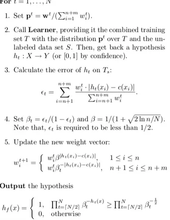
5. Step 5 updates the weights w for the next iteration of the loop. The updating formula is available in the figure. After this step, go back to step 1 for all N iterations.
In order to make predictions, TrAdaBoost has to choose which model, or hypotheses ht, ∀t ∈ [1...N] to use for prediction. The model is selected using the
last formula in Figure 8, which is hard to understand. That formula will be explained later on in this chapter.
Figure 8: Original TrAdaBoost pseudo-code for binary classification
2.4.3 From classification to regression
As we already mentioned, TrAdaBoost was designed for classification. Some points must be changed in order to make it work for regression tasks. These points are:
• In point 4 of Figure 8, εt needs to be 0 < εt < 1. This is a normalization issue
as in classification the |ℎW(')) − X('))| is always between 0 and 1. This does not hold true in regression.
• the Output formula must be adapted to a regression problem.
2.4.4 Normalization
εt needs to be normalized in such a way that it respect the condition 0 < εt < 1.
We report here the error εt formula.
εZ = 1 [ : 4)W|ℎW(G)) − X(G)|) A\] )<A\6 [ = : 4)W A\] )<A\6
wit is the weight assigned at instance i by the tth model; ht(xi) is the output of tth
model over the example xi; c(xi) is the real label of xi. As we mentioned, the
problem of the formula is the part highlighted in red. In binary classification, the absolute error (red part) is by definition between 0 and 1, in regression this does not hold anymore.
Following the suggestion of [47], we modified the above formula. The correction is the next: εZ = 1 [ : 4)W |ℎW(G)) − X(G))| ^ A\] )<A\6 ^ = max| ℎW(G)) − X(G)) |
We take the maximum error (we first calculate the error over all target domain point and then take the maximum absolute value) and normalize all errors using the maximum as the denominator. In such way we ensure all the errors to be between o and 1.
2.4.5 Output function
g = max
W |ℎW(')|
Z is the normalization constant.
The explanation of these formula is rather technical. We leave out the explanation and we point the reader to [48].
2.5 Other data analysis techniques
Data analysis is the process of inspecting, cleaning, transforming and modeling data with the purpose of discovering new information. It encompasses a set of techniques and not all of them must be used in all experiments.
In this section the reader may find different techniques used for data analysis in this thesis.
2.5.1 Data visualization
According to Friedman [49], the “main goal of data visualization is to communicate information clearly and effectively through graphical means”. There is no precise approach or pipeline to follow when it comes to present the data. The most common way is to use plots. Several types of plot exist, some are general purpose, like bar chart, pie chart, some are more specific, like heatmaps. In this thesis we will use the box and whisker plot, which is now presented.
Box plot4, also known as box and whisker diagram, is a standardized way of
displaying the distribution of data based on the five-number summary: minimum, first quartile, median, third quartile, and maximum. In the simplest box plot the central rectangle spans the first quartile to the third quartile (the interquartile range or IQR). A segment inside the rectangle shows the median and "whiskers" above and below the box show the locations of the minimum and maximum.
Figure 9: Box Plots shows the variance of a variable
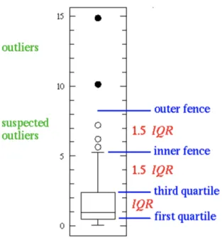
This simplest possible box plot displays the full range of variation (from min to max), the likely range of variation (the IQR), and a typical value (the median). Not uncommonly real datasets will display surprisingly high maximums or surprisingly low minimums called outliers. Two types of outliers are possible:
• Outliers are either 3×IQR or more above the third quartile or 3×IQR or
more below the first quartile.
• Suspected outliers are slightly more central versions of outliers: either
1.5×IQR or more above the third quartile or 1.5×IQR or more below the first quartile.
If either type of outlier is present the whisker on the appropriate side is taken to 1.5×IQR from the quartile (the "inner fence") rather than the max or min, and individual outlying data points are displayed as unfilled circles (for suspected
Figure 10: Box plot showing outliers and suspected outliers
In this thesis we use the box plot to show the distribution of the target collected data (e.g. the gross of movies).
2.5.2 Correlation
Correlation is a statistical measure. Before defining what correlation is, we need to understand what a random variable is. A random variable is a variable which value is the outcome of a random process. It is not possible to know a priori the value of it, we need to observe it. For example, the gross of a movie during his premiere week-end is random variable. We only know the precise value after we have observed it. In this case to observe the value means to sum up all the income of single movie projection. Also, the number of visitors to a Wikipedia page is a random variable.
Suppose now to observe the values of 2 different random variable in pairs. We call the 2 random variables X and Y. X and Y models 2 different random processes, it is not important to know which kind. We observe the pairs (x1, y1),
then (x2, y2), (x3, y3) and so on.
Correlation is a measure of how close 2 random variables are to having a linear relationship. This means that, when correlation is positive, if the values of X increases, the values of Y increases as well. On the other hand, when correlation
is negative, if the values of X decreases, the values of Y decreases. Figure 11 show different examples of correlation, specifically the Pearson Correlation Coefficient.
Figure 11: Plots of a set of data points with shape (x, y). This image is taken from Wikipedia. The value above each plot is the correlation value.
The most used measure of correlation is the Pearson Correlation Coefficient. The Pearson Correlation coefficient r is calculated using the following formula:
q = ∑ (')− 's)(1)− 1s)
A )<6
t∑A)<6(')− 's)7(1)− 1s)7
Where
• xi is the ith observation of variable X
• yi is the ith observation of variable Y
• 's and 1s are the mean of the observations of variables X and Y, respectively. Pearson Correlation Coefficient can range between -1 and 1. Values around 0 means there is no correlation, thus the 2 variables are not linearly correlated. A
the values of the second. Therefore, one variable is almost useless.
On the other hand, a high correlation between and independent variable and the target variable is very helpful as by knowing the values of the independent variable it is possible to predict the value of the target.
2.5.3 Regression metrics
In previous sections we talked about Error, Error metrics and RSS. These metrics are used to evaluate the goodness of the model. In general, error metrics are the way we evaluate how predictions of our model match up against the real values the model is trying to predict.
We already talked about regression and classification. Well, there are other tasks that machine learning is capable, but they are not employed in this thesis. That is to say, for each task, there are also a set of metrics that should be employed in order to assess the goodness of the model. Metrics for classification cannot be used for regression, and vice versa. At the same time, it does not make sense to use metrics for unsupervised learning in a supervised context.
Metrics are also the way to compare different models. The best model is simply the model that performs better. Moreover, not all metrics are created equal: some metrics are more appropriate for some tasks. Models can be compared not only on a single metric, but on a set of them. Different metrics underlines different behaviors of the models.
In this thesis we deal with a regression problem. As such, we now present the most common metrics used in regression. It is important to note that metrics do not care on how the values are calculated. It is not important if the predictions come from a linear regression model or a neural network. A metric only takes as input a set of the values a scores them.
All regression metrics are based on the residual. The residual is the difference between the model’s estimate and the actual value. The residual on the ith
example is
=uvwxyz{ = 1(GK, 3) − ()
Where y(GK, 3) is the model prediction given the features xi and ti is the real
value. Recalling the formula previously presented, the general error is defined as J(3) = :{1(GK, 3) − ()}
D
which happened to be the residual sum. If the residual sum is small it means that, on average, predictions and real values are close and thus the model is good. Conversely, if this residual sum is generally large, it implies that the model is a poor estimator. The reader should note that the previous formula is not actually used as a metric as there are some issues with it.
We are now going to present the metrics that are used in practice.
2.5.3.1 Mean Absolute Error or MAE
MAE is the simplest regression metric possible. Very close the previous formula, MAE is calculated as follows:
|}J = 1
~: |1(GK, 3) − ()|
D
)<5
The residual is calculated over each data point. Then we sum the absolute value of each residual. Absolute value operator is used so that positive and negative residuals do not eliminate between each other. The sum is then divided by the number of examples over which we evaluate the residual. Each residual contributes proportionally to the total amount of error, meaning that larger errors will contribute linearly to the overall error. This means that outliers greatly contribute to the overall error.
2.5.3.2 Mean Squared Error or MSE
MSE is very close to MAE, but instead of using the absolute residual, it squares the residual.