A novel procedure for a typical meteorological year composition with improved resolution adopted in the PV power forecast

(1)

Master of Science – Energy Engineering

A novel procedure for a

Typical Meteorological Year composition with

improved resolution adopted in the PV power

forecast

Supervisor

Prof. Emanuele Giovanni Carlo Ogliari Co-supervisor

Ing. Alfredo Nespoli Prof. Marco Mussetta

Candidate Paolo Sterle – 878579 Academic Year 2018 – 2019

(2)

ii

(3)

Extended Abstract

Acronyms

ANN Artificial Neural Network

E Extraterrestrial Horizontal Irradiance

FS Filkenstein–Schafer statistic

G Global Horizontal Irradiance

MTMY Novel Typical Meteorological Year

PV Photovoltaic

T Air Temperature

TMY Typical Meteorological Year

UR Relative Humidity

V Wind Speed

WO Weighted Occurrences number

WRL Weighted Run Length

WS Weighted Sum of FS statistics

Introduction

Energy sector around the world is undergoing deep transformation, moving from a fossil fuel based industry to a more sustainable approach, founded on renewable energy sources (RES). One of the most diffuse RES is solar energy, which is widely exploited to directly, with Photovoltaic technology (PV), or indirectly, in concentrating solar power systems, generate electricity. Moreover the solar radiation is applied as energy source also in heating systems, hybrid systems, building energy systems and others. However, the incoming power from the sun is not the only factor affecting the performances of such systems, because other meteorological conditions of the environment play similarly a relevant role.

Consequently, in order to characterize a geographical area, it is used the so called Typical Meteorological Year (TMY), a yearly dataset

radiation components and meteorological parameters judged to be typical, on a hourly basis.

The focus of this work is the development of a novel procedure for an improved resolution TMY assembling, which is applied to data collected at the Solar Tech Lab, located in Milano Bovisa.

The dataset generated with the proposed methodology has a wide range of possible applications; here the PV power forecast employing machine learning techniques trained by MTMY is compared to web-available TMY, generated by Photovoltaic Geographical Information Systems (PVGIS). In addition some investigation on the filling technique on a TMY are carried out.

1. Review of procedures for TMY generation

The vast majority of methodologies in literature are based on the idea to select a real sequence of measured data to compose a TMY. This result in a selection of 12 typical months to compose the reference year, as it is done in [1], [2], [3], [4], [5] and others.

The review showed that the most used methodology is the Sandia method, proposed by Hall et al. [1], which make use of the Filkenstein–Schafer (FS) statistical parameter. The procedure is based on an initial dataset composed by 9 daily meteorological variables, for all the available years (15 to 30, depending on the historical measurements). These are reported below:

T max, min, mean

UR max, min, mean

V max, mean

G mean

Table 1: Meteorological variables used inSandia method

(4)

Extended Abstract

iv

According to the description of the method reported by NREL researchers [6], it can be divided into three steps.

STEP 1: For each month of the calendar year, five candidate months are selected having the smallest weighted sum of the FS parameter called WS, evaluated as in eq. 2:

𝐹𝑆#(𝑦, 𝑚) =₊*∑+25*-𝐶𝐷𝐹0(𝑥2) − 𝐶𝐷𝐹4,0(𝑥2)- (1)

𝑊𝑆(𝑦, 𝑚) =₇*∑7#5*𝑊𝐹#∗ 𝐹𝑆#(𝑦, 𝑚) (2)

CDF are the cumulative distribution functions, subscripts y stands for year, m stands for month, x refers to the considered parameter. CDFm is the

long term CDF, evaluated using all the ‘m’ months of the available years. WFx is the weight

factor for parameter x.

STEP 2: The five months are ranked according to the closeness of G and T mean and median of the particular month to the long-term mean and median. The highest relative difference among the four is assigned to the month, as ranking criteria.

STEP 3: The persistence of the mean values of G and T is evaluated, comparing the run (number of occurrences) and the run length (number of consecutive occurrences) above certain threshold limit set on the long-term distribution percentiles. The month with no runs, the month with longest run length and the month with most runs are excluded. The highest month remaining according to ranking at STEP 2 is selected. Many variations have been successively introduced in the original method by researchers. Argiriou et. al. [5] in particular proposed some variations, mainly to account for all the parameters instead of only G and T in STEP 2 and STEP 3. One in particular inspired the procedure proposed in this work, which consider in STEP 2 the weighted sum of relative differences for all the meteorological parameters.

Pissimanis et. al. [4], developed a new approach: its method begins with WS evaluation, as in

STEP 1, then it applies a simpler criteria to rank the selected five months, based on the lowest values of standard deviation s of daily

values of G. 𝜎:= ;∑ (:<=>?) @ + + 25* (3)

In eq. 3 N is the number of days in the considered month and µG the long-term mean.

Lund [2] developed a completely different methodology, based on the assumption that observations of a meteorological parameter are the results of a stochastic process, named Danish method. In addition to the parameters included in Sandia based methods, Danish procedure include also sunshine duration and atmospheric pressure.

Born as a modification of the Danish method, the Festa-Ratto method (Festa and Ratto, [3]) requires a more complex statistical analysis. It is based on the evaluation of standardized residuals X and Z:

𝑋(𝑦, 𝑚, 𝑑) =#(4,0,C)=>D(0,C)

ED(0,C) (4)

X(y,m,d) is the standardized residual of parameter x for the year y, month m, day d, with respect to the long term mean and standard deviation, µx(m,d) and sx(m,d) respectively.

Z is evaluated accordingly to eq. 5 and 6 starting from a first order product between two successive X.

𝑧(𝑦, 𝑚, 𝑑) = 𝑋(𝑦, 𝑚, 𝑑) ∗ 𝑋(𝑦, 𝑚, 𝑑 + 1) (5) 𝑍(𝑦, 𝑚, 𝑑) =J(4,0,C)=>K(0,C)

EK(0,C) (6)

The two exposed parameters are further applied to statistical analysis, and at the end of the process a ‘distance’ is calculated [3], [5], so to consider the typicity of each month. The month with lowest distance is the selected one.

2. PV powerforecast

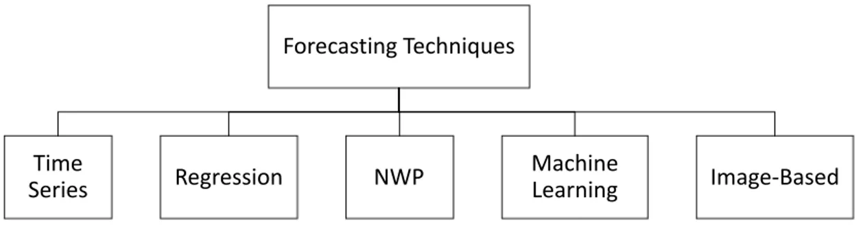
According to Yang et al. [7], the most up to date solar forecasting techniques can be classified in

(5)

five categories: Time series analysis, Regressive analysis, Numerical Weather Prediction (NWP), Image-based forecasting and Machine Learning. In Time series analysis, data are modelled to identify seasonal patterns, trends and relationship with external factors. Times series model are subcategorized; the most used time series method is the Autoregressive Integrated Moving Average (ARIMA) [8].

Regression analysis is a statistical process to estimate functional relationship between dependent and independent variables [9]. Numerical weather prediction (NWP) is a physical model where current observations of weather data, like temperature, relative humidity, irradiance etc. are taken to be used in mathematical model to forecast future data which directly affects solar power generation [10]. NWP is based on empirical relationship between observations and forecasted data. Machine learning is one of the most popular solar forecasting approaches in these days; it guarantees the highest accuracy when applied to PV power forecast [11]. According to Voyant et al. [12], the classification is done on base of supervised learning, unsupervised learning and ensemble learning. Among all these methods, Artificial Neural Network (ANN) is becoming popular by giving better performances compared to other methods.

In hybrid methods, the combination of two or more forecasting techniques is used to improve the accuracy of the forecast.

3. Artificial Neural Network(ANN)

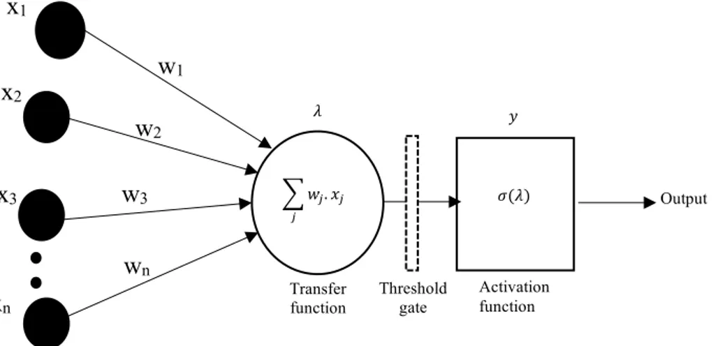
Artificial neural network is a computational tool used for modelling, classification, pattern recognition and multivariate data analysis. Artificial neurons are like biological neurons which are the basic structures of nervous system, containing information and transferring signals from one structure to others.

Basic units of ANN are : Input units, voted to receive data from external source; Output units, which sends data out of neural network; Hidden units, that receives input from previous internal

units, and produce output signals within network [13]. Each unit receives a certain amount of information from the previous layer, and elaborates it through a weighted sum. Weights can be positive (excitation of the neuron) or negative (inhibition of the neuron). The unit output is evaluated by means of the activation function or transfer function, that represent the rate of potential action of the specific unit. Various activation functions can be used, such the sign function, linear or semi-linear function or sigmoid function, reported in Figure 1.

Figure 1: Tan-sigmoid function

Transfer function is activated only if the weighted inputs exceed a certain threshold. The network receives a set of input and a set of expected output, and learns to assign weights and other parameters in order to obtain the expected output as output. Different algorithms can be used to this purpose, the most applied is a back-propagation algorithm [14].

The learning process is divided in training, validation and test. In training the ANN is fed with the training dataset The learning algorithm evaluate the discrepancy between the prediction of the network and the expected output, and moves backward adjusting network parameters in order to decrease the error committed. Validation is employed to give an estimate of model skill while tuning the model’s parameters, consequently the validation error decrease during the learning process. The validation dataset is different from the training one. Test is finally applied, which is simply the final network performance evaluation. In this phase the network receives only the set of inputs, and it reproduce the output. Eventually, the target

(6)

Extended Abstract

vi

output is compared with the output predicted by the ANN, to evaluate the error of the forecast.

4. Case study and experimental equipment

All the data used in the present work were

collected by the instrumentation of the Solar Tech Lab of Politecnico di Milano, whose coordinates are latitude 45.502941°N and longitude 9.156577°E.

The experimental site is equipped with a wheather station, since 2012.

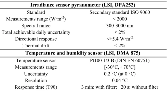
The main characteristics of the sensors are reported in the Table 2 below:

Irradiance sensor pyranometer (LSI, DPA252)

Standard Secondary standard ISO 9060 Measurements range (W·m-2₎ _{< 2000}

Spectral range 300-3000 nm Achievable daily uncertainty < 2%

Directional response <±5.4 W·m-2

Thermal drift < 2%

Temperature and humidity sensor (LSI, DMA 875) Temperature sensor Pt100 1/3 B (DIN EN 60751) Measurements range [-30°C, +70°C] Uncertainty 0.2 °C (at 0 °C) Resolution 0.04 °C

Response time (T90) 3 min: with filter;

20 s: without filter

Table 2: Sensors main characteristics

Among the measured meteorological parameters, only G, T, UR and V were included in the procedure for TMY generation, accordingly to Sandia methodology. Diffuse, beam and global 30° tilted component of solar radiation were also measured, but the lack of some data and the unreliability of others, made the available amount of measures not numerous enough for a TMY generation. As consequence they have been excluded, and filling technique was considered and critically analyzed.

Once recorded in database, the pre-selected variables were assembled on a 10 minutes basis, assigning to the 00:10 (hh:mm) the mean of values between 00:05 and 00:15.

A total of 36 photovoltaic modules of different technologies are installed at solar Tech Lab, with rate power ranging from 75 to 300 W. All modules have are the same Azimuth of the building, which is -6°30’ (assuming 0 as South direction and counting clockwise). The connection to electrical the grid is carried out by micro inverters, one for each module.

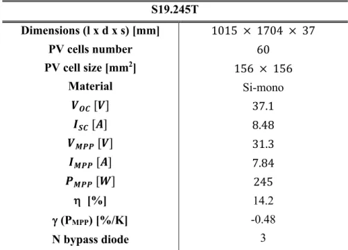
Electric power measures were required in the PV forecast analysis, consequently it was selected a silicon monocrystalline module of 245 W, active since 2013. The technical operating parameters of the module are reported in Table 3

S19.245T Dimensions [mm] PV cells number PV cell size [mm2_] Material 𝑉MN [𝑉] 𝐼SN [𝐴] 𝑉7UU [𝑉] 𝐼7UU [𝐴] 𝑃7UU [𝑊] h [%] g (PMPP) [%/K] N bypass diode 1015 × 1704 × 37 60 156 × 156 Si-mono 37.1 8.48 31.3 7.84 245 14.2 -0.48 3

Table 3 : Technical characteristics of module S19.245T

5. Data Quality Control

A quality control procedure was applied, particularly focused on the solar radiation measurements. The first type of control was a visual inspection, that led to the rejection of data that exhibited evident misleading trend, such as shading errors, and to the adjustment of nocturnal values to null value. Accordingly, one period in particular was entirely removed from the dataset, a sequence of five months in year 2012, referred to as ‘anomaly’.

In the main procedure various tests were implemented, based on the literature. In particular were applied the criteria defined by Journeè and Bertrand [35], since the procedure they proposed was intended to process data with sub-hourly data. G control test investigated

(7)

different aspects: physical limits, of each single ith_{or daily measure, the persistence of daily}

mean µd and standard deviation sd, the rate of

change between two successive measures, Dlimit.

All the threshold limits adopted are reported in Table 4.

In order to take into account the variation of incoming solar radiation during the day, G was divided for the corresponding extraterrestrial horizontal radiation E, which was downloaded from the NREL web-based SOLPOS calculator [54]. Each single G/E value, underwent quality controls, however the values recorded with a solar altitude lower than 2° were not considered.

parameter max min D limit

𝐺 𝐸 1,1 0,03 0,75 𝜇 d𝐺 𝐸eC - 0,05 - 𝜎 d𝐺 𝐸eC 0,35 1 8𝜇 d 𝐺 𝐸eC -

Table 4 : Overview of adopted thresholds for G Regarding T, V, UR, no persistence test was applied; the physical limits that variables had to respect are reported in Table 5, together with maximum allowable rate of change between consecutive measures.

parameter max min D limit

T 40 °C -10 °C 10 °C

UR 100 % 0 % 35 %

V 30 m/s 0 m/s -

Table 5 : Adopted thresholds for T, UR, V

It is worth to be mentioned that also missing measurements have been considered errors, because for the aim of this work it was necessary to know whether a measurement is trustworthy or not, regardless it was missing or wrong. After processing the dataset with quality control methods, results have been analyzed in order to understand the quality of available data.

The data reported to be unreliable, from now on, are referred to as ‘errors’.

The parameter that scored the most number of errors was G, while the most accurate were V and T, as it is reported in Figure 2.

Figure 2: Yearly error percentage of G, T, UR and V

From the errors analysis emerged that three years, 2013, 2017 and 2018, presented a smaller number of error compared with the others. The total error percentage reported in the column on the right in Figure 2, however, is not definitive: the actual rejected amount of data must consider the error overlapping. In fact different tests operated independently one from another on the dataset, therefore different parameters whih referred to the same date and time might had been found to be unreliable by different controls.

Figure 3 : Real percentage of rejected data

Taking into account the overlapping, the actual amount of yearly rejected data is reported in Figure 3, which includes also a long period of anomaly anomaly in 2012. The overall percentage of dataset which did not satisfied the validation criteria is equal to 12,4%, considering the entire seven years period. However the most errors belonged mainly to 2012 and 2016.

(8)

Extended Abstract

viii

6. Proposed procedure

The novel procedure proposed within this thesis, as already introduced, was inspired to a modified version of Sandia method, defined in Argiriou’s work [32]. However, it differs from all classic methodologies because it is aimed to the composition of a TMY with resolution of 10 minutes, and this is reflected by some new passages that were introduced. In order to facilitate the exposition, the TMY generated with the novel procedure is here referred to as Modified Typical Meteorological Year (MTMY).

The first operation was the definition of a strict criteria for error filling: only up to two consecutive errors of G measurements (20 minutes) were filled with linear interpolation. If three or more consecutive values were flagged as unreliable by quality control, no filling was applied, and the data were definitely rejected. In the same way it was done with the other meteorological parameters, but the limit was relaxed to six consecutive measurements (1 hour).

After the filling application, only in 11 months over the available 84 there was a complete absence of errors. However, contrarily to the Sandia methodology, the basic period of time composing the MTMY was chosen to be a five days period of consecutive measurements, instead of one entire month. Such five-days basic unit of MTMY is called here ‘elementary period’, or simply ‘period’. Accordingly, each year was split in 73 periods, only periods entirely composed by reliable data were considered suitable.

Within the proposed procedure, all four the meteorological parameters influence the decisional process that select 73 most typical periods.

The proper procedure is divided in four steps: 1. For each elementary period composing the

calendar year, five candidates are selected having the smallest Weighted Sum (WS) of the

FS statistic of the four meteorological parameters.

In eq. 7 is reported the formulation to calculate FS(y,p,X), of a period p of the year y, for the parameter X

𝐹S(𝑦, p, X) =₊*∑+25*-𝐶𝐷𝐹ij,k(𝑝, i) − 𝐶𝐷Fo(𝑦, 𝑝, i)- (7)

CDFs are the cumulative distribution function, while the subscript LT refer the statistical

distribution to long-term, meaning that it is evaluated considering the period p of all the available years.

𝑊𝑆(𝑦, p) =₇*∑725*𝑊𝐹#∗ 𝐹S(𝑦, p, X) (8)

The formulation of WS, eq. 8, employs a set of weight factors, taken from [33] and here reported in Table 6

X T UR V G

WFx 4/20 4/20 2/20 10/20

Table 6 : Weight factors employed in the procedure 2. The candidate periods are ranked on the base of their closeness of their mean with the long-term mean µLT of the parameters, by means of

the Relative difference Weighted Sums (RWS).

As reported in eq. 9 and 10, µLT is evaluated as

the mean value of N values of µXi(p,Xi), which

is the mean of the ith_{value of the considered}

period over the number of available years n.

𝜇k2(𝑝) =*_p∑p25*𝑋2(𝑝) (9)

𝜇ij(𝑝, 𝑋) =₊*∑+q5*𝜇k2(𝑝, 𝑋2) (10)

RWSs formulation make use of the Relative Difference (RD) between the sample mean and the long-term elementary period sample mean, as in eq. 11 and 12.

RD(y, p, X) = | 𝜇ij(𝑝, 𝑋) − 𝜇(𝑦, 𝑝, 𝑋) | (11)

(9)

3. The persistence of T and G are evaluated by determining the runs (number of occurrence) and run length (number of consecutive occurrences) above and below fixed long-term percentiles, referred to as O and RL. Thresholds for T are the 33rd_{long term}

percentile and 67th_{long-term percentile. G has}

only a lower limit, being the 33rd_long-term

percentile.

In the evaluation of percentiles only values corresponding to daytime measurements have to be considered. This is important since G is always null during night, such behavior would affect the value of the 33rd_{percentile, which}

especially in winter time could tend to zero. Such precaution is applied also to T for coherence of the procedure.

At this point, for each elementary period is calculated the weighted sum of T and G runs and run length beyond the set limits, giving to G a factor 2 in these sums because it has only a lower limit.

In eq. 13 and 14 are reported the formulation of Weighted number of Occurrences (WO) and Weighted Run Length (WRL):

𝑊𝑂(y, p) = 𝑂:(𝑦, 𝑝) ∗ 2 + 𝑂j(𝑦, 𝑝) (13)

𝑊𝑅𝐿(y, p) = RL|(𝑦, 𝑝) ∗ 2 + 𝑅𝐿j(𝑦, 𝑝) (14)

OG and OT stand respectively for stand for

occurrences of G and T outside the limits, while RLG and RLT are the maximum run

length outside the limits in the period p. 4. WO and WRL are used as final exclusion

criteria in the selection process: the two periods with the highest value of these parameters are removed from the ranking at step 2.

Among the remaining periods in the ranking, the one with the lowest RWS is selected to be a part of MTMY.

In the particular case that only two periods are available in the ranking, the selection criteria is based only on the lowest WO.

The process has to be repeated for all the 73 elementary periods.

Once the exposed procedure was applied to the available dataset, the MTMY was assembled. It was composed by periods of all the years. The most represented in the typical composition was 2013, that composed the 24,6% of MTMY.

7. Different ANN training methods and tests

The methodology here applied consisted in evaluating the effectiveness of ANN based by forecast training the network with different TMY datasets, in order to determine which dataset gives the best performances. This pursuit the objective to verify the application of the novel MTMY with 10 minutes resolution generated in the present thesis. Moreover, an investigation on different filling techniques to overcome possible lacking data, which often occur in this kind of problem, was carried out. A generalization of the conclusions of the here presented analysis was obtained by considering also a web available TMY, generated by Photovoltaic Geographical Information Systems (PVGIS).

In order to perform a fair comparison between the methods here analyzed, a strong assumption should be done: performance evaluation was carried out considering the so called “Perfect Weather Forecast” condition, meaning that test dataset was composed by measured values, rather than predicted ones. By choosing this condition, the forecasting errors are deputable to the only methods and not to the weather forecasts inaccuracies.

The description of the applied methodology is divided in three sections.

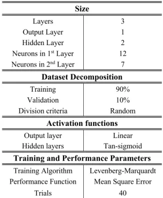
1. Structure of ANN employed

The design of the artificial neural network adopted is very important, because a poor design can lead to misleading results. However in this work ANN are rather considered as on instrument to be used with a pre set optimal

(10)

Extended Abstract

x

design, since many studies were done on the matter [17], [18], [11]. The network architecture and operating parameter employed were taken from [18], and reported in Table 7

Size Layers 3 Output Layer 1 Hidden Layer 2 Neurons in 1st_Layer ₁₂ Neurons in 2nd_Layer ₇ Dataset Decomposition Training 90% Validation 10%

Division criteria Random

Activation functions

Output layer Linear

Hidden layers Tan-sigmoid

Training and Performance Parameters

Training Algorithm Levenberg-Marquardt

Performance Function Mean Square Error

Trials 40

Table 7 : Employed ANN architecture

2. Datasets composition

All the datasets employed in ANN training and test were composed by the same parameters: day of the year, hour, minute, G, T, V and PV power output. The novel MTMY contained also relative humidity values, but in this analysis they were excluded, since UR have a low impact on the PV power output, compared to the others.

In order to create a set of desired output to train the ANN, the power output measurements of the module S19.245T corresponding to each measure composing the MTMY were collected. However, due to technical reasons and accidents in the monitoring activity occurred during the years, only the 33% (120 days) of the measures were collected. As consequence, a filling criteria was implemented. According to Ogliari et. al. [11], machine learning is an effective method to reproduce missing PV power measures having only meteorological variables available. The

ANN based method employed the 33% of reliable data in training and validation, and reproduced the missing 67% electric measures. The PV power values corresponding to the TMY generated by PVGIS, referred to as TMYPVGIS,

were filled with a five parameter physical model, described in [19], which main parameters, experimentally derived from the S19.245 module, are reported in TABLE.

Parameter Symbol Value

Light-generated current IPV [A] 8,659 Current across p-n junction ID [nA] 15,6 Diode ideality factor N [-] 1,208 Module series resistance RS,m [mW] 325 Module shunt resistance RSH,m [W] 1054

Table 8 : Experimental parameters used in physical model [19]

Additionally, a TMYPVGIS reduced version was

assembled in addition, by removing from the dataset the 245 days corresponding to the 67% of missing PV power measures in MTMY. Moreover, to allow coherent comparison with TMYPVGIS, a version of MTMY with hourly

resolution was generated by calculating hourly means of the four meteorological parameters included in the dataset. In Table 9 are reported the main datasets used for training. Subscript ‘H’ stands for hourly resolution, ‘red’ for reduced and ‘fill’ stands for filled dataset.

Name Resolution Days Missing Filling criteria

MTMYH,red 1 hour 120 0% - TMYPVGS,red 1 hour 120 100% Physical _model

MTMYH,fill 1 hour 365 67% ANN TMYPVGIS 1 hour 365 100% Physical _model MTMYfill 10 min 365 67% ANN

Table 9 : Overview of main training datasets characteristics

Test dataset was composed by 92 days of the year 2019, with no missing values of the meteorological parameters and PV power output. Two versions of the test dataset were

(11)

implemented, one with resolution of 10 minutes and one with hourly resolution

3. Results

In order to assess the forecasting methods accuracy, some of the most common error indexes in literature have been considered, including Normalized Mean Absolute Error (NMAE), Enveloped Mean Absolute error (EMAE), normalized Root Mean Squared Error (nRMSE) and Objective Mean Absolute Error (OMAE). The formulations are reported in the following equations: 𝑁𝑀𝐴𝐸 =₊*∑•<‚ƒ-U•,<=U€,< -U_„ ∙ 100 (15) 𝐸𝑀𝐴𝐸 = ∑†‡‚ƒ-U•,<=U€,< -∑†‡‚ƒˆ‰Š (U•,<,U€,<). 100 (16) 𝑛𝑅𝑀𝑆𝐸 =_ˆ‰Š (U* •,<) ;∑†<‚ƒŒU•,<=U€,<•@ + . 100 (17) 𝑂𝑀𝐴𝐸 = ∑†‡‚ƒ_∑Ž-U•,<_|=U€,<-Ž ••‘,< ’“ † ‡‚ƒ . :_“”’ U„ . 100 (18)

In the exposed equations, Pm and Pp are

respectively the measured and the predicted PV power, Pr is the rated power of the module, N is

the number of samples considered in the evaluation and GSTC and GPOACS are the reference

solar irradiance and the clear-sky solar irradiance on the plane of the module.

Performance indexes were evaluated on daily basis, and successively the mean of the 92 days was evaluated.

Firstly, the two reduced version of the hourly datasets, referred to as MTMYH,red and

TMYPVGIS,red, were used for ANN training.

Results showed that the error committed by the ANN forecast was smaller when trained with MTMYH,red rather than with TMYPVGIS,red, which

NMAE value is more than twice higher than NMAE of MTMYH,red, as exposed in Table 10.

Dataset NMAE nRMSE OMAE EMAE

TMYPVGIS,red 2,25 6,73 10,25 14,91 MTMYH,red 0,97 3,49 4,23 8,18

Table 10 : Error indexes of reduced sample dataset The low value of all the error indexes of MTMYH,red based forecast is the prove that the

foreseen PV power output during the test days follows closely the measured power, as reported in Figure 4.

Figure 4 : Forecast and measured PV power comparison

Similar results were obtained training the ANN with MTMYH,fill and TMYPVGIS. In both cases the

NMAE decreased respect to the reduced version of the datasets, as it is noticeable comparing error indexes in Table 11 and Table 10.

Dataset NMAE nRMSE OMAE EMAE

MTMYH,fill 0,88 3,12 3,91 7,29 TMYPVGIS 2,11 6,09 9,72 13,38

Table 11 : Error Indexes comparison

All the different performance indexes confirm the improvement of forecast performances subsequent to an increase in training dataset samples. The reduction of NMAE of MTMY based forecasts due to a 67% reduction in the dataset number of samples, is only of 0,09%. Moreover, this small difference is also an indicator that the filling procedure adopted was effective.

Regarding the performances of network trained with the MTMY with resolution of 10 minutes, it was noted that the NMAE increased to 1,07%, respect to the 0,88% of the MTMYH,fill.

0 5 10 15 20 25 hour 0 100 200 300 400 500 600 GHI [ W/m2 ] MTMY H,red forecast [ W ] measured PV power [ W ] NMAE: 0,516 EMAE: 2,528

(12)

Extended Abstract

xii

Conclusions

The main scope of the present thesis was to propose a novel procedure for TMY assembling, with an improved resolution of data, called MTMY.

MTMY is a yearly dataset, containing four meteorological parameters: air temperature, relative humidity, wind speed and global horizontal irradiance, with resolution of 10 minutes. It can be exploited in many real-time application, especially in the micro-grid optimization process, in the short and very-short term PV power forecast, as well as in pre-sizing phase of all solar energy based systems.

Future works will be aimed to the update of the dataset composition in the next years, including in the initial database the new collected data. As secondary purpose, the assembled MTMY was applied in PV power output forecast, employing a machine learning technique. Forecast performances of MTMY application in ANN training resulted to be mostly accurate, considering different adaptations of the dataset. The best forecast obtained employing a MTMY adaptation reported an NMAE of 0,88%, while the forecast obtained from the classical formulation TMY presented a larger error: NMAE 2,11%.

PV power filling method based on machine learning revealed to be effective.

(13)

Bibliography

[1] IJ. Hall, RR. Prairie, HE. Anderson , EC. Boes. Generation of typical meteorological years for 26 SOLMET stations. Sandia Laboratories Report, SAND 78-1601, Albuquerque, NM, 1978. [2] H. Lund, The design reference year user’s manual. Thermal Insulation Laboratory, Technical University of Denmark, Report 274, 1995.

[3] R. Festa, CF. Ratto. Proposal of a numerical procedure to select reference years. J Solar Energy 1993;50.

[4] D. Pissimanis, G. Karras, V. Notaridou, K. Gavra. The generation of a typical meteorological year for the city of Athens. J Solar Energy 1988; 40.

[5] A. Argiriou, S. Lykoudis. Comparison of methodologies for TMY generation using 20 years data for Athens, Greece. Solar Energy 1999; 1.

[6] W. Marion, K. Urban. User’s Manual for TMY2s Typical Meteorological Years, National Renewable Energy Laboratory, Golden, CO, 1995, USA.

[7] D. Yang, J. Kleissl, C. A. Gueymard, H. T. C. Pedro, and C. F. M. Coimbra, “History and trends in solar irradiance and PV power forecasting: A preliminary assessment and review using text mining,” Sol. Energy, vol. 168, no. November 2017, pp. 60–101, 2018.

hands-on guide. Axelrod Schnall

Publishers, 2018

[9] S. Sobri, S. Koohi-Kamali, and N. A. Rahim, “Solar photovoltaic generation forecasting methods: A review,” Energy Convers. Manag., vol. 156, no. November 2017, pp. 459–497, 2018.

[10] R. Escobar, J. Antonanzas, F. Antonanzas-Torres, R. Urraca, N. Osorio, and F. J. Martinez-de-Pison, “Review of photovoltaic power forecasting,” Sol. Energy, vol. 136, pp. 78–111, 2016. [11] E. Ogliari, A. Dolara, G. Manzolini, S.

Leva. Physical and hybrid methods comparison for the day ahead PV output power forecast. Renewable Energy, Volume 113, December 2017, pp. 11-21. [12] C. Paoli et al., “Machine learning methods

for solar radiation forecasting: A review,” Renew. Energy, vol. 105, pp. 569–582, 2017.

[13] B. Krose and P. Van Der Smagt, “introduction to Neural Networks” J. Biomech., 1996.

[14] B. W. White and F. Rosenblatt, “Principles of Neurodynamics: Perceptrons and the Theory of Brain Mechanisms,” Am. J. Psychol., 2006.

[15] M. Journeè, C. Bertrand. Quality control of solar radiation data within the RMIB solar measurements network. 2010, Solar Energy 85, 72-86.

[16] Solpos web calculator, NREL developer. https://midcdmz.nrel.gov/solpos/solpos.

(14)

Extended Abstract

xiv

[17] A. Dolara, F. Grimaccia, S. Leva, M. Mussetta, and E. Ogliari, “Comparison of Training Approaches for Photovoltaic Forecasts by Means of Machine Learning,” Appl. Sci., vol. 8, no. 2, p. 228, 2018.

[18] A. Nespoli. Development and validation of intra-day photovoltaic power forecast by means of machine learning techniques. Master thesis in Energy Engineering, Politecnico di Milano, 2019.

[19] A. Dolara, S. Leva, G. Manzolini. Comparison of different physical model for PV power output prediction. Solar Energy, Volume 119, pp. 83-99.

(15)

List of Figures

Figure 1. Spatial and temporal resolution of forecasting techniques [2]. ... 4

Figure 2: Classification of forecasting techniques ... 5

Figure 3. Configuration of connection between units ... 13

Figure 4: Types of activation function ... 13

Figure 5. Basic network scheme ... 15

Figure 6. Signal summing in an artificial neuron, the single layer perceptron ... 15

Figure 7. Typical neural network architecture ... 16

Figure 8: Weather station and measurement system at Solar Lab ... 30

Figure 9 : Anomaly in G and D values, data of June 20th_{and June 21}st_{2012 ... 34}

Figure 10: Corrective Factor, taken from LSI technical sheet ... 36

Figure 11: Trend of D and G for 21st, 22nd and 23rd October 2014 ... 37

Figure 12: Shade-band misalignment error for 1st_{and 3}rd_{October 2018 ... 38}

Figure 13: Shading error evidence in June 2012 ... 39

Figure 14: Scatter plot of solar radiation data from Tallahasse, USA, [38] ... 43

Figure 15: Scatter plot of data from Fukuoka, [34] ... 45

Figure 16: Quality envelopes in the Kt-K space, [35] ... 49

Figure 17 : Quality control Algorithm ... Errore. Il segnalibro non è definito. Figure 18: Error percentage of tests including Anomaly ... 57

Figure 19: Yearly error percentage of G, T, UR and V ... 59

Figure 20: Yearly errors overlap ... 60

Figure 21: CDFs of G for 15th period of 2016, from March 12th to 16th ... 69

Figure 22: G period trend comparison for October 25th ... 71

Figure 23: Tan-sigmoid function ... 77

Figure 24: ANN architecture adopted ... 77

Figure 25 : Equivalent circuit representing the five-parameter model ... 82

Figure 26 : NMAE daily error comparison between MTMYH,red and TMYPVGIS,red ... 88

Figure 27 : PV forecast comparison of two consecutive days ... 88

Figure 28 : Best day of TMYPVGIS,red based forecast ... 89

Figure 29 : Best day of MTMYH,red based forecast ... 89

Figure 30 : Worst day of TMYPVGIS,red based forecast ... 90

Figure 31 : Worst day of MTMYH,red based forecast ... 90

(20)

List of Figures

xx

Figure 33 : Example of different meteorological conditions ... 91

Figure 34 : NMAE error comparison between MTMYH,fill and TMYPVGIS ... 94

Figure 35 : PV power forecast comparison of two consecutive days ... 94

Figure 36 : Best day (left) and worst day (right) graphs of TMYPVGIS based forecast ... 95

Figure 37 : Best day (left) and worst day (right) graphs of MTMYH,fill based forecast ... 95

(21)

List of Tables

Table 1: Solar irradiance and sensors characteristics ... 30

Table 2: Technical characteristics of module S19.245T ... 31

Table 3: Meteorological measurements yearly availability ... 33

Table 4: Yearly missing elements ... 34

Table 5: Acronyms [34] ... 46

Table 6: Physical threshold test [35] ... 47

Table 7: Upper and Lower physical limits for T, UR, V ... 53

Table 8: Quality control procedures overview ... 54

Table 9: Number of yearly errors detected ... 58

Table 10: Percentage and number of errors of G, UR, T and V ... 59

Table 11: Number and percentage of errors and rejected data ... 61

Table 12: Rejected data comparison before and after filling procedure ‘O’ original dataset; ‘F’ filled dataset ... 65

Table 13: Frequency and percentage of complete 5-days periods ... 66

Table 14: Weight Factor set, [33] ... 67

Table 15 : Weight factors for MTMY method ... 69

Table 16: MTMY period composition ... 72

Table 17 : Employed ANN architecture ... 79

Table 18 : Parameters used in the physical model [58] ... 83

Table 19 : Overview of main dataset characteristics ... 83

Table 20 : Error comparison ... 87

Table 21 : Performance index comparison between different resolution based MTMY ... 92

Table 22 : Performance index comparison of complete hourly TMYs ... 93

(22)

List of Tables

(23)

Sommario

Negli ultimi decenni il mondo energetico sta affrontando un'intensa transizione della fonte energetica primaria, spostandosi dai combustibili fossili alle fonti energetiche rinnovabili (RES). Uno dei principali settori delle energie rinnovabili è legato all'energia solare: sistemi fotovoltaici (PV), sistemi a concentrazione solare, sistemi energetici degli edifici, sistemi di riscaldamento diretto; sono solo alcune delle applicazioni più diffuse che si basano sulla radiazione solare come fonte energetica primaria.

Al fine di analizzare e prevedere le prestazioni di sistemi basati sull’energia solare nel medio-lungo periodo, data l'imprevedibilità delle condizioni meteorologiche, in molte analisi viene utilizzato un periodo rappresentativo delle condizioni locali, chiamato anno meteorologico tipico (TMY). Si tratta di un insieme di dati aggregato in modo da costituire un anno intero, che include valori di radiazione solare ed altre variabili meteorologiche su base oraria. In questa tesi è presentata una nuova procedura per la generazione di TMY, che modifica la metodologia classica per tenere conto di una elevata risoluzione temporale dei dati. Utilizzando questa metodologia viene quindi assemblato un TMY per la località di Milano Bovisa. Tutti i dati utilizzati sono prima elaborati da un algoritmo di controllo qualità, al fine di includere nell'analisi solo misurazioni di comprovata affidabilità. Tale procedura di controllo è riportata in questo lavoro, cosi come una panoramica delle misurazioni respinte e dei problemi affrontati nel processo di convalida dei dati.

Il TMY generato viene successivamente impiegato per previsioni di potenza di un modulo fotovoltaico (PV) mediante la tecnica dell’apprendimento automatico (Machine Learning). Inoltre, un secondo TMY disponibile online generato secondo la procedura classica da Photovoltaic Geographical Information System (PVGIS), viene utilizzato allo stesso scopo, e l’accuratezza delle rispettive previsioni confrontata. Il metodo adottato per valutare l'efficacia dell’uso di un TMY nella previsione di potenza di un modulo PV è quello di ‘previsione perfetta’. Vengono infine svolte ulteriori indagini sull'influenza di dati misurati e simulati del TMY sulle previsioni.

Parole chiave: Radiazione solare, Controllo qualità dati meteorologici, Metodo di

(24)

(25)

Abstract

In the last decades the energy world has been facing an intense primary energy source transition, from the fossil fuels to the renewable energy sources (RES). Just as the fossil fuel based energy industry relies on reserves, the renewable sector depends upon the assessment of resources. One of the main fields of renewable energy is related to solar energy, which is exploited in different ways, where photovoltaic (PV) systems, concentrating solar power systems, building energy systems, direct heating systems are some of the more assessed application.

In order to evaluate and predict the performance of solar radiation based systems over medium-long time, given the unpredictability of the meteorological conditions, what is considered a typical period is used, known as Typical Meteorological Year (TMY). It is a yearly dataset that includes solar radiation values and meteorological data on hourly basis. In this thesis a novel procedure for TMY generation is presented, which modifies the classical methodology to account for the improved resolution of the dataset. Using this methodology a TMY for the location of Milano Bovisa is assembled. Before the application of the procedure, all meteorological data are processed by a quality control algorithm, in order to include in the analysis only measurements of proven reliability. An overview of rejected measurements and the issues faced in the data validation process are also reported. The TMY generated is later employed in Photovoltaic (PV) power forecast by means of machine learning technique. Also a classical version of TMY, being the web-available generated by Photovoltaic Geographical Information System (PVGIS) is applied to foresee PV power output. Forecast performances are then compared in perfect forecast condition, in order to assess the effectiveness of the TMY employment in PV power prediction. Moreover, further investigations are carried out about the TMY data structure influence over forecast.

Keywords: Solar radiation, Meteorological data quality control, Typical Meteorological

Year (TMY) generation procedure, Photovoltaic power forecast, Artificial Neural Network (ANN)

(26)

(27)

Acronyms

Acronym Description

PV Photovoltaic

RES Renewable Energy Source

TMY Typical Meteorological Year

ANN Artificial Neural Network

MTMY Modified version of typical meteorological year

WMO World Meteorological Organization

NWP Numerical Weather Prediction

TSI Total Sky Imager

ARIMA Auto-Regressive Integrated Moving Average

AI Artificial intelligence

ETS Exponential smoothing

GARCH Generalized Autoregressive Conditional Heteroskedasticity

MLP Multi-Layer Perceptron

LM Levenberg-Marquardt algorithm

UR Relative humidity

T Air temperature

V Wind speed

G Global horizontal radiation

D Diffuse horizontal radiation

B Beam horizontal radiation

B* Estimated beam horizontal radiation

Gt Global 30° tilted radiation

E Extraterrestrial horizontal radiation

(28)

Acronyms xxviii Acronyms Description h Solar altitude K Diffuse ratio Kt Clearness index Kn Beam transmittance FS Filkenstein-Schafer statistic WS Weighted Sum WF Weight Factor

CDF Cumulative Distribution Function

RWS Relative difference Weighted Sum

RD Relative Difference

O Number of Occurrences

WO Weighted Occurrence

WRL Weighted Run Length

e Relative error

MSE Mean Squared Error

NMAE Normalized Mean Absolute Error

WMAE Weighted Mean Absolute Error

nRMSE Normalized Root Mean Squared Error

OMAE Objective Mean Absolute error

(29)

Introduction

A Typical Meteorological Year (TMY) consists of twelve-monthly files of actual hourly meteorological data selected in a particular manner. The months will not, in general, belong to the same year. Instead, each will have been chosen as being a “typical” representative of the month in question and, ideally, the choice for each will have been made from very many years of accumulated data.

The reason for taking actual months of data rather than averaged files is that the former preserve correlations (both known and unknown) that exist among the different measured parameters (e.g. solar radiation and ambient temperature) and also correlations that exist over a period of several days among values of any given parameter. These correlations are often of great importance when one tries to simulate the performance of an energy conversion system that has characteristic timescales of several days (e.g. passive solar buildings, swimming pools, etc.).

The term “typical” is somewhat subjective in that its choice depends, to a large extent, on how the data are to be used. For agricultural purposes it might, for example, be sensible to select typical months on the basis of rainfall and ambient temperature. The present study, however, is part of the meteorological recordings lead in Bovisa Campus since the year 2012, the aims of which are to provide data of relevance to the researchers in the field of solar power stations. Clearly, therefore, the relevant criterion for this purpose is solar energy. There are in fact two solar radiation components that are measured: the global horizontal irradiance (GHI) and the direct beam component, more commonly referred to as the direct normal component (DNI). Since, solar power plants will have to be designed in a manner that will enable them to meet contractual obligations – i.e. to incorporate sufficient backup to overcome such weather fluctuations it is the direct normal component of the solar radiation that is the critical parameter on which the term “typical” must be based.

We expect, therefore, that simulation of a solar power station using one of these TMY files will provide quantitative information about how the system should behave in a typical year. It will not, however, provide any indication as to how the system would behave in an “unusually poor” (from the standpoint of weather) or an “unusually good” year. This information can only come from using data from such years. Again, in an ideal situation where a great many years of data exist, one could construct “unusually poor” and “unusually good” meteorological years in order to meet the needs of such system simulations.

(30)

Introduction

2

Besides, energy sector around the world is under-going deep transformation, moving from a fossil fuel-based industry to a more sustainable approach, founded on renewable energy sources (RES). One of the most diffuse RES is solar energy, which is widely exploited to directly, with Photovoltaic technology (PV), or indirectly, in concentrating solar power systems, generate electricity. Moreover, the solar radiation is applied as energy source also in heating systems, hybrid systems, building energy systems and others. However, the incoming power from the sun is not the only factor affecting the performances of such systems, because other meteorological conditions of the environment play similarly a relevant role.

Consequently, the focus of this work is the development of a novel procedure for an improved resolution TMY assembling, which is applied to real data recorded at the Solar Tech Lab, located in Milano, coupling the weather parameters to the actual power output of a PV module. It should be underlined that the main feature of this work consists on the novel methodology which has been set, in a TMY composition with a larger amount of data, as the weather station provided data which have been averaged every 10 minutes. This modified typical meteorological year composition (MTMY) proposed in this work, is extremely useful in many real-time application, especially in the micro-grid optimization process, in the short and very-short term PV power forecast and all those applications where the hourly discretization is a very long horizon if compared to a minute-scale engineering problem. Hence, the dataset generated with the proposed methodology has a wide range of possible applications.

The current work investigated also the PV power forecast effectiveness on different levels: 1. by employing machine learning techniques applied to the PV output power forecast

exploiting the novel TMY composition.

2. By comparing different filling techniques to overcome possible lacking data which often occur in this kind of problem.

Finally, the conclusions of the here presented analysis have been generalized considering also a web available TMY, generated by Photovoltaic Geographical Information Systems (PVGIS).

(31)

Photovoltaic forecasting review

It is considerably important to predict power generation from Renewable Energy Sources (RES), due to the intrinsic variability of the source. In particular, as regards photovoltaics, rapid fluctuations in power generation affects plant operations in terms of quality and reliability which has direct influence on grid integration and storage balance. The main reasons behind power fluctuations depend on environmental factors, like variation in intensity of solar radiation in case of solar power systems. Such fluctuations can be seen due to many factors including cloud cover or local shadows on PV modules.

In order to face these challenges and gain success, new paradigms have been established with the help of machine learning systems to manage energy consumption and production. Among the first weather forecasting methods, numerical weather prediction (NWP) were adopted in the late 19th_{and early 20}th_{century [1]. The current topic presents the most}

up-to-date state of this dynamic research area, focusing on solar and PV forecasting for medium time horizons.

The basis of modern weather forecasting consists of different sources which are used to evaluate of solar power generation and power forecasting, ranging from measured weather and PV system data to numerical weather prediction models. Depending on forecast horizon, the effectiveness of these resources varies, even though the best approaches used both data and numerical weather prediction model [3].

(32)

Photovoltaic forecasting review

4

Assessment of accurate forecasting depends on numerous factors including local climate, forecast horizon and forecast area.

Figure 1. Spatial and temporal resolution of forecasting techniques [2].

Solar forecasting methodologies are mostly classified into three categories: physical methods, statistical methods and hybrid methods.

In physical methods, physical data are used, such as temperature, pressure, humidity and cloud cover for numerical weather prediction (NWP), also cloud observations by satellite or Total Sky Imager (TSI).

In statistical methods, historical data of solar irradiance are used and categorized into two categories: statistical and learning methods. Seasonality analysis, Box–Jenkins or Auto Regressive Integrated Moving Average (ARIMA), Multiple Regressions and Exponential Smoothing are examples of statistical methods, while AI paradigms include fuzzy inference systems, genetic algorithm, neural networks, machine learning, etc. are examples of learning methods.

In hybrid methods, the combination of two or more forecasting techniques are used to improve the accuracy of the forecast. Therefore, they are also known as combined models. The idea behind the use of hybrid models is to overcome the deficiencies of the individual models making use of their advantages only, merge them together and provide a new hybrid model to reduce forecast errors. For instance, the NWP model can be combined with the ANN by feeding the outputs from the NWP as input to the ANN models. Hybrid models can combine linear models, nonlinear models, or both linear and nonlinear models.

(33)

The classification in this thesis is done based on most up to date forecasting techniques. In order to develop control strategies on PV systems it is important to forecast electricity production accurately, by using forecasting techniques. According to Yang et al. [1], the most up to date solar forecasting techniques can be classified as shown in the figure below.

Figure 2: Classification of forecasting techniques

1.1 Time series analysis

In time series analysis, data are modelled to identify seasonal patterns, trends and relationship with external factors. Nevertheless, in time series forecasting, the information in time series are used to forecast oncoming values, sometimes adding extra information. [4] Time series models are subcategorized in 3 parts, which are:

• exponential smoothing (ETS)

• generalized autoregressive conditional heteroskedasticity (GARCH) • autoregressive integrated moving average (ARIMA)

For statistical forecasting ARIMA and ETS families of models are the most recognizable. On the other hand, the GARCH family of models became popular in econometrics to model financial time series, since the ability of models completes heteroscedasticity corrections [1].

1.1.1

Autoregressive Integrated Moving Average (ARIMA)

ARIMA is the most widely used time series method, primarily used as reference method most of the time because of its broad influence on modern time series analysis and forecasting for both theory and practice [5].

Forecasting Techniques

Time

(34)

6

1.1.2

Exponential Smoothing (ETS)

Exponential smoothing methods originated in 1950s showing a pragmatic approach for forecasting [6]. Exponential smoothing family constitutes various methods, where every single one has characteristic importance to forecast weighted combinations of past observations together with recent observations that are comparatively more weight than previous observations [7].

1.1.3

Generalized Autoregressive Conditional Heteroskedasticity

(GARCH)

A natural autoregressive conditional heteroskedasticity model (ARCH) was introduced by Engle in 1982 with the purpose of observing the change in conditional variance over time as a function of past errors, while leaving constant unconditional variance. However, the need for longer memory and more flexible lag structure led to generalized autoregressive conditional heteroskedasticity (GARCH). GARCH is the extension process of ARCH developed to allow lagged conditional variances in structure [8].

1.2 Regression Analysis

Regression analysis is a statistical process to estimate functional relationship between dependent and independent variables [9]. Regression analysis can be ‘univariate regression’ or ‘multivariate regression’ where the name of regression classification is determined by the number of response parameter involved in. If the only response parameter takes place the regression is called univariate and when more than one response parameter is involved, the regression is called as multivariate.

Simple linear regression and multiple linear regression were widely used and can be very effective for solar power forecasting concerning exogenous variable modelling.

1.3 Numerical Weather Prediction

Numerical weather prediction is a physical model where current observations of weather data, like temperature, relative humidity, irradiance etc. are taken to be used in mathematical model to forecast future data which directly affects solar power generation [10]. It based on empirical relationship between observations and forecasted data.

(35)

Despite the fact that NWP models are popular, because they are open-source and they give high resolution across particular areas, there are many challenges for simulation of solar radiation [1]. These problems can either be caused by underestimate predictions of cloud amount or liquid-water content, or error in clear-sky irradiance [11].

Yang et al. [1] argues that ensemble models, where single model and statistical model are used together, will exploit longer time history.

1.4 Image Based Forecasting

Sky image based solar forecasting is done based on the tracking of the cloud deformation processes, which leads the forecaster to find out the future position and shape of the clouds, giving information about how fast the cloud is approaching to the forecasting area [1], [14]. These forecasting techniques are mostly applied based on satellite imagery or sometimes spatial sky-imagery [1].

1.5 Machine Learning

Machine learning is one of the most popular solar forecasting approaches in these days. The simplest ML algorithm is formed at early 1940s to late 1950s [1]. It was investigated under the computer science and classified as artificial intelligence method. The advantage of this method is that it gives a solution for problems which are impossible to be represented by finding a relation between inputs and outputs [12]. Machine learning models for GHI forecasting may be classified as structural models, time series models and hybrid models [13]. According to Voyant et al. [12], the classification is done on base of supervised learning, unsupervised learning and ensemble learning. Among all these methods, artificial neural network is becoming popular by giving better performances compared to other methods.

Computational Intelligence is largely employed in PV analysis, therefore the most suitable technique to be adopted is selected by investigating most recent developments and researches for solar power systems. Jeong et al. [15] designed and developed prototype models of smart photovoltaic system blind (SPSB) by evaluating PV panel, tracking system and monitoring system analysis.

Hammami et al. [16] conducted thermal analysis to evaluate cell temperature and battery temperature in different environmental conditions, to find out thermal limits in 1D thermal

(36)

8

model using thermal library of Simulink-Matlab, analyzing configuration with or without a set of lithium-iron-phosphate (LiFePO4) flat batteries on the back side of PV module (Battery Energy Storage System BESS). The model validation has been carried out considering the PV module to be at NOCT given by manufacturer, and by specific experimental measurements on the real PV module, including thermographic camera images.

Hong and Yo [17] proposed an enhanced genetic algorithm (GA) to deal with UC and DR, considering uncertain amounts of generated power from renewable sources in the factory power system. The uncertainty of PV power was modeled using stochastic distributions and the problem solved by a two level method: the master level used a novel genetic algorithm, the slave level used the point estimate method, incorporating the internal point algorithm. In order to forecast day ahead power from PV, Grimaccia et al. [18] proposed a general procedure to set up the main characteristics of the network as number of neurons, layout, and number of trials. This was done using a physical hybrid method (PHANN) provided by forecasted meteorological parameters, historical measurements of power production and estimation of clear sky radiation data to perform the day-ahead PV power forecast. The minimum absolute mean error (normalized or weighted) index has been studied to create the most effective configuration for Feed Forward Neural Network (FFNN). The training method is chosen as Levenberg–Marquardt (LM) algorithm, together with slow convergence setting.

Harmony Search (HS) meta-heuristic algorithm was proposed by Guo et al. [19], which includes optimization problem specific to discover optimum tilt and azimuth angle to maximize extraterrestrial radiation on a solar collector in China. The results were compared with a reference group of data obtained by ergodic method conducted in different cities to understand performance of HS. Additionally, particle swarm optimization (PSO) is used to compare the solution quality with the HS algorithm.

Petrone et al. [20] proposed the Genetic Algorithm (GA) to obtain exact solution for SDM parameter identification, requiring only some measured points close to maximum power point (MPP).

Xiong et al. [21] developed symbiotic organisms search algorithm (SOS) to extract parameters from solar cell models. Effectiveness of this model was validated by single diode model, double diode model and PV module model. In addition, to verify the effectiveness of SOS, five state-of-the-art algorithms, including across neighborhood search (ANS), biogeography-based learning particle swarm optimization (BLPSO), competitive swarm optimizer (CSO), chaotic teaching-learning algorithm (CTLA), and levy flight trajectory-based whale optimization algorithm (LWOA), were used for performance comparison.

(37)

Comparison on statistical level is done by the Wilcoxon’s rank sum test at a 0.05 confidence level to identify significant difference between SOS and other compared methods on the same case.

Dolara et el. [22] analyzed the effect of different dynamic and partial shading conditions on PV MPP tracking, which were based on the PSO evolutionary approach MPPT algorithm and compared with classical maximum power point tracking methods, focused to investigate conversion efficiency in conducted scenarios.

Dolara et el. [23] also evaluated different approaches in training data set composition for ANN to be used in physical hybrid method. For ANN, the training algorithm was chosen to be the Levenberg–Marquardt, while the activation function to be the sigmoid, and the number of trials in the ensemble forecast to be 40. Additional performance index (envelope-weighted mean absolute error) is proposed to compare results between different approaches. Mohamed Louzazni et el. [14] performed a comparison among bioinspired algorithms by considering three cases: single diode model, double diode model and photovoltaic module model, to predict solar cell and PV module parameters. The Firefly algorithm was chosen for optimization problem. The results are compared with recent techniques such as the Biogeography-Based Optimization algorithm with Mutation strategies (BBO-M), Levenberg-Marquardt algorithm combined with Simulated Annealing (LMSA), Artificial Bee Swarm Optimization algorithm, Artificial Bee Colony optimization (ABC), hybrid Nelder-Mead and Modified Particle Swarm Optimization (NMMPSO), Repaired Adaptive Differential Evolution (RADE), Chaotic Asexual Reproduction Optimization (CARO) for solar cell single and double diodes; Quasi-Newton (Q-N) method and Self-Organizing Migrating Algorithm (SOMA) for a-Si:H solar cell and the optimal parameters of Photowatt-PWP 201 are compared with the Newton-Raphson Pattern Search(PS), Genetic algorithm(GA) and Simulated Annealing algorithm(SA).

(38)