U
NIVERSITÀ DEGLI
S
TUDI DI
C
ATANIA
D
IPARTIMENTO DIS
CIENZEB
IOLOGICHE,
G
EOLOGICHE EA
MBIENTALIXXIX cycle - Ph.D. in:
Scienze Geologiche, Biologiche e Ambientali
SABRINA GRASSI
Characterization of active tectonic structures of
the Etna volcano, through geophysical surveys,
analysis of site response and deformation.
PH.D.THESIS
Advisor
Prof. S. Imposa
Co-advisor Prof. G. De Guidi
Table of contents
Introduction ... 1
Chapter I ... 6
1.0. Geologic and tectonic framework of Eastern Sicily ... 6
1.1. Foreland domain ... 7
1.2. Mount Etna: volcano-tectonics evolution ... 10
1.2.1. Seismicity of the Etnean area ... 13
1.2.2. Tectonic structures of the Etnean eastern slope ... 16
Chapter II ... 21
2.0. Site response ... 21
2.1. Seismic ambient noise ... 22
2.2. HVSR ... 24
Chapter III ... 28
3.0. Geodetic-topographic monitoring ... 28
3.1. Tacheometry or quick measurement ... 30
3.2. GNSS ... 31
3.2.1. Geodetic datum ... 34
3.2.2. GNNS permanent stations ... 35
Chapter IV ... 38
4.0. Basic SAR principles ... 38
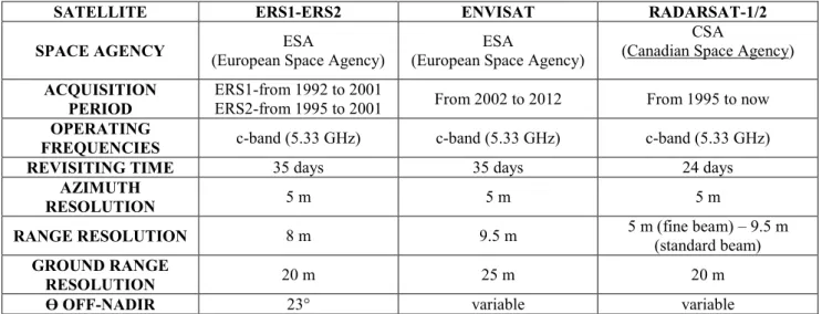
4.1. Satellite systems ... 40
4.2. DInSAR ... 41
Chapter V... 44
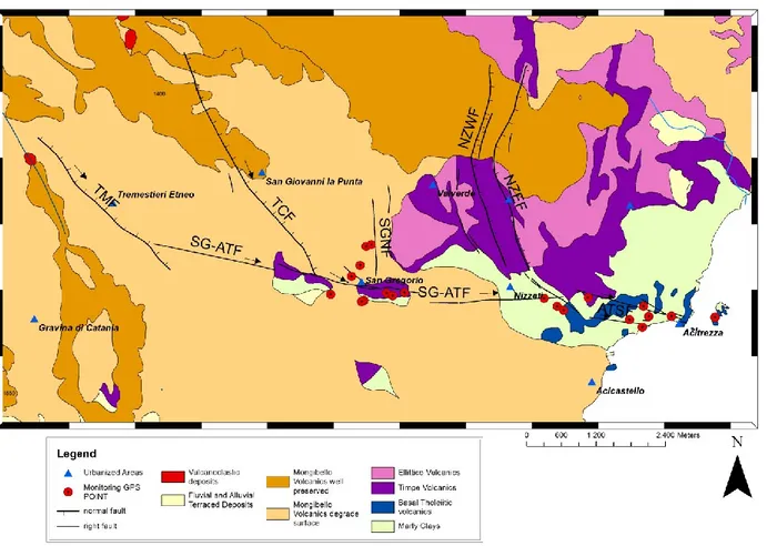
5.0. Tremestieri-Trecastagni-San Gregorio-Acitrezza fault system ... 44
Chapter VI ... 48
6.0. Multidisciplinary surveys in the studied areas... 48
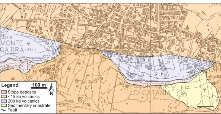
6.1. Surveys in San Gregorio di Catania area ... 48
6.1.1. Structural survey: mapping of the fracture zone ... 49
6.1.2. Geophysical surveys to reconstruct the 3D geological structure of a selected portion of the San Gregorio Fault ... 53
6.1.3. HVSR surveys in San Gregorio area ... 65
6.1.5. Impedance contrast sections ... 78
6.1.6. Topographic and geodetic surveys: monitoring network design ... 84
6.2. Surveys in Tremestieri Etneo area ... 99
6.2.1. HVSR surveys in Tremestieri area ... 101
6.2.2. MASW surveys... 106
6.2.3. Impedance contrast sections ... 108
6.3. Surveys in Aci Castello area ... 113
6.3.1. HVSR surveys in Aci Castello area ... 114
6.3.2. Impedance contrast sections ... 118
6.3.3. Geodetic monitoring of Acitrezza Fault ... 124
Chapter VII ... 129
7.0. Modeling of the slip distribution along the southern boundary of Mt Etna unstable sector: general information to fault geometry construction ... 129
7.1. Construction of the fault system model ... 130
7.2.1. DInSAR data ... 134
7.2.2. DInSAR Kinematic Modeling: slip distribution models ... 138
Discussions and conclusions ... 145
Acknowledgement ... 154
References ... 155
Appendix A. Joint fit MASW-HVSR ... 168
Appendix B. Fit of Vs-depth profiles ... 170
Introduction
1
Introduction
The earthquakes that have affected the Italian territory in the last decade, and the tragic events connected with them, have contributed to stimulate interest in research and development of all those actions that can help to mitigate the seismic risk.
The problems of seismic risk has increased exponentially since the last century, in relation to an increasing of urbanization, which often does not take into account the geological and structural characteristics of the territory. The action planning aimed at the mitigation of seismic risk, which affect a territory, lays its foundations on the studies that allow an improvement of technical-scientific knowledge of the area as well as the assessment of all those parameters which can increase the local seismic hazard.
It is important to study the local and surface geological structures because they determine the site effects, generated by the propagation near the Earth's surface of the seismic waves. It is now widely recognized that local seismic effects can have a significant influence on the extent and distribution of seismic motion and damage during earthquakes.
The local seismic response evaluation is directed to the identification of possible ground motion amplification phenomena that occur when the surface geology is characterized by strong seismic impedance contrasts.
The site effects, are determined primarily by the impedance contrast (defined as the product of the velocity to the density of the medium, in which the wave propagates) that is caused by the seismic wave passage through the rock-soil interface; however, the seismic response varies according to geometrical and mechanical characteristics of the subsoil that are represented by shallow and deep morphological irregularities, vertical and lateral heterogeneity, non-linear and dissipative behavior of ground.
Where are present tectonic structures, it is very important to identify all parameters that contribute to the definition of the seismic response, such as the
Introduction
2
structures geometry, the stratigraphy, the dynamic characteristics of surface soils and the spectral content of a seismic input; these factors contribute to the change in amplitude, duration and frequency content of the ground motion.
The study and monitoring of deformations occurring in seismogenic areas is essential to have a complete picture of the dynamics of these areas. In fact, from the results derived from the study of coseismic or time dependent deformation along shear structures, it is possible to deduce what was the shear event of deformation mechanism and the reaction of the surrounding area, after it occurred.
The studies and the geological and geophysical surveys conducted so far in the Etnean area have highlighted how the subsoil is characterized by considerable lateral-vertical variability of the seismic wave velocity, probably related to the different accumulation geometries of Etnean products; contextually, the different geo-lithological characteristics and the presence of active tectonic structures, strongly influence the local seismic response. Particularly, the Etnean eastern slope is characterized by the presence of numerous active shear structures that present different kinematic characteristics and different modes of strain energy release (coseismic deformation and aseismic creep). These structure can be subdivided into three main fault systems, with different geometry and kinematic (Pernicana Fault System, Timpe Fault System, Tremestieri-Trecastagni-San Gregorio-Acitrezza Faut System), which accommodate the extensional regional dynamic (nearly EW).
I focused the present research on a fault system, considered as "laboratory structure", selected for the different kinematic characteristics and different modes of strain energy release, that characterized the fault segments, identified in Trecastagni-Tremestieri-San Gregorio-Acitrezza Fault System. In the northernmost portion, this system has a kinematic behavior of normal fault and releases energy during coseismic deformation, while in the southernmost portion presents a kinematic behavior of a right-lateral strike-slip fault with releases energy during aseismic creep. Furthermore, this fault system, which can be considered the southern boundary of the sliding of Etnean eastern slope, was less studied than the northern sliding boundary (Pernicana
Introduction
3
Fault system; Alparone et al., 2013; Acocella and Neri, 2005; Siniscalchi et al., 2010, 2012; Bonforte et al., 2007; Currenti et al., 2010; Guglielmino et al., 2011) and very little is known about the depth geometry of its fault segments.
This thesis reports the results of multidisciplinary measurements carried out along the Tremestieri-Trecastagni-San Gregorio-Acitrezza fault system with the aim to provide additional insightful about its geometry and kinematics; also, additional geophysical surveys were performed at various sites of the municipalities most affected by the fault segments in order to obtain information on site response.
The surveys were performed after an analysis of the data relating to surface geology and to morphological, structural, stratigraphic, geophysical and seismological aspects; these detailed surveys have confirmed and highlighted a variety of geological and geomorphological conditions that can determine the occurrence of different stress following the occurrence of an earthquake.
After have performed a detailed structural survey, the project has planned the collection and analysis of many ambient noise acquisitions, and of other geophysical surveys, undertaken within the municipalities affected by the passage of the fault segments, increasing the surveys near the fault. All this in order to reconstruct the resonance frequency distribution and detect the possible presence of areas affected by amplification effects.
Moreover, in some areas, the surface deformation process was characterized through the design, implementation and installation, across the fault segments, of a geodetic monitoring network, in order to obtain information on the fault kinematics and on the local stress field.
The integration of the results obtained from structural, geological and geophysical surveys, with a complete literature review has provided important information on the development in depth of the fault segments; it was thus possible to reconstruct a 3D model of geometry that characterized the southern boundary of Etnean eastern slope sliding.
Introduction
4
Various deformation data such as GPS displacements, InSAR images, level data and measures with extensometers suggest that the slip along the fault system is not uniform, but can be better described by a distribution of dislocation sources along the fault surfaces. In order to model the slip distribution along the fault surfaces, an inverse modeling of DInSAR deformation data was carried out.
This project was aimed to the recognizing site effects, that characterize the studied areas, in order to highlight the seismo-stratigraphic and tectonic behavior of subsoil, as well as to the characterization of the deformation field related to the fault segments, through the implementation of a new geodetic monitoring network (GEO-UNICT geodetic network).
The results allowed to obtain important information on all parameters that can increment the local seismic hazard; all these different but converging approaches, have permitted a complete study of the investigated area. This study providing essential information for a proper land use planning, having as main objective the mitigation of risks that can affect the population.
In addition to the introduction and the conclusions the thesis consists of seven chapters. In the first chapter it is described the geological and tectonic framework of eastern Sicily and the tectonic evolution of the Mount Etna volcano; it is also analyzed the seismicity of the Etnean area, and described the structural framework of the eastern slope of Etna. In the second chapter, the concept of site response is explained and the seismic ambient noise characteristics are discussed; finally it is explained the HVSR (Horizontal to Vertical Spectral Ratio) method and the possibility to obtain information on the seismo-stratigraphic structure of the subsoil.
The third chapter reviews the main geodetic-topographic monitoring techniques, the satellite systems and the geodetic reference systems, as well as the main networks of GNSS permanent stations. In the fourth chapter are explained the basic SAR (Synthetic Aperture Radar ) principles and is briefly examined the space-borne SAR systems evolution; finally it is explained the Differential Synthetic Aperture Radar Interferometry (DInSAR) technique and its importance for the study of the surface
Introduction
5
deformation. The chapter five describes in detail the structural characteristics of the different fault segments belonging to the studied fault system.
In the sixth chapter, for each investigated area are presented the surveys done on the field, the data elaborations and results, both for structural and geophysical surveys and for geodetic monitoring. In the seventh chapter, it is explained how was built the depth geometric model of the fault system and the numerical inversion process used to obtain the modelling of the slip distribution along the fault planes.
1.0. Geologic and tectonic framework of Eastern Sicily Chapter I
6
Chapter I
1.0. Geologic and tectonic framework of Eastern Sicily
The Mount Etna is located in eastern Sicily within the complex geodynamic context of the central Mediterranean area. The resulting tectonic frame is characterized by different structural domains resulting by Neogene-Quaternary convergence of Europe -Africa tectonic plates.
The consequent collision led to the formation of Appennines-Maghrebian orogen. The chain extends roughly in the east-west direction, through the Southern Apennines, the Calabrian Arc, Sicily and North Africa, with south-southeastern vergence (Fig. 1.1).
Fig. 1.1. Geodynamic setting of the central Mediterranean; the arrows show the principal stress direction (red arrows: compressive stress – blue arrows: extensional stress.
1.1. Foreland domain Chapter I
7
The structural setting of Eastern Sicily (Fig. 1.2) is characterized by three different domains: the foreland domain, the orogenic domain and the Tyrrhenian Basin (Fig. 1.3).
Fig. 1.3. Schematic N-S profile (passing through Mount Etna) of the main structural domains of Eastern Sicily ( Lentini et al., 1996, modified).
1.1. Foreland domain
It consists of undeformed portions of the Afro-Adriatic tectonic plates, particularly the Apulian Block and the Pelagian Block are characterized by thickness of about 30 km continental crust. The Apulian Block consists of Meso-Cenozoic carbonate sequences, the Pelagian Block is characterized by slightly thinned crust consisting of Meso-Cenozoic carbonate and volcanic sequences. Between theese blocks is the Ionian Basin, characterized by 11 ÷ 16 km-thick Permo-Triassic oceanic crust, covered by pelagic basin sediments (Finetti, 2005). The foreland domain is represented, in eastern Sicily, from the emerged portion of the Pelagian Block known as Plateau Ibleo; to the east this latter is separated by the Ionian Basin through the Malta Escarpment. It is composed by 300 km-long NNW-SSE oriented normal fault system, extending from Malta up to the southeastern slope of Mount Etna.
Along the foreland northern edge there is the Gela-Catania foredeep, a structural depression formed as a consequence of foreland's margin collapse under the chain. The foredeep is composed by a Neogene-Quaternary sequence of basin deposits that are progressively involved in the orogenic process(Branca et al., 2011).
Fig. 1.2. Main structural domains of Eastern Sicily.
1.1. Foreland domain Chapter I
8
The orogenic domain includes areas characterized by intense deformation, it is divided into three different structural units, the external Thrust System (Carbone and Lentini 1988), the Appenninic-Maghrebian and Kabilo-Calabride Chain, the last two units together make up the allochthonous unit. The deformation process of the external Thust System and the overlap contact of the allochthonous unit, is referred to Upper Miocene-Pleistocene.
The external Thrust System named Sicilian Basal Thrust by Lavecchia et al. (2007) is located along deformed edge of the African-Adriatic plates. It presents a duplex structure involving sequences similar to those of the carbonatic foreland (Lentini et al., 1996; Finetti et al., 1996); its formation, dating Upper Miocene-Pleistocene, is connected to the Tortonian continent-continent collision and to the opening of Tyrrhenian Basin. In this period begins the deformation and the detachment of sedimentary carbonatic coverages of the Pelagian Block margin, earlier inflected under the allochthonous units.
The Apennine-Maghrebide Chain, formed in Sicily the Nebrodi Mountain, and represents the outermost of allochthonous orogenic domains. It is composed of the superposition of sedimentary sequences from the paleogeographic domains originally located between the European and the African Adriatic plates. The Oligo-Miocene orogenic transport was responsible of Chain staking. At the botton of this structural domain, it is possible to observe basinal successions, called Ionidi (Finetti, 2005c), characterized by oceanic crust and ascribable to a branch of the Ionian paleo basin (Finetti et al, 2005a, b; Lentini et al. 2006).
Above the Ionidi Units are present the Panormidi Units composed by Meso-Cenozoic sequences of carbonate platform, characterized by thinned continental crust. Finally, at the sequence roof, represents the Sicilide Units characterised by oceanic crust and consist of Alpino-Tetidee pelagic successions.
The Kabilo-Calabride Chain was originated from the delamination of the European margin, consists of base layers of Proterozoic Paleozoic age, that have superimposed during the Upper Eocene-Lower Oligocene, and by the remains of
1.1. Foreland domain Chapter I
9
sedimentary coverages of Meso-Cenozoic age. The overthrust of this structural domain above the Apennine-Maghrebide Chain coincided with the rotation of the Sardo Corso Block, dating Oligocene-Miocene. In Sicily the Kabilo-Calabride Chain constitutes the frame of Peloritani Mountains.
The orogenic domain overthrusts the Foreland domain areas; its differential feed, gave origin, from Serravallian, on the back of the chain (in inland areas of orogen), to an extensional process, which led to the formation of the Tyrrhenian Basin. The maximum extension has taken place for the basin areas located on the back side of the most advanced orogen portions (Ben Avraham et al., 1990). This differential extension has been accommodated by right lateral strike-slip fault system, arranged en-échelon, oriented NW-SE, then orthogonal to the direction of extension of the chain, known with the name of South Tirrenic System (Finetti and Del Ben, 1986; Finetti et al., 1996). The gradual disappearance of the extension process to the south, along this system, has enabled the advancement of orogenic units of the Calabrian-Peloritan Arc (Lentini et al., 1995) through the Ionian oceanic crust, and the moving back of its slab.
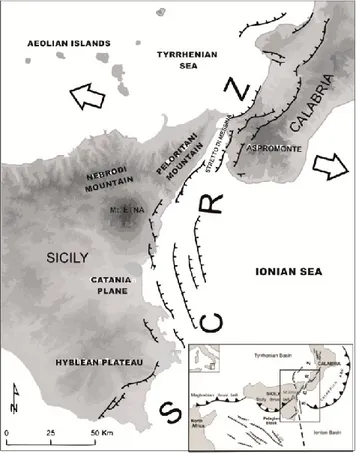
The eastern Sicily is subject to a complex tectonic characterised by the coexistence of two different stress schemes, one compressive NNW-SSE direction, associated to the slow convergence between European plate and African plate, and one extensional stress, that affects the Ionian margin of Sicily and the Calabrian Arc. This extensional zone has about an WNW-ESE orientation (Fig. 1.4) and it is linked
Fig. 1.4. Tectonic Map of eastern Sicily and southern Calabria. The black lines are the main fault segments that make up the Siculo-Calabrian Rift (SCRZ system); the white arrows show the main extension direction of SCRZ system.
1.2. Mount Etna: volcano-tectonics evolution Chapter I
10
to the presence of a fault system known as Siculo-Calabrian Rift Zone (Monaco et al., 1997; Catalano et al., 2008.; De Guidi et al., 2013). This complex system of transtensive faults, characterized by segments of variable length from 10 to 50 km, is long about 370 km; it extends from Calabria's Tyrrhenian coast to reach the Eastern Iblei and the area around the island of Malta (Tortorici et al.; 1995; Monaco and Tortorici, 1995; Monaco et al., 1997; Monaco and Tortorici, 2000). At the Siculo-Calabrian Rift Zone system belong: the fault segments of Maltese Escarpment, the normal faults with right component, localized at the eastern slopes of Etna and the Taormina-Messina fault system.
1.2. Mount Etna: volcano-tectonics evolution
The Etna volcano is located in the convergence area between the European and African plates, along the east coast of Sicily, at the front of the Apennine-Maghrebide Chain and at the footwall of the Malta Escarpment fault system (Monaco et al., 1997), lithospheric discontinuity which, as mentioned earlier, separates the foredeep domain and Hyblean foreland from Ionian domain. With an elevation of about 3330 m and an areal coverage of about 1200 km2, the Mt. Etna is the largest active volcano on the European continent and one of the largest volcanoes in the world. The current Etna structure is the result of a complex interaction between magmatic processes and regional tectonic (Monaco et al., 2010; De Guidi et al., 2012; Azzaro et al., 2013). Another aspect that make complex the structural setting of Etna is related to the variability of the basement on which the Volcano rests; the northern part rests on tectonic units of Apennine-Maghrebide orogen, the southern sector, instead, rests on infra-Pleistocene clay units that fill the Gela-Catania foredeep.
The physical characteristics of Etnean lavas, including thickness and viscosity (Walker, 1967), the chemistry of emission products, initially to tholeitic affinity and subsequently alkaline sodium affinity (Cristofolini and Romano, 1982) and the differentiation trend (Corsaro and Cristofolini, 1996; 1997), set the volcano Etna
1.2. Mount Etna: volcano-tectonics evolution Chapter I
11
within an extensional geodynamic context, that presents WNW-ESE orientation and which is manifested in the Siculo-Calabrian Rift Zone (Tapponnier, 1977; Ellis and King, 1991; Mazzuoli et al., 1995; Monaco and Tortorici, 1995).
The first emission episodes occurred, at the northern edge of the African plate, from the late Miocene (5.3 Ma), they were characterized by extensive lava effusions, with prevailing fissural character, that from the Iblei mounts was subsequently extended to current south-eastern margin of Mount Etna (Branca et al., 2004, 2008, 2011b).
Evidences of the first manifestations of volcanic activity in the Etnean area (pre-Etnean stage: 500-200 ka), are observable at south-eastern margin of the volcano, these are predominantly submarine fissure eruptions, the chemistry of emitted products is transactional tholeiitic (Romano, 1982; Gillot et al., 1994; Monaco et al., 1995).
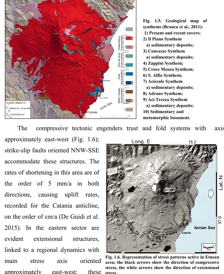
The complex Etnean volcanic succession is characterized by alternating several sequences of lavas and pyroclastic products, originate from numerous eruptive centers that over time have undergone a migration from ESE to WNW (Lo Giudice et al., 1982). The identification within the volcanic succession of strong discontinuities related to the eruptive style change have allowed to distinguish in the evolutionary history of Etna four major phases of activity (Fig. 1.5): Basal Tholeiitic, Timpe, Valle del Bove, Stratovolcano (Branca et al., 2011a, b).
The Mt. Etna presents a complex structure, characterized in the lower part by a shield structure and in the higher-layer by a stratovolcano. To the northwest of the central part of the volcano, the sedimentary basement emerges to 1000 m of altitude s.l.m, consequently, the maximum thickness of the volcanic products in the top portion exceeds 2000 m (Branca and Ferrara, 2013).
The Etnean region is at the center of a complex tectonic system. In the southwestern portion the superficial and profound evidences of a compressive tectonic are visible, with main compressive stress axis oriented approximately
NNW-1.2. Mount Etna: volcano-tectonics evolution Chapter I
12
SSE; this trend appears to be active in the late Quaternary with even current evidence (Monaco et al., 2008; De Guidi et al. 2014, 2015; Ristuccia et al. 2013).
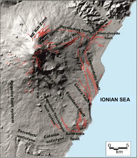
The compressive tectonic engenders trust and fold systems with axis approximately east-west (Fig. 1.6);
strike-slip faults oriented NNW-SSE accommodate these structures. The rates of shortening in this area are of the order of 5 mm/a in both directions, causing uplift rates, recorded for the Catania anticline, on the order of cm/a (De Guidi et al. 2015). In the eastern sector are evident extensional structures, linked to a regional dynamics with main stress axis oriented approximately east-west; these
structures consist mainly of normal faults with horizontal component (right).
Fig. 1.5. Geological map of synthems (Branca et al., 2011): 1) Present and recent covers; 2) Il Piano Synthem
a) sedimentary deposits; 3) Concazze Synthem
a) sedimentary deposits; 4) Zappini Synthem; 5) Croce Menza Synthem; 6) S. Alfio Synthem; 7) Acireale Synthem
a) sedimentary deposits; 8) Adrano Synthem; 9) Aci Trezza Synthem
a) sedimentary deposits; 10) Sedimentary and metamorphic basament.
Fig. 1.6. Representation of stress patterns active in Etnean area; the black arrows show the direction of compressive stress, the white arrows show the direction of extensional stress.
1.2.1. Seismicity of the Etnean area Chapter I
13
1.2.1. Seismicity of the Etnean area
The Etnean area is characterized to an intense seismic activity, connected with the volcano dynamics and the tectonic structures presented therein; also, the Etna region is strongly subject to the effects of the strong tectonic earthquakes at regional character. Among the strongest crustal events, which caused destructive effects in the Etnean area, despite not having hypocenter in this area, there are the earthquakes of 1169 and 1693, with an epicenter in the south-eastern sector of the Hyblean area, and the seismic event occurred in the Straits of Messina in 1908; these events with maximum magnitude of about 7.4, have caused more destructive effects in the eastern side areas (IX-X MCS), and affected less the western and northern areas.
The earthquakes with epicenter in the Etnean area are characterized by a much lower energy content than a regional events, with a magnitude which does not exceed the value 4.9, and hypocentral depths that rarely exceed 10 km, except for the seismic event occurred in 1818, with epicenter in the Aci Sant'Antonio area (CT), of magnitude M = 6.2. This seismic event caused destruction over a wide area of Catania, on the slopes of Etna and in the countries of the Ionian coast, with permanent deformation along some fault zones, liquefaction phenomena, landslides and tsunamis (Boschi e Guidoboni, 2001).
The Etna earthquakes while presenting a energy from low to moderate, because of the extreme shallowness of the source, are capable of causing strong damage to residential areas next to the epicenter; the main effects are recorded in small area (2-5 km long and 1-2 km wide) near the tectonic structure that generated the earthquake (Lo Giudice and Rasà 1992; Gresta et al. 1997; Azzaro, 2004).
A recent scientific paper of De Guidi et al. (2015) highlights a clear deepening trend of hypocenters from shallow depths (0-12 km), in the southern sector of the volcano, to 35 km in NNW sector (Fig. 1.7); this work analyze the seismicity of western and southern sector of the volcano, considering 1900 earthquakes, of magnitude from low to moderate (1.0 ≤ ML≤ 4.8), recorded by the INGV local network between 1999 and 2012.
1.2.1. Seismicity of the Etnean area Chapter I
14 Fig. 1.7. Projection of the hypocentre distribution, relating to the seismic events shown in the lower box on the right (by De Guidi et al. 2015).
The computed focal mechanisms for the main recorded events, in order to characterize the movement type of the seismogenic source and the stress fields actives in the area, has allowed the identification of three areas with different strike-slip regimes.
The deepest zone located to the north of the volcanic edifice is subject to a principal stress σ1 oriented in NNW-SSE direction; the central sector, between 0 and 9 km depth, is characterized by a σ1 oriented E-W; the southern portion, between 10 and 15 km depth, is characterized by a σ1 axis oriented NE-SW (Fig. 1.8).
It is possible be say that, in the west sector of the volcano, at greater depths, the seismicity is strongly influenced by the regional dynamic related to the collision between the African and the European plates, which present the stress axis oriented NW-SE (Cocina et al 1998; Patanè et al. 2003; Scarfì et al., 2013); instead, the seismicity relating to the shallow and middle areas (up to 10-15 km) is affected by local processes, probably related to the volcano dynamics (Latora et al., 1999).
1.2.1. Seismicity of the Etnean area Chapter I
15
Looking at the earthquakes distribution, with a magnitude greater than 3, which occurred from 1990 to 2016 in the Etnean area (Database Isis), it is possible to note that the greatest number of seismic events is localized in the eastern sector of the volcano (Fig. 1.9).
Fig. 1.9. Distribution map of earthquakes with M>3, which occurred from 1999 to 2016 in the Etnean area (Database ISIDe – Italian Seismological Instrumental and Parametric Data-Base). Fig. 1.8. Orientation of stress axes for earthquakes
cluster with hypocentres at different depth (by De Guidi et al., 2015).
1.2.2. Tectonic structures of the Etnean eastern slope Chapter I
16
The seismic events that occur in the eastern portion of the volcano, conversely to those that occur in the west sector, are characterized by hypocenters localized at shallow depths, which in most cases does not exceed 5 km (Gresta et al., 1998); many of the earthquakes that occur in this sector of the volcano can be connected to the activity of surface extensional structures that control the deformation of the Etnean eastern side (Alparone et al., 2013; Azzaro et al., 2013).
The earthquakes of the lower-middle eastern slope of Etna, despite having reduced hypocentral depths, conversely to those that occur in the western portion, are mainly related to regional tectonics, correlated to the extensional regime oriented WNW-ESE to which is subject the east coast of Sicily (Azzaro, 1999; Bousquet and Lanzafame, 2004; Monaco et al., 2005).
The tensile stress to which is subjected this area is differentiated by some authors in regional tensile stress field and local stress field, the latter induced by the gravitational sliding of the slope (Lo Giudice and Rasà, 1992; Walter et al., 2005); in other cases, both regional and local stresses are connected to the opening of the Sicilian-Calabrian Rift (Catalano et al., 2008).
1.2.2. Tectonic structures of the Etnean eastern slope
The eastern side of Etna is characterized by the presence of many fault systems that are the result of iteration between volcanic processes, that take place on a local scale and the complex regional geodynamic pattern, that affect this area with a extensional dynamic oriented ~N100°E (Lo Giudice et al., 1982; Lo Giudice and Rasà, 1986; McGurie and Pullen, 1989).
This domain is confine to north and south by strike-slip shear structures, respectively to north with left movement (the Pernicana system) and to south with right movement, Tremestieri-Trecastagni system (Lo Giudice and Rasà, 1992; Solaro et al., 2010), to west by the North-East Rift (Kieffer, 1975), oriented NE-SW, and by the Southern Rift (Kieffer, 1975), with direction from NS to NNE-SSW (Fig. 1.10).
1.2.2. Tectonic structures of the Etnean eastern slope Chapter I
17
The Pernicana Fault System (Monaco et al., 1997; Azzaro, 1999) extends for approximately 20 km in E-W direction, from Piano Provenzana until the Ionian coast; the fault system shows an extensional character at the surface, while in depth it is characterized by a compressive kinematic due to the overlap of the Apennines on the Hyblean block. To confirm the hypothesis of a compressive regime, under this structure, there is an outcrop of the Quaternary marine deposits at higher altitudes above 700 m, which cannot be justified by the kinematics of the coastal fault systems that lower to east towards the Ionian basin. In the eastern portion this system is characterized by structures with en-échelon trending and development about parallel to each other and with ESE direction, that arriving near the coast. The structure known as Fiumefreddo Fault belongs to this fault system, it extends about in E-W direction and has a left-lateral strike-slip movement (Azzaro et al., 1998a; Tibaldi and Groppelli, 2002). The seismic sequence that preceded the early stages of the eruptive
IONIAN SEA
1.2.2. Tectonic structures of the Etnean eastern slope Chapter I
18
activity generated along the northeastern rift, in October 2002, can be related mainly to the activation of the Pernicana Fault, in its westernmost segment, and it is precisely in this area that the most energetic events (M = 4.2) have been located. The fault throws observed in that occasion were of the order of 20-25 cm for vertical ones and 10-15 cm for horizontal ones. The eastern sector of the fault system is well identifiable due to fracturing phenomena of road surface, walls and various artifacts, affected by phenomena of aseismic creep with left-lateral transtensional movement of the order of 2 cm/a (Rasà et al., 1996; Groppelli and Tibaldi, 1999; Azzaro et al., 2001).
The Rift System of the southern slope, ends along a cutting area with right-lateral movement, known as Trecastagni-Tremestieri System, which consists of a series of segments arranged en-échelon, with NW-SE direction (Monaco et al., 1997). The Trecastagni and Tremestieri structures are two normal faults with right-lateral component, characterized by evident morphological escarpments sometimes obscured by the presence of slag cones and recent lava flows. In the Trecastagni Fault have been observed coseismic displacements of the fault scarp both during the seismic sequence of September 1980, both in consequence of the earthquake of 11/21/1988.
As a consequence of this seismic events it was possible to observe subsidence of the soil, cracks along the SP 8/III walls and on buildings (Azzaro, 1999). By some SAR interferometry studies made by Froger between 1996 and 1998, were estimated displacements to year of about 4-6 mm, but with the eruption crisis of the 2001-2003, as observed for the Pernicana Fault System, has been registred a growth of fracturing on manufactured and an increase of the annual movements that have become from millimetric to centimetric.
The south-central area of the lower east side of Etna is characterized by the presence of a major fault system that extends for about 30 km, known as Timpe system. This system consists of normal faults, with right lateral component, oriented NNW-SSE/ NW-SE, which dip to the east; these structures create steep morphological jumps with vertical throws that in some cases exceed the hundred
1.2.2. Tectonic structures of the Etnean eastern slope Chapter I
19
meters. A number of major segments belong to the Timpe system (Fiandaca, Acireale, Santa Tecla, Moscarello and San Leonardello), some of these have been responsible for well-known destructive earthquakes that occurred in the area: S. Tecla-Linera Fault for the earthquake of 1914, Moscarello Fault for the seismic events of 1865 and 1911, Macchia Fault for the earthquake of 1989, Fleri Fault for the seismic event that occurred in 1984 and Santa Venerina Fault for the earthquake of 2002.
From a morphostructural point of view this system is composed of juxtaposed primary structures from synthetic and antithetic faults that, in some cases, form “graben” structures, as in the case of the San Leonardello Fault.
The northernmost area of the lower east side of Etna is characterized by the presence of a further fault system oriented NNE-SSW, connected with the Timpe system, known as Piedimonte system; it consists of some normal faults, which dip towards east. Three are the main segments that belong to this system: Piedimonte Fault, Calatabiano Faults and Ripe della Naca Fault. The first two structures, oriented respectively, WSW-ENE and NE-SW, are interpreted as regional tectonic lineaments (Finetti et al., 2005; Lentini et al., 2006). The Ripe della Naca Fault is composed by a pair of escarpments, with height between 80 and 120 m (Azzaro et al., 2013), oriented WSW-ENE. The Ripe della Naca and Piedimonte structures are buried by Holocenic lava flows and interrupted by the Pernicana Fault (Azzaro et al., 2012).
Structural analyses of different fault segments on the eastern Sicily and geodetic measurements allowed to determinate the mean direction of extension (~N115°E) and an opening velocity of 3.6 ÷ 0.6 mm/a (Monaco et al., 1997; Monaco and Tortorici, 2000; D’Agostino and Selvaggi, 2004; Catalano et al., 2008).
In the Etnean eastern slope single fault segments and volcano-related processes make more complex the overall tectonic setting (Catalano et al., 2004; Catalano and De Guidi 2003; De Guidi et al., 2014; Scudero et al., 2015). An uplift rate of 2.5–3.0 mm/a has been estimated for the last 6–7 ka along the eastern coastal slope of Etna (Branca et al., 2014). The general process of uplifting is only locally interrupted by
1.2.2. Tectonic structures of the Etnean eastern slope Chapter I
20
subsidence related to flank sliding of the volcanic edifice, measured at manmade structures, and by up rise acceleration along the hinge of an active anticline and at the footwall of an active fault (Branca et al., 2014). GPS and PSInSAR data show a more marked subsidence, (Bonforte and Puglisi 2006; Bonforte et al., 2011).
Many authors have interpreted the Etnean tectonic structures as the boundaries of some independent blocks moving consequently to the gravitational spreading of the eastern flank of the volcano (Borgia et al., 1992; Rasà et al., 1996; Rust and Neri, 1996; Froger et al., 2001; Tibaldi and Groppelli, 2002; Neri et al., 2007; Palano et al., 2008; Palano 2016).
Other authors indicate different causative factors (regional stress, gravity forces and dike-induce drifting, or a combination of these) to explain the slow sliding of eastern and south-eastern flanks (Bonforte et al., 2013). Branca et al. (2014), highlight that the sliding-related subsidence clearly involving the northern eastern sector of Etna has only recently affected the southeaster sector of the slope, where it failed to counteract the effects of the volcano-tectonic uplifting. The time–space boundaries of the lateral sliding, which is probably much younger and shallower than is generally stated and differentially involves distinct blocks, remains to be constrained more accurately.
2.0. Site response Chapter II
21
Chapter II
2.0. Site response
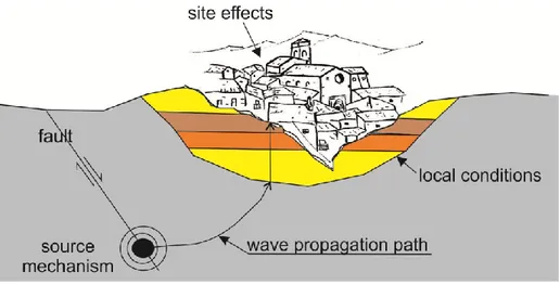
The mechanical and physical properties of subsoil as well as their stratigraphic and morphologic features influence the seismic ground motion recorded at the free surface. The seismic shaking U(t) can be considered the results of the superposition of three different factors: the source mechanism S(t), the seismic wave propagation from the bedrock to the site A(t) and the site effects G(t).
U(t)= S(t)*A(t)*G(t)
The first two factors define the kind of seismic input whereas the third represents all modifications that can occur as a consequence of the interaction between seismic waves and local features of the site.
Fig. 2.1 . Factors which determine the seismic motion at the site.
It is well known that the seismic waves undergo a first change of spectral composition during the source-bedrock path (attenuation function), and a second, when they cross the layers between the bedrock and the free surface; the latter is known as “local seismic response”.
The site effects are determined primarily by the impedance contrast (Z), defined by the equation:
2.1. Seismic ambient noise Chapter II
22
were V is the seismic wave velocity and ρ is the density of the medium in which the wave propagates; it is a parameter closely related to the amplification of seismic vibrations that is caused by the passage of seismic wave through the interface between rocks with different physical and mechanical characteristics. The seismic response varies according to geometrical and mechanical characteristics of the ground: superficial and deep morphological irregularities; vertical, horizontal and lateral heterogeneities; non-linear and dissipative behavior of the soil.
The local conditions, such as the different mechanical properties of the subsoil linked with the presence of discontinuities, fractures or heterogeneities, as well as the geometry of shallow layers and the surface topography affect the propagation of seismic waves causing several physical phenomena as diffraction, multiple reflections, resonance etc. This phenomena can cause local seismic amplification effects, linked to changes of seismic motion and its frequency content.
The local seismic response determines the different damage distribution in various areas affected by the same seismic event.
The site seismic response can be evaluated by experimental method using the records of seismic signals generated by ambient seismic noise.
2.1. Seismic ambient noise
The seismic ambient vibrations are constantly present on Earth’s surface; they are characterized by seismic waves of low energy and amplitudes of the order of 10-4 - 10-2 mm (Okada, 2003).
The seismic noise is originated by a series of different sources, often not related and continuous, distributed spatially. For these reasons the noise is compared to a stationary stochastic process, which is devoid of a well-defined phase spectrum (Bormann and Wielandt, 2002).
The seismic ambient noise sources can be natural or anthropogenic, this subdivision is carried out as a function of their frequency.
2.1. Seismic ambient noise Chapter II
23
Natural sources essentially act at low frequencies (<1 Hz) and anthropogenic ones at high frequencies (>1 Hz). The vibrations with low frequencies (<1 Hz) are called microseisms, while those at high frequencies (>1 Hz) are known as microtremors.
The microtremor sources are largely due to cultural activities such as industrial, agricultural, and traffic noise. They energize the soil mainly with surface waves, which lessen within a few kilometers, both on the surface and at depth (McNamara and Buland, 2004).
Signals below 0.3 Hz are primarily caused by oceanic waves, winds and other meteorological sources (Bonnefoy-Claudet et al., 2006a). The interaction between marine wave and coasts induce the propagation of elastic waves within the continental crusts.
Ambient noise has a temporal variability (Okada, 2003) linked to the different types of sources generating it; at frequencies below 1 Hz, it is linked to the succession of meteorological phenomena, while at higher frequencies ambient noise is frequently affected by anthropic activity. The amplitude of the noise does not particularly vary in a few hours, but seems variable for samplings made on different days (Okada, 2003)
Seismic ambient noise can be considered the result of the interaction of several unrelated seismic sources (Lachet and Bard, 1994; Tokimatsu, 1997; SESAME, 2003). Many authors assume that ambient noise consists mainly of seismic surface waves (Ohmachi and Umezono, 1998; Chouet et al., 1998; Yamamoto, 2000; Arai and Tokimatsu, 1998, 2000; Cornou, 2002; SESAME, 2003) and that the proportion between the wave types depends on the site conditions and the impedance contrast (Bonnefoy-Claudet et al., 2008).
Ambient noise has, in recent years, become widely used for site amplification studies.
The vertical seismic component is conditioned by the Rayleigh waves, while the horizontal components are influenced simultaneously by Rayleigh and Love waves
2.2. HVSR Chapter II
24
(Aki and Richards, 2002; Lay and Wallace, 1995). The H/V ratio can therefore be considered indicative of Rayleigh waves ellipticity (Bonnefoy-Claudet et al., 2006a, b), and the ellipticity curve shows a peak corresponding to the site fundamental frequency (Lachet and Bard, 1994; Kudo, 1995; Bard, 1998).
The presence of Love waves does not alter this interpretation, since the Airy phase that occurs at a similar frequency to the fundamental frequency, acting on the horizontal components, strengthens the peak (Arai and Tokimatsu, 2000). The propagation of Love waves in the environmental seismic noise controls the HVSR amplitude (Bonnefoy-Claudet et al., 2008).
2.2. HVSR
The “passive seismic single-station” method provides information on the local seismic response and it is based on the acquisition of environmental seismic noise.
The main advantage of this methodology is related to its non-invasiveness and quick execution, since it does not require any artificial energization.
The analysis of the record of seismic noise can be carried out by several methods; among these, the technique known as H/V Spectral Ratio is the most used. This technique allows identifying the frequency at which ground motion is amplified due to resonance effects, related to the presence of tectonic and stratigraphic discontinuities as well as the topography (Dal Moro, 2012), by calculating the spectral ratio between the average of the horizontal components on the vertical component of the ground motion.
The HVSR technique, applied for the first time by Nogoshi and Igarashi (1970), was analyzed and made widespread by Nakamura (1989). The frequency of the maximum H/V amplitude corresponds to the fundamental SH resonance frequency of the site. Indeed, the peaks occurring in the H/V spectra indicate the resonance frequencies proper of the site, while their amplitude gives information about the minimum expected seismic amplification at the site in case of earthquake.
2.2. HVSR Chapter II
25
It is known that stratigraphy, topography (surface and buried morphology) and geotechnical characteristics (static and dynamic properties of the subsoil) of a site, may play an important role on the site effects linked to earthquakes, by locally attenuating or amplifying the expected ground motion at the surface compared to the reference bedrock (Albarello and Castellaro, 2011).
The HVSR peak is linked to an impedance contrast in the subsoil with varying amplitude depending on the degree of this contrast. Although the relationship between the two variables is nonlinear, the higher the values of the impedance contrast between different rock types, or between portions of the same lithotype with different mechanical characteristics, the greater the amplitude of the spectral peak. Many authors (Yamanaka et al., 1994; Duval et al., 1995; Goula et al., 1998; Bodin and Horton, 1999; Zhao et al., 2000; Giampiccolo et al., 2001; Panou et al., 2005; Pappalardo et al., 2016) have shown how the HVSR technique is well suited to identifying the impedance contrasts created at the transition between rock types with different physical–mechanical characteristics.
The records of ambient noise, through the H/V spectral ratio technique, can supply information on the mechanical behaviour of buried structures under seismic stress. This technique can be considered an important tool for a preliminary characterization of the local seismic response, since it allows highlighting the main seismic refractors (Spizzichino et al., 2013).
Each peak in the H/V graph corresponds to a possible reflector (seismo-stratigraphic level) that presents an impedance contrast compared to the neighbour levels. Since the impedance contrast may be related to stratigraphic variations (Amorosi et al., 2008), and the stratigraphy of a rock sequence may consist of alternation between intact and fractured layers (Gross, 1995), the H/V single-station technique could provide information also about changes in the degree of fracturing of the rock sequence. In this case, the impedance contrast occurs between layers with different geomechanical properties (Pappalardo et al., 2016).
2.2. HVSR Chapter II
26
In a simple two-layer system of soft sediment, with a shear-wave velocity Vs and a thickness H, covering a hardrock basement, the equation (1) links the resonance frequency “f” to the thickness “H” of the resonating layer, depending on the shear waves velocity:
f = n Vs/4 H (1)
where n (= 1, 3, 5...) indicates the order of the mode of vibration (fundamental, first superior, etc.), Vs and H represent the shear waves velocity and the thickness of the resonating layer respectively.
Equation 1 allows understanding how the H/V technique can also provide information on stratigraphic features. Starting from a noise measurement providing f, once known the Vs of the coverage, the depth of the main seismic reflectors or vice versa can be estimated.
In recent years, this method has been widely used to obtain information on the subsoil stratigraphy (Field and Jacob, 1993; Lachet and Bard, 1994; Lermo and Chavez-Garcia, 1993; Bard, 1998; Ibs-von Seht and Wohlenberg, 1999; Delgado et al., 2000; Parolai et al., 2002; Imposa et al., 2013, 2016a,b; Pappalardo et al., 2016; Tarabusi and Caputo, 2016).
It is reasonable to consider that the waves velocity within the investigated medium increases with depth due to a greater consistency of the material, associated with increasing load. This relationship can be expressed by the following function (Ibs-von Seht and Wohlenberg, 1999):
(2) where:
Vs(z)= shear wave velocity V0= shallow shear wave velocity
z= depth
2.2. HVSR Chapter II
27
Knowing the velocity change with depth, determined experimentally, it is possible to obtain the parameters V0 and α for which there is the minimum error
between the experimental Vs - depth profile and curve fitting these data. Substituting these two parameters in the formula of Ibs-von Seht and Wohlenberg (1999), it is possible to convert the frequency values in depth values:
(3)
This process enables reconstructing the impedance contrast sections that show the distribution of the amplitude values of the H/V spectral ratio in the subsoil.
In order to detect the presence of directional effects on HVSR peaks, the spectral ratio must be calculated along various directions (Albarello, 2005), turning the NS and EW components of the motion with azimuthal intervals of 10°, proceeding from 0° (north) to 180° (south).
3.0. Geodetic-topographic monitoring Chapter III
28
Chapter III
3.0. Geodetic-topographic monitoring
In a geodetic monitoring network, the area or object under investigation is usually represented by points which are permanently monumented or marked. All these points are observed from two to
several times in different time epochs. A geodetic network can be a terrestrial network, a Global Positioning Satellite (GPS) network or a combination of these network types.
In topographic monitoring the changes are measured and analyzed over time, in terms of direction, distance and
difference in height, among points, identified as targets.
The measure of direction is defined by three different angles: direction angle, azimuth angle and zenith angle. The direction angle is the angle between reference direction and the measured direction. Considering a Cartesian coordinate system, where the coordinates of two points A and B are known (Fig. 3.1), we define "angle of the direction of B with respect to A (θAB) or (AB)", the angle made
by the clockwise rotation of an axis parallel to the Y axis, passing through the reference A, to overlap the direction AB.
θ
BA is the reciprocal of θAB.Fig. 3.1. Direction angle
3.0. Geodetic-topographic monitoring Chapter III
29
Considering three points A, B, C (Fig. 3.2a) the azimuth angle is the dihedral angle formed by the plane containing the verticals passing through A and B with the plane containing the verticals passing through A and C.
The zenith angle φAB is the angle between the direction of the vertical passing
through νA and the considered direction ZAB (Fig. 3.2b).
The angle unit is the "radiant" [rad], defined as "the angle subtended by an arc equal in length to the radius"; it follows that the angle αr is expressed in radians as αr
= l / R, where l is equal to the length of the arc subtended and R is equal to radius circumference. In the centesimal system the unit is the "centesimal degree" [gon], defined as 1 gon = π / 200 rad. In the sexagesimal system the angle unit is the "degree sexagesimal" [°], defined as 1° = π / 180 rad.
Defining the position of a discrete series of points, with high accuracy, is the basis of a good topographic monitoring, because all the measures will be related to the position of those reference points. This points are called vertices (benchmarks); they allow to properly insert the land survey in a defined reference system (local or national).
The main network represents the structure within which are located other subnets that allow a detailed topographic survey; this network defines the local reference system to which the other subnets are linked. The main network is determined with redundant measurements, for allowing statistically strong controls. The coordinates of its points are identified as reference (are considered fixed), because the main network is considered as infinitely precise.
Secondary networks and those of detail can also be calculated and compensated independently, in their own system of reference, and later incorporated into the general system of local survey with appropriate transformations.
The construction of the main reference network is carried out through the triangulation method; to determine the coordinates of an inaccessible point, the network of known points, through the basic triangulation, can be thickened with the operations of forward intersection and reverse intersection.
3.1. Tacheometry or quick measurement Chapter III
30
In the topographic survey called simple polygonal, the coordinates of the intermediate vertices of a broken line, formed by "n" segments, are determined starting from two known endpoints (belonging to the main monitoring network or derived from that network through forward intersection or reverse intersection).
The coordinates of the intermediate vertices are determined by measuring their mutual distances and angles formed by the segments that join them. In order to perform a polygonal, between two points on the reference network, it is necessary to choose and materialize on the ground the points “P” which represent the vertices.
The scheme of the open traverse bound to extremes (Fig. 3.3) shows two extreme vertices (A-B) with known position (for example, determined by GPS measurement), the position of intermediate vertices is determined measuring all sides and all angles, in every point of the polygonal it is measured the previous point and the next point.
The scheme of the closed traverse (Fig. 3.4 ) shows that in this case the last side is coincident with the first.
3.1. Tacheometry or quick measurement
Tacheometry is a method of measuring both horizontal distance and vertical elevation of a point in the distance; it represents the last phase of the topographic survey because it allows to identify the detail points. In order to carry out the survey
Fig. 3.3. Open traverse
3.2. GNSS Chapter III
31
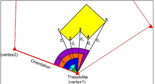
with this method are necessary a theodolite and a diastimeter. The methods discussed above are used to determine the vertices of a monitoring network; in the tacheometric survey the points to be detected may correspond to architectural elements, such as edges or manmade details.
The survey is made in a reference system bound to the coordinates of two vertices used, one for positioning the theodolite (station point) and the other as orientation (Fig. 3.5). By collimating the sequence of vertices to be determined it is possible to define the coordinates of these vertices by measuring azimuth, zenith and distance.
Fig. 3.5. Scheme of tacheometry surveying
3.2. GNSS
GNSS (Global Navigation Satellite System) (Fig. 3.6) is a satellite system that is used to pinpoint the geographic location of a user's receiver anywhere in the world. It is based on the emission of electromagnetic signals which allow to obtain information related to time and distances between satellites and a receiving station. Through the reception and interpretation of such signals by small electronic receivers, located on the earth's surface or in the atmosphere, it is possible to determine the position in a
3.2. GNSS Chapter III
32
predetermined reference system (longitude, latitude and altitude). Two GNSS systems are currently fully in operation.
NAVSTAR GPS (Navigation Satellite Timing And Ranging Global Positioning System) is a spatial navigation system developed by the United States Department of Defense, capable of accurately estimating the position, velocity and time in a common reference system. The constellation is formed by 24 satellites, located on 6 orbits, tilted 55° to the equator and designed to allow the visibility of up to 12 satellites at the same time, from any location on Earth, at any time of day or night.
GLONASS (Global Navigation Satellite System) is a spatial navigation system of the Russian Federation. It is composed by 14 satellites simultaneously visible on the horizon.
A third, the European Galileo, is slated to reach full operational capacity in 2020; as of May 2016 the system has 14 satellites in orbit. When Galileo will be fully operational, there will be 30 satellites in Medium Earth Orbit (MEO). Ten satellites will occupy each of three orbital planes inclined at an angle of 56° to the equator.
The positioning can be performed using two different techniques: the "Point Positioning", which consists in the absolute positioning of a single point in the assigned reference system, this method determine the position with an uncertainty of the order of tens of meters; the “Differential Positioning” or “Relative Positioning” method determines the position of a point with respect to another, considered as known, with a precision of the order of a few millionths of the distance. In particular, the vector relative position of the "baseline" between the two points is determined in
Fig. 3.6. Orbital information about GNSS and other systems
3.2. GNSS Chapter III
33
its three components with respect to an assigned Cartesian tern. In order to utilize this second technique two receivers (base + rover) located on two different points and operating simultaneously for the entire duration of the measurement session are necessary. The time of the measurement session is variable depending on the distance between the two receivers and the accuracy required.
The positioning is carried out through distance measures between the satellites, with known position, and the monitoring points on the earth's surface; the measurement accuracy depends on various factors, such as the number and geometry of satellites tracked, observation time, ephemeris, ionospheric and tropospheric conditions, multipath etc…
The main acquisition methods utilized for geodetic-topographic monitoring with GNSS systems are: static, kinematic and real time kinematic (RTK).
In the static method the measures have a variable time from 30 minutes to several hours, in this case the receivers are kept fixed on the ends of the baseline to be determined; this method provides high accuracy data (3 mm in the horizontal component, 5 mm in the vertical component).
In the kinematic method one of the two receivers (base) is maintained on a fixed position and the second (rover) is moved over the points that must be measured, following a path with continuity, the determination of position is performed at regular time intervals.
These two methods require a post-processing phaseof the measures.
In the RTK method, similar to the operating mode of the kinematic method, the determination of the points position is performed in real time, at the moment when the point is occupied by the mobile receiver. The fixed receiver (normally placed on a known position) communicates its position and the satellite data to the mobile receiver; the latter calculates in real time, its position relative to the fixed receiver, based on the above data.
3.2.1. Geodetic datum Chapter III
34
3.2.1. Geodetic datum
A geodetic datum or geodetic system is a coordinate system, and a set of reference points, used to describe the location of unknown points on the Earth. These networkss are periodically measured and calculated.
The datum used for G.N.S.S. is valid for all the Earth or for entire continents; it is based on a geocentric Cartesian tern XYZ, which is associated with a geocentric ellipsoid, having its origin in the Earth’s center of mass, the Z axis is directed according to Earth's rotation axis and X and Y lie on the equatorial plane (Fig. 3.7). In the geocentric system, the G.N.S.S.
satellite orbits are determined as a function of time (ephemeris).
For the management of the GPS system, the datum used is the WGS84 (World Geodetic System 1984). There are different geodetic datum such as: ITRS (International Terrestrial Reference System) and ETRS (European Terrestrial Reference System).
The coordinates of a point can be expressed in ellipsoidal geographic coordinates φ, λ and h (latitude, longitude and ellipsoidal height, respectively) or/and geocentric Cartesian
coordinates X,Y,Z. Instead of geographic coordinates, are often used the plane
Fig. 3.7. Geodetic datum used for G.N.S.S.
3.2.2. GNNS permanent stations Chapter III
35
coordinates- In Italy it is currently used the Gauss representation (Fig. 3.8), in the Gauss-Boaga version (associated to Roma 40 datum) or UTM (associated to WGS84- ETRF89).
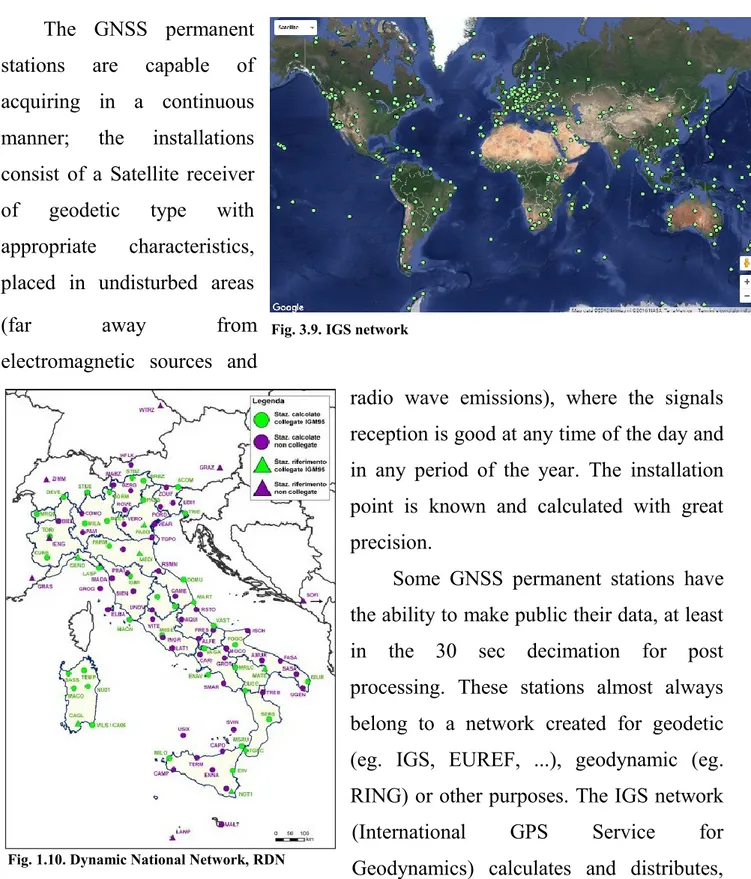
3.2.2. GNNS permanent stations The GNSS permanent stations are capable of acquiring in a continuous manner; the installations consist of a Satellite receiver of geodetic type with appropriate characteristics, placed in undisturbed areas
(far away from
electromagnetic sources and
radio wave emissions), where the signals reception is good at any time of the day and in any period of the year. The installation point is known and calculated with great precision.
Some GNSS permanent stations have the ability to make public their data, at least in the 30 sec decimation for post processing. These stations almost always belong to a network created for geodetic (eg. IGS, EUREF, ...), geodynamic (eg. RING) or other purposes. The IGS network (International GPS Service for Geodynamics) calculates and distributes,
Fig. 3.9. IGS network
3.2.2. GNNS permanent stations Chapter III
36
for scientific applications, i) the precise ephemeris of GPS and GLONASS satellites, ii) the parameters of the Earth's
rotation, iii) the corrections of the GNSS satellite clocks, iv) the coordinates and velocities of the ITRF stations ( International Terrestrial Reference Frame), v) the tropospheric and ionospheric information and vi) a series of information on the satellites (constellations, time series of the networks and the subnets calculated by various analysis centers (AC)).
The IGS network at present includes more than 350 stations
around the world (Fig. 3.9), managed by different authorities and with different monumentations. Their stations provide free rough data of precise orbits in ASCII files, with 30 sec acquisition rate and sp3 format.
RDN (National Dynamic Network) consists of 99 permanent GPS stations (Fig. 3.10) belonging to public authorities, they observe continuously the GNSS satellite signals and transmit them electronically to a Computing Center set up at the IGM Geodetic Service. The stations are evenly distributed throughout the national territory, with an average spacing of 100-150 km. In the network are included all stations on the national territory, already calculated in ITRS and IGS international networks.
RING (National Integrated Network GPS) is a network of about 140 permanent stations located on the national territory (Fig. 3.11), managed by INGV. The data with 30 sec acquisition rate, are available to the public on FTP, with daily files in RINEX format.
3.2.2. GNNS permanent stations Chapter III
37
NetGEO is a network consisting of 200 GNSS permanent stations realized by Geotop, equipped with GPS + GLONASS receivers. The receivers continuously acquire the signals emitted by visible satellites and transmit them to a control center that processes data, from all stations of the network, to make them available to users in Rinex format, with acquisition frequency of 1 sec. NetGeo is geo-referenced in the ETRF2000-RDN reference system, defined by IGM.
4.0. Basic SAR principles Chapter IV
38
Chapter IV
4.0. Basic SAR principles
In Remote Sensing scenarios the Synthetic Aperture Radar (SAR) sensor plays a significant role. It is a coherent active microwave remote sensing system which permits to generate high spatial resolution imageries, independently from weather conditions and during both day and night time by operating in the microwave spectrum region. SAR sensors have been largely employed to monitor the Earth surface.
A radar system is formed by a transmitting antenna that illuminates the surrounding space with electromagnetic waves. The transmitted energy is partially absorbed by the Earth's surface and partially scattered in all directions. A portion of the incident radiation is scattered back to the antenna, that is also equipped for the reception.
A radar system after an accurate measure of the time delay between the transmitted and the received echoes, knowing that the pulse travels at the speed of light, is able to figure out the distance (called slant range) between the sensor position, along its flight direction, and the illuminated targets on the ground.
The antenna directivity (the selectivity in the lighting the surrounding space) used for transmitting and receiving the radar signal enables the location of the object along the other dimension (called azimuth) (Fig. 4.1)