Titolo
Pre-test analysis of thermal-hydraulic behaviour of the NACIE facility for the
characterization of a fuel pin bundle
Ente emittente CIRTEN
PAGINA DI GUARDIA
Descrittori
Tipologia del documento: Collocazione contrattuale:
Rapporto Tecnico
Accordo di programma ENEA-MSE: tema di ricerca "Nuovo
nucleare da fissione" Generation IV Reactors
Termoidraulica dei metalli liquidi
Argomenti trattati:
Sommario
This report, carri ed out at the DIMNP (Dipartimento di Ingegneria Meccanica, Nucleare e della Produzione) of the University of Pisa in collaboration with ENEA Brasimone Research Centre, illustrates the pre-test thermo-fluidynamic analysis of the NAC[E (Natural Circulation Experiment) facility, built at ENEA, in its new configuration of the heat exchanger and of theheater system.
[n particular, the first part of the work regards the study performed by RELAP5/Mod3.3 system code, modified in order to take into account LBE fluid properties and the appropriate convective heat transfer correlations. The code was emp!oyed to support the design of SEARCH experimental campaign, devoted to characterize the performance of a wire spaced fue! bundle relevant for MYRRHA facility (i.e. heat exchange and pressure drop) inshutdown conditions and providing data for code validation. For this purpose, low heat power simulations on NAC[E facility have been performed to investigate the estab!ished loop natura! flow rate andrelated parameters for increasing values of loop hydraulic resistance. The second part of the work concems the first application, to a simplified representation of NACIE facility, of the coupling between the RELAP5 thermal-hydrau!ic system code and the CFD Fluent commerciaI code. Preliminary comparative analysis among the simulations performed by RELAP5-Fluent coupled codes and by RELAP5 stand-alone code showed very good agreement among them, giving confidence to this innovative coupling strategy..
Note: PAR2011 LP3-C3.C. Autori:
G. Barone, N. Forgione, D.Martelli (UNIPI) A. Del Nevo (ENEA)
Copia n. In carico a: NOME 2 FIRMA NOME 1 FIRMA
o
EMISSIONE 18/09/2011..r--_N_OM_E_-+- NA +-_M.-;II-..
1.
4
-n
/i:d".~!lA~~
ln:-o--+ NA --lA
/;
t
N
FIRMA
Pre-test analysis
of thermal-hydraulic behaviour of the NACIE facility
for the characterization of a fuel pin bundle
(Analisi numerica di pre-test
del comportamento termoidraulico dell’impianto NACIE
per la caratterizzazione di un fuel pin bundle)
G. Barone, N. Forgione, D. Martelli
(DIMNP – Università di Pisa)
A. Del Nevo
(ENEA – Brasimone)
Pisa, August 2012
Lavoro svolto in esecuzione dell’Attività LP3-C4
AdP MSE-ENEA sulla Ricerca di Sistema Elettrico - Piano Annuale di Realizzazione 2011 Progetto 1.3.1 “Nuovo Nucleare da Fissione:
2
Index
Summary ... .3
1. The NACIE facility ... 4
1.1 Heat source ... 5
1.2 Heat exchanger ... 6
2. Thermal-hydraulic pre-test analysis ... 8
2.1 RELAP5 NACIE model ... 8
2.2 Simulations description and boundary conditions ... 10
2.3 Simulation results and discussion ... 10
2.3.1 Natural circulation (Test NAT) ... 10
2.3.2 Natural circulation with additional flow resistance (Test VAL) ... 23
3. Analysis performed by RELAP5-Fluent coupled codes ... 32
3.1 RELAP5 and Fluent models ... 32
3.2 Coupling procedure... 35
3.3 Matrix of simulations ... 36
3.4 Obtained results ... 37
3.4.1 Natural circulation tests ... 37
3.4.2 Assisted circulation tests ... 44
3.4.3 ULOF test ... 50
4. Conclusions ... 53
References ... 54
Nomenclature ... 55
Appendix A ... 57
3
Summary
This report, carried out at the DIMNP (Dipartimento di Ingegneria Meccanica, Nucleare e della Produzione) of the University of Pisa in collaboration with ENEA Brasimone Research Centre, illustrates the pre-test thermo-fluidynamic analysis of the NACIE (Natural Circulation Experiment) facility, built at ENEA, in its new configuration of the heat exchanger and of the heater system.
In particular, the first part of the work regards the study performed by RELAP5/Mod3.3 system code, modified in order to take into account LBE fluid properties and the appropriate convective heat transfer correlations. The code was employed to support the design of SEARCH experimental campaign, devoted to characterize the performance of a wire spaced fuel bundle relevant for MYRRHA facility (i.e. heat exchange and pressure drop) in shutdown conditions and providing data for code validation. For this purpose, low heat power simulations on NACIE facility have been performed to investigate the established loop natural flow rate and related parameters for increasing values of loop hydraulic resistance. The second part of the work concerns the first application, to a simplified representation of NACIE facility, of the coupling between the RELAP5 thermal-hydraulic system code and the CFD Fluent commercial code. Preliminary comparative analysis among the simulations performed by RELAP5-Fluent coupled codes and by RELAP5 stand-alone code showed very good agreement among them, giving confidence to this innovative coupling strategy.
4
1. The NACIE facility
NACIE [1] is a loop facility designed at ENEA-Brasimone Research Centre, to qualify and characterize components, systems and procedures relevant for HLM nuclear technologies. In particular it is possible to carry out natural circulation and mixed convection experimental tests in the field of thermal hydraulic, fluid dynamics, chemistry control, corrosion and liquid metal heat exchange allowing the investigation of essential correlation for the design and development of new generation nuclear facilities. NACIE is a rectangular loop (7.5 m height) that basically consists of two vertical pipes (O.D. 2.5”, S40) (i.e. the downcomer and the riser), connected with two horizontal pipes (O.D. 2.5”, S40). A heat source (HS) (electric pins) is placed at the lower part of the riser, whereas a heat exchanger (HX) is placed on the downcomer side (a different height from the HS midplane could be configured). NACIE loop is entirely made of austenitic stainless steel, AISI 304, and can operate with both lead-bismuth (LBE) and lead as working fluid. The experimental tests will be carried out using LBE. A gas (argon) is injected through the riser during the assisted circulation tests to promote the circulation inside the loop.
Figure 1.1: NACIE facility conceptual sketch.
An expansion vessel is installed, coaxially with the riser (on the top part), which enables the thermal expansion of the LBE during operational transient and allows the separation and recovery of the argon from the LBE to be reused in a closed loop to promote liquid metal circulation. The free level of the expansion vessel is kept at a slight overpressure (about 200 mbar) by means of a hydrogen-argon mixture. The facility internal volume is about 0.1 m3 (100 liters), which totally corresponds to 1000 kg of liquid metal. The design temperature of the facility is 550°C even though it’s generally operated at a lower temperature.
7.5 m
5
Furthermore a ball valve will be installed to regulate the hydraulic losses. A conceptual scheme of NACIE with the main dimension is depicted in Figure 1.1.
1.1 Heat source
A specifically designed new heat source (HS) will be installed in the NACIE facility to carry out the experimental SEARCH WP2 campaign. The heat source [2] characterized by an overall thermal power of 250 kW; consists of 19 electrically heated pin bundle arranged in a hexagonal array and closed into a hexagonal wrapper as depicted in Figure 1.2.
Figure 1.2: Electrical wire-spaced pin bundle cross section.
The technical specifications are summarized in Table 1.1.
Table 1.1: Electrical wire-spaced pin bundle parameters.
d 6.55 mm Rod diameter
p/d 1.276 Pitch to diameter ratio
dw 1.75 mm Wire diameter
Hw 262 mm Wire pitch
q”max 1 MW/m2 Maximum heat flux at pin wall Qmax ~ 235 kW Maximum bundle thermal power
The electric pin (total length Ltot=2000 mm), shown in Figure 1.3, is characterized by an active region of L2 = 600 mm. No spacer grids are foreseen for the bundle, instead wire spacers will be installed over a pin length of approximately 1300 mm:
- L1 ~ 500 mm (Inactive) - L2 = 600 mm (Active) - L3 = 100 mm (Inactive)
6
Figure 1.3: Wire installation along pin length.
Pins 2, 4, 6, 7, 9, 16, 18 and 19 will be equipped with embedded thermocouples on a generatrix parallel to the pin axis, as shown in Figure 1.4. Three different levels will be considered z = 38, 300 and 562 mm starting from the beginning of the active region.
Figure1.4: Wall Embedded TCs location.
1.2 Heat exchanger
In order to remove the heat power from the new electrical bundle, a convenient “shell and tube” heat exchanger has been proposed (see Figure 1.5) [2]. Heat exchanger pipe parameters are found in Table 1.2. The tubes are arranged in a hexagonal lattice (one central and six surrounding tubes) and are double-wall type, in order to mitigate the axial thermal stresses caused by the differential thermal expansion and to avoid accidental contact of the liquid metal with water. The gap between the two walls (2.5 mm) is filled by steel powder (good thermal conductivity) to guarantee the thermal flux towards secondary water. Hot liquid metal flows downward through the inner pipes and exits from the bottom heat exchanger outlet. The shell side (where secondary sub-cooled water flows at a pressure of 16 bar) of the heat exchanger is divided into two separate sections:
- HX-2: Low power section ( 0.3 m) - HX-1: High power section (2.1 m)
7
Table 1.2: Heat Exchanger pipe geometrical parameters.
Component Pipe size Sch. de di t Material
[in] [mm] [mm] [mm]
Shell 16 40 406.4 381.0 12.7 AISI 316L
Inner tube 2 ½ 40 73.0 62.7 5.2 AISI 316L
Outer tube 3 40 88.9 77.9 5.5 AISI 316L
Each Section is associated with an independent secondary water loop which is activated according to the power that needs to be exchanged. Inside the high power section water flows counter-flow, while inside the low pressure section water flows cross-flow. The experimental tests discussed in this work will all be interested by the low power section HX-2 (10-35 kW), with a water flow rate of 10 m3/h and inlet temperature ranging from 120 to 170°C.
Figure 1.5: Heat Exchanger sections HX-2 and HX-1.
HX-2
HX-1
8
2 Thermal-hydraulic pre-test analysis
2.1 RELAP5 NACIE model
The system code RELAP5/Mod3.3 [3], modified to take into account LBE properties [4], has been used to generate NACIE model (see Figure 2.1), according to the facility experimental setup previously described.
9
Figure 2.1 shows the nodalizations of the primary LBE loop and of the two water secondary systems coupled with sections HX-1 and HX-2 respectively of the Heat Exchanger. Referring to this scheme, liquid metal circulates anticlockwise through the loop; LBE is heated in Pipe-110 (Heat Source) positioned at the bottom of the loop and is cooled through the heat exchanger (top of loop) modelled by Pipe-186 (HX-2 low power section ) and Pipe-190 (HX-1 high power section). According to the power to be exchanged, HX-1 or HX-2 is activated. The present report supports the design of SEARCH experimental campaign, devoted to characterizing the performance of MYRRHA fuel bundle (i.e. heat exchange and pressure drop) in shutdown conditions and to providing data for code validation. This experimental program is based on low power tests, therefore LBE exchanges power exclusively in heat section HX-2, water secondary loop associated to HX-1 being deactivated. NACIE gas assisted circulation has been modelled by mean of a time dependent junction (Tmdpjun-405) which injects the desired Aargon flow rate (Branch-125, riser bottom). argon reaches the top of the expansion vessel through the riser, enhancing liquid metal circulation. From the riser prolongation inside the expansion vessel (Pipe-146 and Pipe-148), LBE exits (in Branch-150) and is forced to pass downwards through the expansion vessel annular zone (Annulus-152 and Annulus-156) promoting, therefore, gas separation and avoiding argon from reaching the upper portion of the loop (namely Pipe-160 and Pipe-170). Only natural circulation tests are simulated in this work, consequently the argon injection has been deactivated. Liquid metal from the upper horizontal branch, goes downwards through Pipe-180 to the heat exchanger sections, HX-2 and HX-1. Height of HX-2 186) and HX-1 (Pipe-190) has been fixed to 0.3 m and 2.2 m respectively with a pipe cell’s length of 0.05 m. The two sections are thermally coupled with two independent systems, simulating the HX-2 and HX-1 water secondary side (Pipe-686 and Pipe-590). The two secondary systems are activated by means of time dependent junctions (Tmdpjun-615 and Tmdpjun-515) regulating the water mass flow rate. Only HX-2 secondary side water will be activated in these tests. LBE, exiting the heat exchanger sections, flows through the downcomer (Pipe-200 and Pipe-206) to the lower horizontal pipe of the loop (Pipe-210) to reach the lower Heat Source inactive portion (Pipe-100). A Motor valve (Mtrvlv-203) is inserted in the downcomer lower section (between Pipe-200 and Pipe 206) simulating the ball valve installed to regulate hydraulic losses. The nodalization is characterized by cells length of 0.1 m (mainly) for piping components and 5 cm for “heat-components” (namely Heat Source and the two Heat Exchanger sections). The value of the pipe’s wall roughness has been assumed ε=32 μm .
Electrical pin bundle Heat Source, has been modelled as follows: - Lower inactive portion (500 mm): Pipe-100;
- Active portion (600 mm): Pipe-110;
- Upper inactive portion (100 mm): Pipe-120, (first cell).
The pin bundle section is characterized by a flow area of 6.54∙10-4 m2 and by a hydraulic diameter of 4.14 10-3 m. The pressure losses caused by the wire-spaced pin bundle (for a total length of ~1.3 m) are taken into account introducing a pipe junction form loss coefficient, K, which is a function of the Reynolds number, Re, and can generally be expressed as:
K=A+B∙(Re)-C
where A, B and C are user-specified coefficient which have been derived from the Rehme equation [5] valid for wire spaced pin bundle (see Appendix A). Pressure losses associated with the bundle are dominant compared to the total ones; hence an accurate evaluation of the form coefficient, K, in this section of the loop, is an important issue for an adequate code flow prediction. Power Source, simulating the 19 fuel pins of the bundle (d=6.55mm, p/d=1.28), is modelled by an appropriate RELAP5 heat structure coupled with Pipe-110 (HS). Power is generated uniformly along 12 axial heat structures and released to the liquid metal, according to the convective vertical bundle option. For the Heat Exchanger (HX-1 and HX-2), heat structures are introduced to simulate power transfer from LBE (flowing within tubes), to cooling water flowing within the two secondary systems. Double wall AISI 316L tubes with steel powder inside their gap have been modelled (mean value of the conductivity, k~3 W/(mK)). Inside HX-1 (high power section) LBE exchange
10
power in counter-flow; the vertical bundle without crossflow option has been set for convective heat transfer water side (outside the tubes). In the low power section, HX-2, heat transfer occurs in crossflow mode and the value of the convective heat transfer coefficient has been fixed to 4600 W/(m2 K) resulting from CFD simulations.
2.2 Simulation description and boundary conditions
The total amount of liquid metal filling NACIE primary loop is around 1370 kg of LBE at an initial temperature of 283°C (563.15 K). LBE initial level is set about half way of expansion vessel’s height (Branch-150), 16 cm above the riser outlet. argon pressure inside the expansion vessel has been set to 1.2∙105 Pa. Heat exchanger has been placed at the top of the downcomer to enhance LBE natural circulation with a thermal center elevation (vertical distance between HX-2 and HS mid-planes) fixed to 6.25 m. Secondary side of the low power heat exchanger (HX-2) is characterized by a pressure of 16 bar and water flow rate is set to 10 m3/h. The heat transfer coefficient of water flowing cross-flow through HX-2 has been estimated from CFD simulations and fixed to the value of hw= 4600 W/(m2K). All RELAP5 simulations have been performed with the boundary conditions described above. No heat dispersion towards external environment has been considered. Simulations aim to investigate safety related parameters in case of a natural circulation condition for different values of the mass flow rate. Three power levels of the Heat Source have been investigated:
- Q1=10.8 kW - Q2=21.7 kW - Q3=32.5 kW
The reference heat flux value at the wall of ~1 MW/m2 is obtained for bundle nominal power of ~ 235 kW. The effect of HX-2 water inlet temperature, in the range of 120-170°C, has been investigated as well. Heat Source power is switched on after 2000 s from the beginning of each simulation; at the same time secondary water starts flowing through HX-2 secondary loop. Two sets of simulations have been executed: - Test NAT, which is aimed at characterizing the performance of the loop and the LBE mass flow rate in
natural circulation conditions, for the three reference power level.
- Test VAL, which is devoted to evaluating the system’s performance, for different additional loop hydraulic resistances (by means of a valve, Mtrvlv-203), that progressively reduce natural circulation mass flow rate obtained in Test NAT.
2.3 Simulations results and discussion
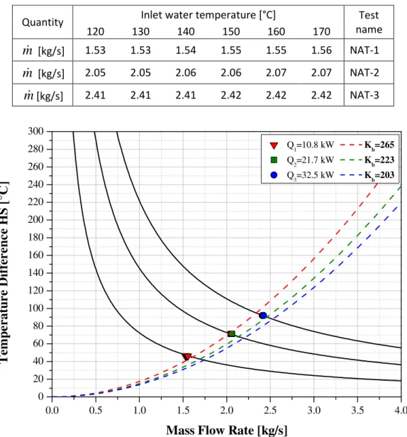
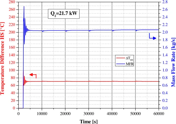
2.3.1 Natural circulation (Test NAT)The first series of simulations (Test NAT) aim at investigating the above described NACIE loop behaviour under natural circulation conditions, for three reference power levels (Q1=10.8 kW, Q2=21.7 kW and Q3=32.5 kW). As described before, HS and HX-2 thermal center distance has been set at 6.25 m. During these simulations it can be assumed that the NACIE loop losses of pressure are predominantly caused by the wire-spaced bundle section. Moreover, in each simulation of Test NAT, named NAT-1, NAT-2 and NAT-3 (according to the heat power level), the influence of the inlet HX-2 secondary water temperature, Tw, has been investigated performing a stepwise increase of the secondary water, from 120 up to 170°C (step of 10°C). The time span for each water temperature level is 10000 s, (to allow the achievement of stationary conditions) for total simulation duration of 60000 s. Table 2.1 summarizes the estimated LBE mass flow rate, for each simulation, expected in NACIE loop. These values are obtained at the end of the time span when the system has reached “quasi” steady state condition.
11
Table 2.1: Natural circulation mass flow rate driven through NACIE loop.
Quantity Inlet water temperature [°C] Test
name
120 130 140 150 160 170
m
&
[kg/s] 1.53 1.53 1.54 1.55 1.55 1.56 NAT-1m
&
[kg/s] 2.05 2.05 2.06 2.06 2.07 2.07 NAT-2m
&
[kg/s] 2.41 2.41 2.41 2.42 2.42 2.42 NAT-3Figure 2.2: HS temperature difference versus LBE natural flow rate: RELAP5 simulated results and the related simplified thermal hydraulic model estimations (dash-lines).
Simulation results show that water temperature, Tw, has a negligible influence on the value of the LBE mass flow rate established in NACIE loop. These results are depicted in Figure 2.2 which plots the obtained values of natural mass flow rate, m& , versus the corresponding bundle temperature difference, ΔTHS, for the reference power levels. According to the power level, Q, results stays on three curves generated from the following balance equation:
HS p Q T c m ∆ = ⋅ & (2.1)
The LBE specific heat capacity at constant pressure has been approximately set at c = 147 J/(kg K). p
Furthermore, by means of a simple balance between driving and resistance force, a simplified thermal-hydraulic model of NACIE loop in pure natural circulation can be written as:
2 ( ) 2 HS u g T H K u ρ β⋅ ∆ ⋅ = ⋅ ⋅ρ (2.2) 0.0 0.5 1.0 1.5 2.0 2.5 3.0 3.5 4.0 0 20 40 60 80 100 120 140 160 180 200 220 240 260 280 300
T
em
p
er
a
tu
re
D
if
fe
re
n
ce
H
S
[
°C
]
Mass Flow Rate [kg/s]
Q1=10.8 kW Kb=265
Q2=21.7 kW Kb=223
12
In the simplified assumption that K is not a function of u, i.e. for sufficiently high Reynolds number, it is possible to obtain in closed form a relationship between the temperature drop and the mass flow rate in the loop: 2 2 2 2 2 2 HS Ku K T m g Hβ g Hβ ρ A ∆ = = & (2.3) where,
K=Kb+Kl+Kv : total resistance coefficient associated to reference cross section A. Kb : bundle resistance coefficient.
Kl : loop resistance coefficient (related to pipe friction, bends, contractions, enlargements and expansion vessel).
Kv : valve resistance coefficient.
u : LBE velocity magnitude for the reference cross section A. A : reference cross section.
β : LBE volumetric thermal expansion coefficient. H : thermal centers elevation (H=6.25 m)
g : gravity acceleration
A comparison of the LBE mass flow rate derived using the simplified thermal hydraulic model and results obtained by RELAP5 simulations is illustrated in Figure 2.2 as well. The three thermodynamic model parabolic trends associated with reference power levels are characterized by different bundle resistance coefficients, Kb, which are derived from RELAP5 results (for Tw=170°C). The value of the loop resistance coefficient has been approximately set to a constant value of kl=15. Valve resistance coefficient is Kv=0, assuming the valve completely opened and the value of β and ρ have been taken for mean LBE temperature. A sufficient agreement could be observed although the thermal hydraulic model results are slightly higher compared to the ones obtained by the simulations. Detailed trend of LBE natural circulation mass flow rate and the related temperature difference through the inlet and outlet section of the HS, are shown, for each power level, in Figures 2.3(a,b,c).
Figure 2.3.a: LBE mass flow rate along NACIE loop and the related ∆THS ( Test NAT-1).
0 10000 20000 30000 40000 50000 60000 0 20 40 60 80 100 120 140 160 180 200 220 240 260 280
Q
1=10.8 kW
T
em
p
er
a
tu
re
D
if
fe
re
n
ce
H
S
[
°C
]
Time [s]
∆THS MFR 0.0 0.2 0.4 0.6 0.8 1.0 1.2 1.4 1.6 1.8 2.0 2.2 2.4 2.6 2.8M
a
ss
F
lo
w
R
a
te
[
k
g
/s
]
13
Figure 2.3.b: LBE mass flow rate along NACIE loop and the related ∆THS ( Test NAT-2).
Figure 2.3.c: LBE mass flow rate along NACIE loop and the related ∆THS (Test NAT-3).
0 10000 20000 30000 40000 50000 60000 0 20 40 60 80 100 120 140 160 180 200 220 240 260 280
Q
2=21.7 kW
T
em
p
er
a
tu
re
D
if
fe
re
n
ce
H
S
[
°C
]
Time [s]
∆THS MFR 0.0 0.2 0.4 0.6 0.8 1.0 1.2 1.4 1.6 1.8 2.0 2.2 2.4 2.6 2.8M
a
ss
F
lo
w
R
a
te
[
k
g
/s
]
0 10000 20000 30000 40000 50000 60000 0 20 40 60 80 100 120 140 160 180 200 220 240 260 280Q
3=32.5 kW
T
em
p
er
a
tu
re
D
if
fe
re
n
ce
H
S
[
°C
]
Time [s]
∆THS MFR 0.0 0.2 0.4 0.6 0.8 1.0 1.2 1.4 1.6 1.8 2.0 2.2 2.4 2.6 2.8M
a
ss
F
lo
w
R
a
te
[
k
g
/s
]
14
In Figures 2.4(a,b,c) the trends of the average LBE inlet and outlet Heat Source temperatures are plotted, together with pin surface temperatures estimated at the thermocouples location (see Figure 1.4). The considered heights for the TCs along the bundle active length (Lact = 600) are:
- z = 38 mm (TCd) - z = 300 mm (TCm) - z = 562 mm (TCu)
Results are summarized in Table 2.2. The stepwise increasing trend of the HX-2 water inlet temperature is depicted as well. Results show how the loop’s mean temperature increases with the power level; moreover, increasing water inlet temperature causes a further increase in the loop’s mean temperature trend and consequently a higher value of the maximum LBE temperature and clad surface temperature (TCu). For Q3=32.5 kW (Test NAT-3) and Tw=170°C, in maximum temperature conditions, the previously mentioned temperatures remain below 431°C. Furthermore, the minimum LBE temperature (176°C) is observed for Q1=10.8 kW (Test NAT-1) and Tw=120°C, with a safety margin of about 50°C from LBE freezing point (124°C).
Figure 2.4.a: Inlet and outlet LBE temperatures along HS, clad temperature at TCs locations and trend of the HX-2 water inlet temperature (Test NAT-1).
0 10000 20000 30000 40000 50000 60000 100 150 200 250 300 350 400 450
Q
1=10.8 kW
T
em
p
er
a
tu
re
[
°C
]
Time [s]
TCu HS_in TC m HS_out TC d Water_in15
Figure 2.4.b: Inlet and outlet LBE temperatures along HS, clad temperature at TCs locations and trend of the HX-2 water inlet temperature (Test NAT-2).
Figure 2.4.c: Inlet and outlet LBE temperatures along HS, clad temperature at TCs locations and trend of the HX-2 water inlet temperature (Test NAT-3).
0 10000 20000 30000 40000 50000 60000 100 150 200 250 300 350 400 450
Q
2=21.7 kW
T
em
p
er
a
tu
re
[
°C
]
Time [s]
TC u HS_in TCm HS_out TCd Water_in 0 10000 20000 30000 40000 50000 60000 100 150 200 250 300 350 400 450Q
3=32.5 kW
T
em
p
er
a
tu
re
[
°C
]
Time [s]
TCu HS_in TC m HS_out TC d Water_in16
Table 2.2: LBE inlet/outlet HS temperature and clad surface temperature at thermocouple locations [°C].
Temperature [°C]
Inlet water temperature Tw [°C] Test name 120 130 140 150 160 170 HS In 176 185 195 204 214 223 NAT-1 HS Out 223 232 241 250 260 269 TCd 184 193 202 212 221 230 TCm 204 213 222 232 241 250 TCu 224 233 243 252 261 271 HS In 228 237 246 255 264 272 NAT-2 HS Out 299 308 317 325 334 343 TCd 240 249 258 267 276 284 TCm 271 280 288 297 306 315 TCu 302 310 319 328 337 346 HS In 291 300 309 318 327 335 NAT-3 HS Out 383 392 401 410 419 427 TCd 307 317 325 334 343 351 TCm 347 356 365 374 383 391 TCu 387 396 405 414 423 431
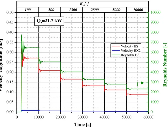
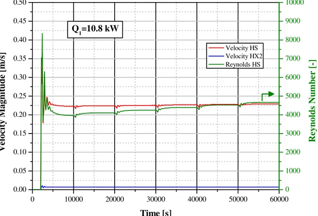
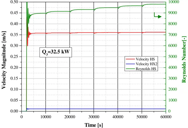
LBE velocity magnitude through the rod bundle Heat Source and inside the tubes of the low power Heat Exchanger (HX-2) are depicted in Figures 2.5(a,b,c), for the three reference power levels. An estimation of the Reynolds number trend is shown as well (right axis). Reynolds number has been evaluated for LBE mean properties (at HS half height). Concerning the LBE velocity magnitude through the HS, an analogous trend as for the mass flow rate can be observed and the velocity magnitude is not influenced by increasing water inlet temperature. HS velocity magnitude is about 0.23 m/s for test NAT-1, 0.30 m/s for test NAT-2 and 0.36 m/s for test NAT-3. LBE velocity magnitude inside the Heat Exchanger tubes is in the order of magnitude of some millimetres per seconds: 0.007 m/s for test NAT-1, 0.009 m/s for test NAT-2 and 0.011 m/s for test NAT-3.
Concerning the Reynolds number, it ranges (values for water temperature of 120 and 170°C): - from 3970 to 4670 (test NAT-1)
- from 6430 to 7240 (test NAT-2) - from 8970 to 9800 (test NAT-3)
Turbulent flow regime is established inside the bundle Heat Source for all the considered tests. An increase in Reynolds number is observed with the increasing inlet water temperature caused by the increase of the ratio (ρ/μ)LBE with the loop mean temperature.
17
Figure 2.5.a: LBE Velocity along the HS bundle and inside HX-2 tubes. Reynolds number for HS (Test NAT-1).
Figure 2.5.b: LBE Velocity along the HS bundle and inside HX-2 tubes. Reynolds number for HS (Test NAT-2)
0 10000 20000 30000 40000 50000 60000 0.00 0.05 0.10 0.15 0.20 0.25 0.30 0.35 0.40 0.45 0.50
Q
1=10.8 kW
V
el
o
ci
ty
M
a
g
n
it
u
d
e
[m
/s
]
Time [s]
Velocity HS Velocity HX2 Reynolds HS 0 1000 2000 3000 4000 5000 6000 7000 8000 9000 10000R
ey
n
o
ld
s
N
u
m
b
er
[
-]
0 10000 20000 30000 40000 50000 60000 0.00 0.05 0.10 0.15 0.20 0.25 0.30 0.35 0.40 0.45 0.50Q
2=21.7 kW
V
el
o
ci
ty
M
a
g
n
it
u
d
e
[m
/s
]
Time [s]
Velocity HS Velocity HX2 Reynolds HS 0 1000 2000 3000 4000 5000 6000 7000 8000 9000 10000R
ey
n
o
ld
s
N
u
m
b
er
[
-]
18
Figure 2.5.c: LBE Velocity along the HS bundle and inside HX-2 tubes. Reynolds number for HS (Test NAT-3).
LBE heat transfer coefficients (HTC) for HS (pin bundle) and for HX-2 (tube side) are depicted in Figures 2.6(a,b,c), for the three considered tests. The heat transfer coefficient water side is plotted as well. It is set from CFD simulations to the value of 4600 W/(m2 K). Vertical bundle heat transfer coefficient is evaluated by RELAP5, according to Ushakov correlation [6], while for LBE flowing tube side through the heat exchanger, Seban [7] relation is used. Obtained results are summarized in Table 2.3.
Table 2.3: LBE heat transfer coefficient [W/(m2K)], for HS (bundle) and HX-2 (tube side). HTC
[W/(m2K)]
Inlet water temperature [°C] Test
name 120 130 140 150 160 170 HS 17458 17682 17915 18145 18373 18598 NAT-1 HX-2 949 961 975 988 1001 1014 HS 19 756 19 966 20 174 20 380 20 584 20 786 NAT-2 HX-2 1 063 1 075 1 087 1 099 1 110 1 122 HS 21926 22128 22312 22508 22703 22866 NAT-3 HX-2 1182 1193 1204 1215 1227 1236
A slight heat transfer coefficient increase is observed with inlet water temperature; while from simulation NAT-1 to simulation NAT-3, HTC increases by about 20%.
0 10000 20000 30000 40000 50000 60000 0.00 0.05 0.10 0.15 0.20 0.25 0.30 0.35 0.40 0.45 0.50
Q
3=32.5 kW
V
e
lo
c
it
y
M
a
g
n
it
u
d
e
[
m
/s
]
Time [s]
Velocity HS Velocity HX2 Reynolds HS 0 1000 2000 3000 4000 5000 6000 7000 8000 9000 10000R
e
y
n
o
ld
s
N
u
m
b
e
r[
-]
19
Figure 2.6.a: Heat transfer coefficient for LBE and water (Test NAT-1).
Figure 2.6.b: Heat transfer coefficient for LBE and water (Test NAT-2).
0 10000 20000 30000 40000 50000 60000 5000 10000 15000 20000 25000
Q
1=10.8 kW
H
ea
t
T
ra
n
sf
er
C
o
ef
fi
ci
en
t
[W
/(
m
2K
)]
Time [s]
HS (Ushakov) HX2_LBE HX2_Water 0 10000 20000 30000 40000 50000 60000 5000 10000 15000 20000 25000Q
2=21.7 kW
H
e
a
t
T
r
a
n
sf
e
r
C
o
ef
fi
ci
e
n
t
[W
/(
m
2K
)]
Time [s]
HS (Ushakov) HX2_LBE HX2_Water20
Figure 2.6.c: Heat transfer coefficient for LBE and water (Test NAT-3).
The pressure loss resistance coefficient, Kb, has been set in NACIE input, introducing coefficients in the bundle junctions form loss card, in order to obtain an equivalent loss coefficient, according to Rehme correlation (see Eq. A.4 in Appendix A). The value of Kb from RELAP5 has been compared to the theoretical value calculated with Rehme correlation, KR, for wire spaced fuel bundle. As depicted in Figure 2.7(a,b,c) the two different evaluations are coincident. In the same figures, the value of the bundle pressure losses, ΔPb, estimated using Eq.2.5, is compared to the theoretical pressure loss, ∆PR, obtained using KR value in the following correlation:
2 1 2 R R b ref P K ρ u ∆ = ⋅ (2.4)
Where ρb is the mean value of LBE density inside the fuel bundle and uref is the loop reference velocity. The ΔPb has been estimated subtracting the pressure head to the bundle absolute pressure difference according to the following correlation:
1 ( ) b N b in out i i i P P P g hρ = ∆ = − − ⋅
∑
(2.5)Where, Pin and Pout are the bundle absolute inlet and outlet pressure, hi is the height of the RELAP5 bundle pipe hydrodynamic sub-volumes, Nb is the number of sub-volumes, ρi is the LBE density of the sub-volume and g is the gravity acceleration. Results show sufficient agreement with the theoretical estimation, being about 3 % lower for all three simulations. Table 2.4 summarizes the values of Kb and bundle pressure losses ΔPb evaluated with Eq. 2.5. Resistance coefficient slightly decreases with temperature due to Reynolds number increase (increase of LBE ρ/μ ratio) which causes a decrease of Darcy-Weisbach friction factor, fR, in Rehme correlation (see Eq. A.2 in Appendix A). Consequently a slight decrease of bundle pressure loss is observed. 0 10000 20000 30000 40000 50000 60000 5000 10000 15000 20000 25000
Q
3=32.5 kW
H
ea
t
T
ra
n
sf
er
C
o
ef
fi
ci
en
t
[W
/(
m
2K
)]
Time [s]
HS (Ushakov) HX2_LBE HX2_Water21
Table 2.4: Resistance coefficient Kb and pressure drop ΔPb [Pa] along the bundle.
Quantity Inlet water temperature [°C] Test
name 120 130 140 150 160 170 Kb [-] 285 280 276 272 268 265 NAT-1 ΔPb [Pa] 3476 3451 3430 3410 3391 3374 Kb [-] 235 233 231 228 226 225 NAT-2 ΔPb [Pa] 5138 5117 5097 5079 5061 5044 Kb [-] 210 208 207 206 204 203 NAT-3 ΔPb [Pa] 6372 6354 6337 6319 6301 6292
Figure 2.7.a: Bundle resistance coefficient and pressure drop (Test NAT-1).
0 10000 20000 30000 40000 50000 60000 0 50 100 150 200 250 300 350 400 450 500
K
B
u
n
d
le
[
-]
Time [s]
K (RELAP5) K (Rehme) ∆P (Bundle) ∆P (Rehme)Q
1=10.8 kW
0 1000 2000 3000 4000 5000 6000 7000 8000 9000 10000 ∆∆∆∆P
B
u
n
d
le
[
P
a
]
22
Figure 2.7.b: Bundle resistance coefficient and pressure drop (Test NAT-2).
Figure 2.7.c: Bundle resistance coefficient and pressure drop (Test NAT-3).
0 10000 20000 30000 40000 50000 60000 0 50 100 150 200 250 300 350 400 450 500
K
B
u
n
d
le
[
-]
Time [s]
K (RELAP5) K (Rehme) ∆P (Bundle) ∆P (Rehme) 0 1000 2000 3000 4000 5000 6000 7000 8000 9000 10000 ∆∆∆∆P
B
u
n
d
le
[
P
a
]
Q
2=21.7 kW
0 10000 20000 30000 40000 50000 60000 0 50 100 150 200 250 300 350 400 450 500K
B
u
n
d
le
[
-]
Time [s]
K (RELAP5) K (Rehme) ∆P (Bundle) ∆P (Rehme) 0 1000 2000 3000 4000 5000 6000 7000 8000 9000 10000 ∆∆∆∆P
B
u
n
d
le
[
P
a
]
Q
3=32.5 kW
23
2.3.2 Natural circulation with additional flow resistance (Test VAL)
The second series of simulations (Test VAL) aims at investigating NACIE behaviour in case of reduced natural circulation flow rate caused by an additional hydraulic resistance through the loop. Therefore, Test VAL has been performed by progressively closing the valve represented in NACIE RELAP5 model (see Figure 2.1) by the component Mtrvlv-203. Valve area is reduced with a stepwise trend in order to reach six progressively higher resistance coefficients: Kv=100, 500, 1300, 2800, 5000, 10000. RELAP5 dependence of Kv upon valve area is discussed in Appendix A. The time span for each value of Kv has been fixed to 10000 seconds in order for the loop parameters to reach stationary conditions. Inlet water temperature in the heat exchanger HX-2 has been fixed to Tw=170°C. Simulation results are summarized in Figure 2.8, which show, for each power level Q1=10.8 kW, Q2=21.7 kW and Q3=32.5 kW, LBE mass flow rate for progressive Kv increase (from Kv=0 of test NAT to Kv =10000) and the associated HS temperature difference. The curves based upon the simplified thermal hydraulic model introduced previously are depicted on the same plot. The value of resistance coefficient in Eq. 2.3 (K=Kb+Kv+Kl ) has been evaluated considering the Kb value for the intermediate power level simulation VAL-2, Kl=15 and Kv the valve resistance coefficient.
Figure 2.8: HS temperature difference versus LBE natural flow rate: RELAP5 simulation results for increasing values of Kv and the related simplified thermal hydraulic model estimations (dash-lines) Outcomes show a sufficient agreement of RELAP5 results with the ones estimated by the simplified thermal hydraulic model for high values of the valve resistance coefficient, while for lower Kv the model provides slightly higher values of the LBE mass flow rate as observed for test NAT. Table 2.5 summarizes stationary LBE mass flow rate values obtained from RELAP5 simulation at increasing Kv, for the three power levels. 0.0 0.5 1.0 1.5 2.0 2.5 3.0 3.5 4.0 0 50 100 150 200 250 300 350 400 kv=0 kv=100 kv=500 kv=1300 kv=2800 kv=5000
T
em
p
er
a
tu
re
D
if
fe
re
n
ce
H
S
[
°C
]
Mass Flow Rate [kg/s]
Q1=10.8 kW
Q2=21.7 kW
Q3=32.5 kW
24
Table 2.5: LBE flow rate for the reference valve resistance coefficient.
Quantity Valve resistance coefficient Kv [-] Test
name
0 100 500 1300 2800 5000 10000
m
&
[kg/s] 1.56 1.39 1.10 0.87 0.70 0.59 0.47 VAL-1m
&
[kg/s] 2.07 1.83 1.41 1.11 0.89 0.75 0.60 VAL-2m
&
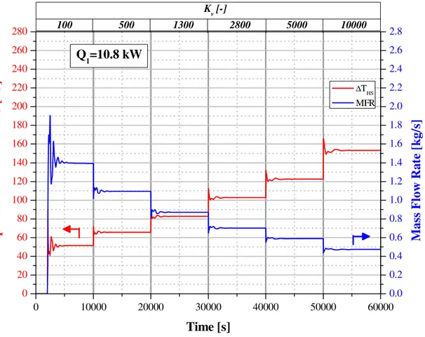
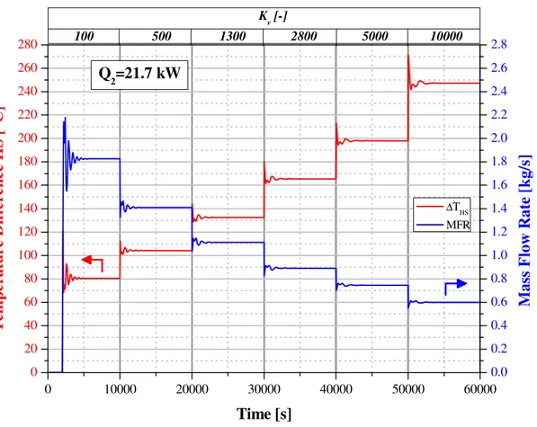
[kg/s] 2.42 2.12 1.62 1.27 1.02 0.85 0.68 VAL-3In Figures 2.9(a,b,c) the trends of LBE flow rate and HS temperature difference are reported for each power level with the increase of Kv value (case Tw=170°C).
Figure 2.9.a: LBE mass flow rate along NACIE loop and the related ∆THS (Test VAL-1).
0 10000 20000 30000 40000 50000 60000 0 20 40 60 80 100 120 140 160 180 200 220 240 260 280
Q
1=10.8 kW
Kv [-] 100 500 1300 2800 5000 10000T
e
m
p
er
a
tu
r
e
D
if
fe
r
e
n
c
e
H
S
[
°C
]
Time [s]
∆THS MFR 0.0 0.2 0.4 0.6 0.8 1.0 1.2 1.4 1.6 1.8 2.0 2.2 2.4 2.6 2.8M
a
ss
F
lo
w
R
a
te
[
k
g
/s
]
25
Figure 2.9.b: LBE mass flow rate along NACIE loop and the related ∆THS (Test VAL-2).
Figure 2.9.c: LBE mass flow rate along NACIE loop and the related ∆THS, (Test VAL-3).
0 10000 20000 30000 40000 50000 60000 0 20 40 60 80 100 120 140 160 180 200 220 240 260 280 Q 2=21.7 kW Kv [-] 100 500 1300 2800 5000 10000 T em p e ra tu r e D if fe re n c e H S [ °C ] Time [s] ∆THS MFR 0.0 0.2 0.4 0.6 0.8 1.0 1.2 1.4 1.6 1.8 2.0 2.2 2.4 2.6 2.8 M a ss F lo w R a te [ k g /s ] 0 10000 20000 30000 40000 50000 60000 0 20 40 60 80 100 120 140 160 180 200 220 240 260 280 300 320 340 360 Q3=32.5 kW Kv [-] 100 500 1300 2800 5000 10000 T e m p er a tu r e D if fe r e n ce H S [ °C ] Time [s] ∆THS MFR 0.0 0.2 0.4 0.6 0.8 1.0 1.2 1.4 1.6 1.8 2.0 2.2 2.4 2.6 2.8 3.0 3.2 3.4 3.6 M a ss F lo w R a te [ k g /s ]
26
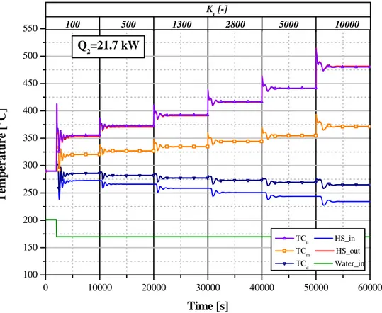
LBE temperature for HS inlet/outlet and pin surface temperatures for the TCs position (see Figures 1.4) are depicted in Figure 2.10(a, b, c). Table 2.6 summarizes the obtained results.
Table 2.6: Temperature of LBE HS inlet/outlet and of clad surface at TCs locations [°C]. Temp.
[°C]
Valve resistance coefficient Kv [-] Test name
100 500 1300 2800 5000 10000 HS in 222 217 213 208 204 201 VAL-1 HS out 273 283 296 311 327 355 TCd 230 227 224 222 220 220 TCm 252 255 260 266 273 286 TCu 274 284 296 311 327 354 HS in 273 266 259 251 244 234 VAL-2 HS out 353 370 391 416 442 481 TCd 286 282 277 273 269 265 TCm 320 327 334 344 355 371 TCu 356 372 392 417 442 480 HS in 330 320 308 297 288 273 VAL-3 HS out 435 457 483 517 551 602 TCd 348 341 333 327 322 314 TCm 393 400 409 422 435 455 TCu 439 460 486 518 551 601
Figure 2.10.a: Inlet and outlet LBE temperatures along HS, clad temperature at TCs locations (Test VAL-1).
0 10000 20000 30000 40000 50000 60000 100 150 200 250 300 350 400 450 500 550 Kv [-] 100 500 1300 2800 5000 10000
Q
1=10.8 kW
T
em
p
er
a
tu
re
[
°C
]
Time [s]
TCu HS_in TCm HS_out TCd Water_in27
Figure 2.10.b: Inlet and outlet LBE temperatures along HS, clad temperature at TCs locations (Test VAL-2).
Figure 2.10.c: Inlet and outlet LBE temperatures along HS, clad temperature at TCs locations (Test VAL-3).
0 10000 20000 30000 40000 50000 60000 100 150 200 250 300 350 400 450 500 550 Kv [-] 100 500 1300 2800 5000 10000 Q2=21.7 kW T e m p e ra tu re [ °C ] Time [s] TCu HS_in TCm HS_out TCd Water_in 0 10000 20000 30000 40000 50000 60000 100 150 200 250 300 350 400 450 500 550 600 650 Kv [-] 100 500 1300 2800 5000 10000 Q 3=32.5 kW T em p era tu re [ °C ] Time [s] TCu HS_in TCm HS_out TCd Water_in
28
Results show (case Tw=170°C) that for Test VAL-3 and Kv greater than 1300 the predicted clad temperature at the upper thermocouple location is above 500°C reaching the value of about 600°C for Kv=10000. For the same TCs location, test VAL-1 and VAL-2, give temperatures below 480°C at the maximum Kv. LBE velocity magnitude relative to Heat Source and to HX-2 (tube side) are summarized in Table 2.7 together with the value of the Reynolds number of the LBE flowing through the Heat Source bundle. Reynolds number has been evaluated at HS mid plane. Figures 2.11(a,b,c) show the trends of the above mentioned quantities for tests VAL-1, VAL2 and VAL-3.
Table 2.7: LBE Velocity magnitude [m/s] in Heat Source and HX-2; HS Reynolds number.
Quantity Valve resistance coefficient Kv [-] name Test
100 500 1300 2800 5000 10000 Vel. HS [m/s] 0.20 0.16 0.13 0.10 0.09 0.07 VAL-1 Vel. HX [m/s] 0.0062 0.0049 0.0039 0.0031 0.0026 0.0021 Rey HS [-] 4194 3322 2671 2184 1861 1540 Vel. HS [m/s] 0.27 0.21 0.16 0.13 0.11 0.09 VAL-2 Vel. HX [m/s] 0.008 0.006 0.005 0.004 0.003 0.003 Rey HS [-] 6462 5047 4032 3289 2805 2317 Vel. HS [m/s] 0.32 0.24 0.19 0.15 0.13 0.10 VAL-3 Vel. HX [m/s] 0.010 0.007 0.006 0.005 0.004 0.003 Rey HS [-] 8622 6655 5283 4301 3666 3020
Figure 2.11.a: LBE Velocity along HS bundle, inside HX-2 tubes and HS Reynolds number for the considered Kv (Test VAL-1).
Kv [-] 100 500 1300 2800 5000 10000 0 10000 20000 30000 40000 50000 60000 0.00 0.05 0.10 0.15 0.20 0.25 0.30 0.35 0.40 0.45 0.50 Q 1=10.8 kW V e lo ci ty M a g n it u d e [ m /s ] Time [s] Velocity HS Velocity HX2 Reynolds HS 0 1000 2000 3000 4000 5000 6000 7000 8000 9000 10000 R ey n o ld s N u m b er [ -]
29
Figure 2.11.b: LBE Velocity along HS bundle, inside HX-2 tubes and HS Reynolds number for the considered Kv (Test VAL-2).
Figure 2.11.c: LBE Velocity along HS bundle, inside HX-2 tubes and HS Reynolds number for the considered Kv (Test VAL-3).
K v [-] 100 500 1300 2800 5000 10000 0 10000 20000 30000 40000 50000 60000 0.00 0.05 0.10 0.15 0.20 0.25 0.30 0.35 0.40 0.45 0.50 Q 2=21.7 kW V el o ci ty M a g n it u d e [ m /s ] Time [s] Velocity HS Velocity HX2 Reynolds HS 0 1000 2000 3000 4000 5000 6000 7000 8000 9000 10000 R e y n o ld s N u m b e r [ -] Kv [-] 100 500 1300 2800 5000 10000 0 10000 20000 30000 40000 50000 60000 0.00 0.05 0.10 0.15 0.20 0.25 0.30 0.35 0.40 0.45 0.50 Q3=32.5 kW V e lo ci ty M a g n it u d e [ m /s ] Time [s] Velocity HS Velocity HX2 Reynolds HS 0 1000 2000 3000 4000 5000 6000 7000 8000 9000 10000 R e y n o ld s N u m b e r [ -]
30
The values of the bundle resistance coefficient, Kb, obtained by RELAP5, and the bundle pressure losses, ΔPb, estimated by Eq. 2.5 are reported in Table 2.8.
Table 2.8: Resistance coefficient Kb and pressure drop ΔPb [Pa] along the bundle.
Quantity Valve resistance coefficient Kv [-] Test
name 100 500 1300 2800 5000 10000 Kb [-] 277 310 348 391 433 493 VAL-1 ΔPb [Pa] 2848 1992 1436 1067 847 636 Kb [-] 234 259 288 320 350 395 VAL-2 ΔPb [Pa] 4121 2749 1918 1389 1081 803 Kb [-] 212 234 257 283 308 345 VAL-3 ΔPb [Pa] 5069 3290 2254 1608 1237 909
Figures 2.12(a,b,c) report the trends of Kb and ΔPb, for the considered valve resistance coefficient for test VAL-1, VAL-2 and VAL-3 (Tw=170°C).
Figure 2.12.a. Bundle resistance coefficient and pressure drop (Test VAL-1).
0 10000 20000 30000 40000 50000 60000 0 50 100 150 200 250 300 350 400 450 500 550 Kv [-] 100 500 1300 2800 5000 10000 Q 1=10.8 kW K B u n d le [ -] Time [s] K Bundle ∆P Bundle 0 1000 2000 3000 4000 5000 6000 7000 8000 9000 10000 11000 ∆∆∆∆ P B u n d le [ P a ]
31
Figure 2.12.b: Bundle resistance coefficient and pressure drop (Test VAL-2).
Figure 2.12.c: Bundle resistance coefficient and pressure drop (Test VAL-3).
0 10000 20000 30000 40000 50000 60000 0 50 100 150 200 250 300 350 400 450 500 550 Kv [-] 100 500 1300 2800 5000 10000 Q2=21.7 kW K B u n d le [ -] Time [s] K Bundle ∆P Bundle 0 1000 2000 3000 4000 5000 6000 7000 8000 9000 10000 11000 ∆∆∆∆ P B u n d le [ P a ] 0 10000 20000 30000 40000 50000 60000 0 50 100 150 200 250 300 350 400 450 500 550 Kv [-] 100 500 1300 2800 5000 10000 Q3=32.5 kW K B u n d le [ -] Time [s] K Bundle ∆P Bundle 0 1000 2000 3000 4000 5000 6000 7000 8000 9000 10000 11000 ∆∆∆∆ P B u n d le [ P a ]
32
3. Analysis performed by RELAP5-Fluent coupled codes
In this section the activity performed at the University of Pisa concerning the coupling between the RELAP5/Mod3.3 system code [3], modified to take into account the properties and heat transfer correlations to be used for the liquid lead and LBE [8-9], and the CFD Fluent code [10] is presented.
The set-up numerical model is based on a two-way semi-implicit coupling scheme and it has been preliminarily applied to NACIE facility in its new configuration (see section 1). In particular, the vertical part of the loop including the heater system and part of the piping before and after it has been simulated by the Fluent code in a simplified 2D axial-symmetric configuration, while the remaining part of the loop has been simulated by the RELAP5 code.
In the next part of the report the approach used to couple these two codes and the preliminary obtained results will be presented.
3.1 RELAP5 and Fluent models
To simplify the coupling with the CFD code, the RELAP5 nodalization of the whole NACIE primary circuit was firstly re-arranged in such a way to have the possibility of comparing the results obtained with RELAP5 stand-alone calculations with those of RELAP5-Fluent coupled simulations. First of all, the motor valve was substituted by a single junction and the non active HX-1 has been removed from the nodalization. Then, the part of the loop of a length of 1.3 m, simulated by the Fluent code as a simple pipe, was firstly changed in RELAP5 in an equivalent way to the thermal power imposed on the external wall of the heater system, instead of the internal electrical pins. The “simplified” RELAP5 nodalization of the whole loop is reported in Figure 3.1. As can be seen in the figure, the length of the pipe section simulated by the Fluent code is 1.3 m and includes the HS, a short pipe of 0.05 m before it and pipes totalling 0.65 m after it. The tubing length of 0.65 m after the HS was considered sufficient in the CFD domain to reduce the possibility of occurrence of backflow conditions in the outlet section for the coupled code simulations.
In the following part of the report we will call “Heat Section (HS)” all the pipe section simulated by the Fluent code, taking into account that only a part of 0.6 m in height is the real heated portion.
In Figure 3.2 the RELAP5 nodalization used for the coupled simulations is reported. In the time dependent junction 115 and in time dependent volume 112, respectively, the boundary conditions of mass flow rate and temperature obtained from an inner reference section of the Fluent domain are applied, while the pressure imposed in the time dependent volume 110 is that obtained from the inlet section of the CFD domain (see Figure 3.3). To reduce the occurrence of the previously mentioned backflow conditions in the outlet section of the CFD domain, a very big value of the reverse form loss coefficient was set for the junction 215 and for the junction that connect the branch 125 with the pipe 130.
The axial symmetric CFD domain was discretized by a structured mesh composed by 7200 rectangular cells, uniformly distributed both in the axial and radial coordinates (see Figure 3.3). The boundary conditions of mass flux and temperature imposed in the inlet section of Fluent (mass-flow-inlet) are those obtained, respectively, from the time dependent junction 105 and the last cell of the vertical pipe 100 (see Figure 3.2). The pressure value imposed at the outlet section of the CFD domain (pressure outlet) is that obtained from the first cell of the vertical pipe 120. A special procedure has been considered when the pressure data are exchanged between RELAP5 and Fluent codes, because the first code work with absolute pressure while the CFD code, to reduce the round-off error, prefers to work with a pressure field reduced by the gravitational pressure contribute and by the “operative pressure”, representing the average absolute pressure in the domain.
33
Figure 3.1: Simplified RELAP5 nodalization of the NACIE primary loop used for the stand-alone calculations. J-157 K=2.2 Tmdpjun 615 1 0 0 1 1 0 125 1 3 0 160 170 1 8 0 HX1 1 9 0 2 0 0 210 5 m HS 0.6 m Tmdpjun 405 J-187 J-185 K=0.5 P 146 P 148 Br 150 An. 152 An. 156 TDPVOL 320 Expansion Vessel 0.765 m HX2 186 J-183 k=1 686 0.3 m TDPVOL 610 TDPVOL 699 1.25 m 2 0 6 3.9 m 0.8 m 1 1 7 115 J-118 J-215 J-207 J-203 1.0 m 105 0.05 m 0.05 m 0.55 m 0.35 m TDPVOL (Ar) 410 Section simulated by Fluent code 1.3 m Pipe 120 0.2 m 7.5 m
34
Figure 3.2: RELAP5 nodalization of the NACIE facility used for coupled simulations. Pipe 100 J-157 K=2.2 Tmdpjun 615 125 1 3 0 160 170 1 8 0 HX1 1 9 0 2 0 0 210 Tmdpjun 405 7.5 m J-187 J-185 K=0.5 J-105 P 146 P 148 Br 150 An. 152 An. 156 TDPVOL 320 Expansion Vessel 0.765 m HX2 186 J-183 k=1 686 0.3 m TDPVOL 610 TDPVOL 699 1.25 m 2 0 6 3.9 m 0.8 m J-215 J-207 J-203 1.0 m TDPVOL 110 TDPVOL 112 Tmdpjun 115 1.25 m Pipe 120 TDPVOL (Ar) 410 0.05 m
Pipe used for Fluent code in the coupled simulations
1.3 m
Reference cell for pressure data needed
for Fluent outlet b.c.
Reference junction for flowrate data needed
for inlet Fluent b.c.
Reference section for pressure data needed for RELAP5 outlet b.c.
Reference section for flowrate and temperaure data needed for RELAP5 inlet b.c.
Part of the nodalization of the primary loop used for RELAP5 code in the coupled simulations
Reference cell for temperaure data needed for inlet Fluent b.c.
35
Figure 3.3: Axial-symmetric domain used in Fluent code for coupled simulations.
In the NACIE pipe section simulated by the Fluent code there are pressure drops, due to the presence of the electrical rods and of the helicoidal wire spacers, that can’t be considered by the code itself without special measures. To simplify the coupling, on the base of the analysis performed in section 2, the form loss coefficient associated with the total pressure drop inside the real pipe section 1.3 m length has been considered constant and equal to 7. For this purpose seven different interior faces have been set as porous-jumps in the 2D domain and in each of it an equivalent constant coefficient of concentrate pressure drop equal to 1 was set. The same value of the form loss coefficient has been inserted in the HS of the RELAP5 nodalization used for stand-alone calculations.
In these first coupled simulations, uniform temperature and mass flux have been imposed at the inlet section of the 2D domain. In addition, for the same inlet section, a fixed turbulence intensity of 7% and a hydraulic diameter of 0.029 m are imposed as boundary conditions for the turbulence equations. The turbulence model adopted in the CFD calculations is the RNG k-ε, while the thermo-dynamic properties of the LBE are considered as a function of the temperature in agreement with Ref. [4].
3.2 Coupling procedure
The coupling procedure of RELAP5 and Fluent codes is based on the scheme shown in Figure 3.4. The execution of the RELAP5 code is operated by an appropriate MATLAB program, where a processing algorithm is also implemented allowing to receive boundary conditions (b.c.) data from Fluent, at the beginning of the RELAP5 time step, and to send b.c. data to Fluent code, at the end of the RELAP5 time step. In addition, a special User Defined Function (UDF) was realized for Fluent code to receive b.c. data from RELAP5 and to send b.c. data to RELAP5 for each CFD time step.
An initial RELAP5 transient of 1000 s will be executed to reach steady state conditions with a uniform temperature at 290°C and with fluid at rest. The end of this initial transient was considered time zero from which the coupled simulation started. After that, a sequential explicit coupling calculation is activated, where the Fluent code (master code) will be advanced firstly by one time step and then the RELAP5 code (slave code) will be advanced for the same time step period, using data received from the master code. In particular, for each of the three RELAP5 boundary condition data, a linear interpolation inside the time step period between the initial value (final value of the previous time step) and the final value of the current time step (obtained by the Fluent code calculation) is considered for RELAP5. After both the codes have terminated the current time step, the RELAP5 data needed to Fluent b.c. will be sent to it and the procedure for a new time step advancement will be repeated.
36
Figure 3.4: RELAP5-Fluent coupling procedure.
3.3 Matrix of simulations
The basic simulations considered in the present work are two in natural circulation conditions with a heating power of 10 and 20 kW and three in assisted circulation conditions with an injected gas flow rate of 5, 10 and 20 Nl/min. For the natural circulation test the heating power is increased linearly in the first 30 s of the transient and then is maintained constant in the remaining transient. For the assisted circulation test, instead, the mass flow rate of the argon injected in the riser is increased linearly in the first 30 s of the transient and then is maintained constant in the remaining transient.
A first sensitivity analysis has shown that for the assisted circulation tests a time step of one order of magnitude less than that for natural circulation tests was required. In particular, for the natural circulation tests a value of 0.1 s has been found sufficiently low to give results independent from the time step value itself, while a value of 0.01 s was found acceptable for the assisted circulation tests. Anyway, to verify the time step independence, three additional tests have been added in the matrix of simulations with higher and lower time step values compared to those used in the reference calculations.
A further simulation regarding the ULOF (Unprotected Loss Of Flow) accident with the breakdown of the gas injection into the riser during a condition with HS and HX activated was also performed.
The test matrix of the coupled simulations performed in this work is shown in Table 3.1, which summarises adopted boundary conditions and main variables that were monitored.
EXECUTE 1 TIME STEP OF FLUENT TRANSIENT CALCULATIONS
END OF THE FLUENT TIME STEP
WRITE FLUENT RESULTS NEEDED AS B.C. FOR RELAP5
EXECUTE RELAP5 TRANSIENT CALCULATIONS FOR 1 TIME STEP
TO RELAP
END OF TRANSIENT ?
WRITE RELAP5 RESULTS NEEDED AS B.C. FOR FLUENT
END OF RUN
Yes
No START RELAP5 CALCULATION TO FIND
37
Table 3.1: Matrix of performed simulations.
Test name
Thermal power [kW]
Argon flow rate [Nl/min]
Time step
[s] Description Monitoring variables
A 10 - 0.1
Natural circulation tests
• LBE flow rate • Tin and Tout in the HS
• Tin and Tout in the HX primary side • Pin and Pout in the HS and pressure
difference
B 20 - 0.1
C 20 - 0.2 Check of the time step independence
for the obtained results
D - 5 0.01
Assisted circulation tests
(gas injection)
• LBE flow rate
• Pin and Pout in the HS and pressure difference
E - 10 0.01
F - 20 0.01
G - 20 0.02
Check of the time step independence for the obtained results
H - 20 0.005 I 20 20 0.02 Unprotected loss of flow accident test
• LBE flow rate • Tin and Tout in the HS
• Tin and Tout in the HX primary side
3.4 Obtained results
3.4.1 Natural circulation testsThe LBE mass flow rate time trends obtained from the two natural circulation tests simulated by the coupled codes are reported in Figure 3.5, where the results are compared with those obtained by corresponding simulations performed with the stand-alone RELAP5 code. The time interval of 4000 s, considered as the temporal window for the analysis of the natural circulation tests, is sufficient to reach steady state conditions for the LBE mass flow rate, obtaining an asymptotic value of about 1.5 kg/s for the test A (thermal power of 10 kW) and 1.9 kg/s for the test B (thermal power of 20 kW).
As can be seen, results obtained from the coupled codes are in very good agreement with the corresponding RELAP5 stand-alone calculations, even if an underestimation of about 2-3% can be observed. This underestimation is due to the greater distributed pressure losses predicted by the Fluent code, in respect to the RELAP5 stand-alone calculation, due to the simplifying assumption of uniform velocity at the inlet section of the 2D domain. This uniform inlet velocity produces a developing boundary layer that is responsible for the so called entrance effects which lead to a greater exchange in the momentum, heat transfer, etc.. A confirmation of this previous consideration can be obtained by observing the time trends of the pressure difference through the HS, reported in Figure 3.6. In fact, the pressure drop calculated by the coupled codes results greater than those obtained from the RELAP5 stand-alone simulations.
The temporal window of 4000 s is instead not sufficient for the test A to obtain steady state conditions for what concerns the temperature distribution along the loop. In fact, observing Figures 3.6 and 3.7 it can be seen that after about 3000 s, even if temperature oscillations are completely dumped, temperature trends show a constant temporal decrease.
![Table 2.6: Temperature of LBE HS inlet/outlet and of clad surface at TCs locations [°C]](https://thumb-eu.123doks.com/thumbv2/123dokorg/5626012.68751/27.892.160.738.219.1094/table-temperature-lbe-inlet-outlet-clad-surface-locations.webp)
![Table 2.7: LBE Velocity magnitude [m/s] in Heat Source and HX-2; HS Reynolds number.](https://thumb-eu.123doks.com/thumbv2/123dokorg/5626012.68751/29.892.129.764.338.604/table-lbe-velocity-magnitude-heat-source-reynolds-number.webp)