Joint economic lot size models with warehouse financing and financial contracts for hedging stocks under different coordination policies

(1)

Joint Economic Lot Size Models with warehouse financing and financial contracts for hedging

stocks under different coordination policies

Marchi Beatrice

Department of Mechanical and Industrial Engineering - Università degli Studi di Brescia Via Branze, 38, I-25123, Brescia, Italy

beatrice.marchi@unibs.it

http://orcid.org/0000-0002-4856-7300 Zavanella Lucio Enrico

lucio.zavanella@unibs.it

http://orcid.org/0000-0002-0554-2664 Zanoni Simone

simone.zanoni@unibs.it

http://orcid.org/0000-0001-5324-6117

Abstract: The rapid expansion of emerging markets, combined with the influence of hedge funds and market speculators,

highly increased commodity prices. At the same time, the global economic recession and an adverse credit environment, caused the price of commodities to drop with alarming speed. This huge volatility in prices generates a significant commodity risk, which creates issues of concern for companies while determining production, procurement, and risk-mitigation strategies. The context described is particularly challenging for those companies that have limited market power, since they may hardly transfer price increases to the end customers. In this regard, we extend the inventory theory by combining the operation management with two specific financial techniques, that may allow the commodity risk mitigation. Specifically, the warehouse financing practice and the use of futures contracts are included and investigated in the traditional joint economic lot size model, under two different coordination policies, as means for hedging stocks. The decision variables are the order quantity, the number of shipments between the vendor and the buyer, and the production rate. A numerical study is also presented in order to provide managerial insights on the economic performance of the different scenarios. The paper compares also the numerical results of the two financing practices with a base model, i.e. without any kind of supply chain finance. The results highlight that both the financing practices allow to reduce the total cost of the supply chain, and that the convenience of one practice, over the other, strictly depends on the relevant parameters distinguishing the case study.

Keywords: supply chain, JELS, supply chain finance, warehouse financing, futures, consignment stock.

JEL Codes: C61, Q49

1. Introduction

Worldwide markets experienced a strong increase in competitiveness, partly due to the recent economic crisis, which has reduced the profit margins of companies. This situation led companies to look for solutions capable of reducing unnecessary costs (i.e., non-value-added costs), such as costs associated with inventory management. Harris (1913) firstly developed a simple and robust model, i.e. the economic order quantity (EOQ) model, to determine the optimal lot size

(2)

aiming at minimizing the relevant costs of the production system. This model exerted an enormous impact on the inventory theory, since it promoted the development of numerous research streams. Some years later, Taft (1918) proposed one of the first extensions of the Harris’ model, i.e. the economic production quantity (EPQ) model, which is focused on the optimal size of the production batch. These simple models jointly represent the two classical models of the inventory theory. However, their decentralized approach leads to an optimal solution only when considering each actor singularly. The optimum is no longer guaranteed when considering the supply chain as a whole. The idea of jointly considering the vendor and the buyer production systems goes back to the joint economic lot size (JELS) model developed by Goyal (1977) who, for the first time, considered the cost optimization of the overall supply chain in a single function. In increasingly competitive contexts, it becomes essential to look at the entire supply chain, rather than the individual actor, in order to obtain a single global optimum instead of several, and sometimes conflicting, local ones. In fact, the logic of local optimizations is risky for the supply chain, as it makes the supply chain itself less competitive within the market, causing disadvantages to each player. Different inventory stocking policies, aiming at coordinating the production processes of the actors along the supply chain, can be implemented. These policies can be categorized into backward, i.e. when the vendor stocks the items in its own warehouse since the buyer places an order, and forward policies, i.e., when the vendor pushes the items downstream to the buyer’s warehouse as soon as possible. The two most recognized policies are the one proposed by Hill (1999) and the Consignment Stock (CS) (Braglia and Zavanella 2003), for the backward and the forward policies, respectively.

The rapid expansion of the emerging markets, combined with the influence of hedge funds and market speculators, greatly increased the commodity prices. At the same time, the global economic recession and an adverse credit environment, had the opposite effect, causing the price of commodities to drop with alarming speed (PwC 2009). These frequent fluctuations and high volatility of prices generate noteworthy commodity risks which, on their turn, create concerns for companies in the determination of the best production, procurement, and risk-mitigation strategies. This is particularly challenging for companies with a limited market power, since their opportunities for transferring price increases to the end customers are limited. The effect of fluctuations in commodity prices is twofold. They introduce uncertainty in margins and incomes, affecting future market values, and influence price-sensitive demand of end costumers. In this regard, the tendency to combine inventory management and financial techniques, such as the warehouse financing practice or the use of futures contracts, represents an opportunity so as to mitigate those risks by hedging stocks.

Warehouse financing stands for a practice in which the company, while requesting a loan, gives part of its own stocks as a guarantee to the financial institutions (e.g., banks). By this way, financial institutions can lower the applied interest rates, thanks to the reduction of the insolvency risk, especially in the case of liquid and high-value assets as raw materials. In fact, if the debtor would not be able to return all, or part, of the amount due, the creditor can pick up the asset and resell the material, previously given as a guarantee for a quantity equal to the amount due. As a consequence, the reduction of the interest rates leads to a reduction of the financial component of the holding costs which, generally, represents the most relevant cost component of stocking products. Moreover, given the variable nature of commodity prices, the company could decide to take advantage of particularly favorable periods with relatively low prices, purchasing larger quantities of products. This would entail a considerable increase in the level of stocks, and consequently of the total value of the warehouse, which, in combination with the warehouse financing practice, allows the company to obtain significant discounts on the interest rates.

Derivatives represent another interesting strategy for hedging stocks. They are financial instruments, whose value derives from the prices of the assets traded on the markets, such as financial ones (e.g., shares, financial indices, currencies,

(3)

interest rates) or real assets (e.g., commodities, raw materials). Therefore, the value of the derivatives varies according to the price of the underlying asset on the market. Futures are one of the derivative instruments used for hedging, and it consists in taking one risk to offset another. They are highly standardized contracts, marked to market daily, and traded on organized exchanges with which two parties agree to buy or sell a real or financial asset on a future date, at a price that is fixed at the trading time, as a protection against loss or failure due to price fluctuation. At the time of the contract stipulation, price, place of delivery, quantity and quality of the underlying asset are agreed, but payment is made only at the date of future delivery. While the use of futures contracts is widespread within large companies, especially when operating in sectors heavily subjected to commodity risk, small and medium-sized enterprises (SMEs) rarely adopt adequate strategies, even though they perceive the importance of this problem. This is due to the fact that the commodity risk is complex to be managed, and usually there are no specialized managers. Conversely, large companies already have the necessary skills, thus being able to undertake structured strategies for managing commodity risks.

Up to date, futures contracts are widely discussed in the literature, while warehouse financing is still few investigated. Furthermore, these strategies are not jointly discussed, and, least of all, combined with the inventory management theory. This study aims at extending the existing literature by integrating the classical inventory models, based on different coordination policies, with the opportunity for companies to undertake financing techniques (i.e., futures contracts and warehouse financing) in order to mitigate the risk introduced by the variability of the raw material price. The paper is organized as follows. Section 2 provides a brief overview on the literature relevant for the development of the study. In Section 3, the inventory models under different coordination policies and different financing strategies are formulated. Section 4 presents a numerical analysis to show the applicability of the developed models, and to gain managerial insights. In Section 5, concluding remarks are provided.

2. Literature gap

2.1. Inventory models with raw materials

Inventory models incorporating both raw material procurement and manufacturing processes are called integrated procurement–production systems. Their objective is to minimize the total costs of the systems, which are made up of raw material ordering costs, manufacturing setup cost and holding costs of both raw materials and finished goods, by determining the raw material procurement lot size and the manufacturing batch size. In this direction, Pacheco-Velázquez and Cárdenas-Barrón (2016) extended the classical EPQ problem with backordering by considering the ordering and holding costs for both raw materials and finished product. Bhunia et alii (2017) proposed a production-inventory model to investigate the effects of partially integrated production and marketing policy of a manufacturing firm, which can generate defectives due to several factors among which the quality of raw materials. The study by Lee (2005) was one of the first considering raw material purchasing in a JELS context, modelling a single-manufacturer single-buyer supply chain. In particular, the manufacturer orders raw materials from its supplier; then, using its manufacturing processes, he converts raw materials into finished goods, finally delivering them to its customer. Later on, several studies have been developed, which extend the JELS model with raw material considerations. For instance, Sana et alii (2014) investigated an integrated production-inventory model in a three-layer supply chain (i.e., supplier, manufacturer and retailer), considering a perfect and imperfect quality of the items. Afterwards, As’ad et alii (2019) proposed a two-stage closed loop supply chain model under a consignment stock agreement and different procurement strategies, seeking to jointly

(4)

optimize the raw material procurement and shipping decisions as well as those pertaining to the lot sizing and the production sequencing of manufactured and remanufactured products.

2.2. Supply chain finance mechanisms

Within supply chain networks, the integration of decisions regarding configuration, operations and financing is important to balance overall liquidity and to prevent insolvency (Steinrücke and Albrecht 2018). In the last decade, the management of financial flows has received more and more attention within the concept of supply chain management (Pfohl and Gomm 2009). According to the viewpoint, Supply Chain Finance (SCF) literature can be classified into two groups (Gelsomino et alii 2016): finance-oriented and supply chain-oriented perspectives. In the first group, financial institutions (or, more generally, lenders) are essential components of the SCF scheme, and they provide a set of financial schemes aiming at optimising accounts payable and receivable along the supply chain. On the other hand, the supply chain-oriented perspective extends the framework of working capital optimisation by including inventories. Hence, the focus is more on the collaboration among the supply chain actors, rather than on the financial products: i.e., financial schemes are used to optimise working capital, including inventories, and to improve supply chain financial performance. Among the SCF mechanisms with a supply chain-oriented perspective, warehouse financing is recently gaining interest, even though it is still scarcely studied in literature, and the few existing works are focused on capital-constrained supply chains. For instance, Lin et alii (2018) develop a supply chain model under Confirming Warehouse Financing (CWF) as a method of channel finance to solve the retailer’s capital constraint. They showed that CWF determines a great benefit in freeing up cash flow for both vendors and their retailers. However, when demand is uncertain, and affected by retailers’ sales efforts, CWF, which typically requires complete buyback by the vendor, does not always succeed in properly coordinating the supply chain. Conversely, financial hedging and, in particular, futures contracts, has been more studied in the operations management literature. Kouvelis et alii (2013) study the way to manage commodity risks via physical inventory and financial hedge (e.g., with futures contracts, call and put options) in a multi-period problem and for a risk-averse firm, procuring a storable commodity from a spot market at a random price and a long-term supplier at a fixed price. Goel and Tanrisever (2017) consider a firm that procures a commodity as an input of the production process, and the output is then sold to the end retailer, whose demand is negatively correlated with the price. The firm can sell the output commodity through a spot, forward or an index-based contract, in order to maximize shareholder value by jointly determining optimal procurement and hedging policies. Kouvelis et alii (2018) model the purchasing process of a storable raw material commodity from a spot market with volatile commodity prices and the access to an associated financial derivatives market. The aim of this study is to address a joint inventory and financial hedging decision problem, in a dynamic mean-variance framework for a commodity inventory system with lost sales due to the uncertain demand of the raw material. Liu and Wang (2019) develop an equilibrium model for supply chain networks with strategic financial hedging. In particular, the supply chains involve multiple competing firms that purchase multiple items (e.g., raw materials, components) to manufacture their own products, and their procurement activities are exposed to commodity price risk and exchange rate risk. These firms can use futures contracts to hedge the risks. The model developed studies the equilibrium of the entire network, where each firm optimizes its own operation and hedging decisions. Another research stream of interest for the paper at hand considers JELS model where players financially collaborate to improve profitability. Currently, the focus is mainly on the integration of delaying the payments offered to the buyers by the suppliers through trade credit (e.g., Ouyang et alii 2009; Aljazzar et alii 2016) and on shared investments, so as to improve the economic results of the whole supply chain, and also of the weaker partners in terms of finance performance (e.g., by increasing the production rate (Marchi et alii 2016), or by improving the energy efficiency (Marchi et alii 2018)). As the

(5)

above-surveyed studies show, the opportunity of using warehouse financing and financial hedging to reduce the commodity risks have not been included yet in centralized inventory models, such as the JELS model.

3. Models development

3.1. Notation

𝛼 conversion factor of the raw materials into finished products, 𝛼 = 𝐷!⁄ (-) 𝐷 𝐴" order cost of the buyer (€/order)

𝐴# order cost of the vendor (€/order)

𝛽 coefficient representing the elasticity of the capital cost with respect to the stock level (-) 𝑐$ unit production cost of the vendor (€/unit)

𝛿 mark-up of the vendor (-)

𝐷 annual demand rate of finished product (unit/year) 𝐷! annual demand rate of raw material (unit/year)

e share of the futures value that should be paid in advance for the contract establishment (-) 𝜃 share of the inventory level used as guarantee in the warehouse financing technique (-)

ℎ" unit holding cost of the buyer for the finished products, which is made up by a financial (ℎ",&) and a physical (ℎ",$) component (€/unit year)

ℎ! unit holding cost of the vendor for the raw materials, which is made up by a financial (ℎ!,&) and a physical (ℎ!,$) component (€/unit year)

ℎ# unit holding cost of the vendor for the finished products, which is made up of a financial (ℎ#,&) and a physical (ℎ#,$) component (€/unit year)

𝐼! average inventory level of raw material at the vendor warehouse (unit)

𝑚 number of shipments for the raw material from the raw material supplier to the vendor (-) 𝑛 number of shipments for the finished product from the vendor to the buyer (-)

𝑃 production rate of the vendor (unit/year) 𝑞 order lot size (unit)

𝜔 coefficient defining the liquidity of the goods (-)

𝜌' component of the cost of capital not affected by the discount (€/€ year) 𝜌 component of the cost of capital affected by the discount (€/€ year)

(6)

𝑟 cost for a unit of raw material purchased by the vendor (€/unit) 𝑆 setup cost of the vendor production process (€/setup)

3.2. Problem description and assumptions

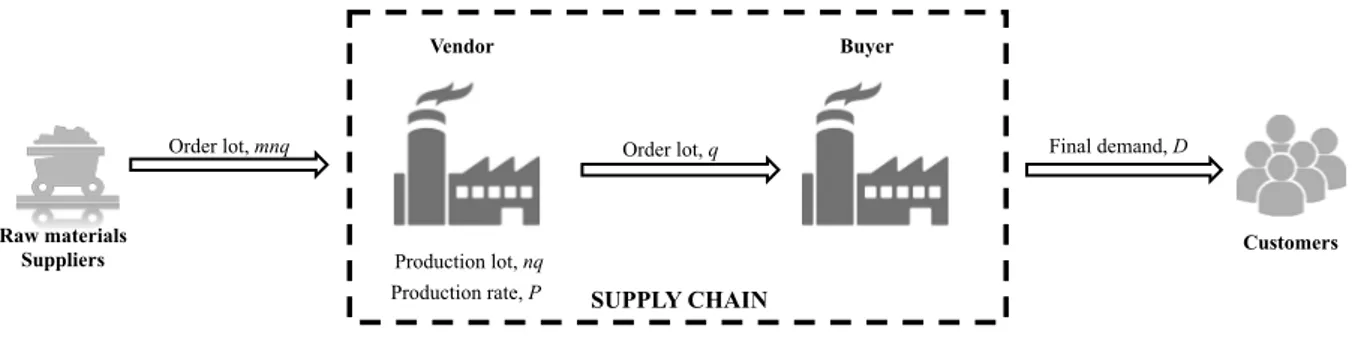
We consider a vendor that produces a single item at a production rate 𝑃 and sells it to the buyer to meet the demand of the end customer, 𝐷 (see Fig. 1). In particular, the vendor needs to purchase 𝛼 units of a high-value storable raw material (e.g., stainless steel), listed in the derivatives market, for producing one unit of finished product. The vendor purchases a quantity of raw material equal to the exact need for 𝑚 production cycles, and it delivers finished products to the buyer in 𝑛 batches of constant size, equal to 𝑞 (with 𝑚, 𝑛 ≥ 1 and integers). According to this description, finished products are manufactured in lots of size 𝑄 = 𝑛𝑞. For the delivery of each batch, it is not necessary to wait for the completion of the production lot 𝑄. Since the considered model refers to a single vendor and a single buyer, and the quantity transported is always equal to 𝑞, it was decided to include the fixed transport costs within the buyer ordering costs. The holding costs are given by two contributions: i.e., a physical and a financial component. The former represents those costs deriving from the handling and storage of the goods; the latter, instead, represents a hidden cost, deriving from capital immobilization. In particular, the financial holding cost is evaluated as a function of the value of the stocked items, which varies along the supply chain. The peculiarities of the models proposed in this work lie in considering a volatile price of the raw material and in the opportunity that the vendor has to protect itself from the commodity risk, without transferring it to the buyer. For instance, if the vendor begins to produce and it may set the selling price of the finished product only when the order is received, it is the customer who takes the commodity risk. In this case, in fact, the price of the finished good is fixed on the basis of the actual value of the raw material, i.e., the price that the vendor pays to buy the goods in order to start producing. In the models dealt with, it is instead considered that the vendor purchases the raw material at time 𝑡 and it resells the products to the buyer at a later time 𝑡 + 𝑘 and at a price that is a function of the cost of the raw material in 𝑡 + 𝑘. In doing so, the vendor assumes high risks. Nevertheless, it has the opportunity to implement strategies for preventing the erosion of the profits or, in the worst case, for avoiding a loss. In this study, we assumed that the vendor can select among two different strategies in order to protect itself from the volatility of raw materials prices: i.e., (a) to give to the banks a part of the stock as collateral, obtaining a discount on the interest rates applied, thus succeeding in reducing the cost of capital, and (b) to use futures contracts to hedge the raw material stocks.

In this simplified formulation of the problem, the number of production cycles covered by each order of raw materials does not represent a decision variable, since its optimal value would always correspond to one. This is due to the fact that the production cycle is assumed to be repeated infinitely at the same conditions. Hence, increasing the m value would only increase the raw material holding cost. While, in order to contrast significantly large order costs, the vendor would increase the production lot size (𝑛𝑞), which introduces larger benefits.

Other assumptions, relevant to the development of the models, are listed hereafter:

- A single-vendor single-buyer supply chain is considered under a centralized decision-making process. - The time horizon is infinite.

- The final demand rate 𝐷 is deterministic and constant over time.

- The production rate P is deterministic, constant and greater than the demand rate (𝑃 > 𝐷). - No stockout is allowed at the costumer ends.

(7)

- The unit cost of the raw material is modelled by a probability distribution, the density function of which is 𝑓(𝑥).

Fig. 1 Schematic representation of the supply chain

3.3. Development of the models

In this section, a JELS model with two alternative inventory management policies (i.e., a backward policy, based on the classical model proposed by Hill, and forward coordination, based on a consignment stock agreement) will be implemented for three different scenarios. In detail, these scenarios are: the basic one without any form of financing practice (Scenario 0), the scenario with the implementation of the warehouse financing practice (Scenario 1), and the scenario which considers the stock hedging by futures contracts (Scenario 2).

3.3.1. Backward and forward JELS models (Scenario 0)

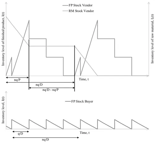
The first scenario represents the classical inventory model, without any type of financial policy, and it will be considered as the reference case against which the economic performances of the two alternative scenarios will be compared. Firstly, we consider a backward coordination policy among the vendor and the buyer, based on the model proposed by Hill (1999), in which the finished products are stored in the vendor's warehouses until the buyer order arrives. The related inventory levels of raw materials and finished products in the warehouses of the vendor and the buyer are shown in Fig. 2.

The quantity of raw materials ordered by the vendor covers 𝑚 production cycles. Hence, the first production cycle is characterized by a larger amount of stock, which decreases as the production cycles run. For this reason, the ordering and holding costs per cycle, related to the purchase of raw materials, should be multiplied for an annual number of cycles (𝐷 𝑚𝑛𝑞⁄ ), which may differ from the number of production cycles (𝐷 𝑛𝑞⁄ ).

Vendor Buyer Raw materials Suppliers Order lot, q Production lot, nq Final demand, D

Production rate, P _{SUPPLY CHAIN}

Customers

(8)

Fig. 2 Inventory levels of the warehouses under the backward policy: stocks of raw materials (‘RM Stock Vendor’) and

finished products (‘FP Stock Vendor’) at the vendor warehouse, and stock of finished product at the buyer warehouse (‘FP Stock Buyer’).

The total cost function is given by the setup cost, the ordering cost of the vendor and the buyer, the holding costs related to the stock of raw materials and finished product at the vendor’s and buyer’s warehouses, and the profits or losses due to the variation in the raw material price. In particular, the vendor, and consequently the overall supply chain, will incur in potential revenues (costs) if the price rises (decreases) with respect to 𝑟.

𝑇𝐶'()**(𝑞, 𝑛, 𝑃) = C 𝑆 𝑛+ 𝐴# 𝑛 𝑚+ 𝐴"D 𝐷 𝑞+ E α 𝑛𝑞 2 𝐷 𝑃+ H(𝑚 − 𝑗) α 𝑛𝑞 𝑚 + ,-. K ℎ!+ 𝑞 2LC1 − 𝐷 𝑃D 𝑛 + 2𝐷 𝑃 − 1M ℎ# +𝑞 2ℎ"+ NO(𝑟 − 𝑥)𝑓(𝑥)𝑑𝑥 − ! ' O(𝑥 − 𝑟)𝑓(𝑥)𝑑𝑥 / ! Q 𝐷! (1)

where ℎ!= ℎ!,&+ ℎ!,$, ℎ!,&= 𝑟(𝜌'+ 𝜌), ℎ#= ℎ#,&+ ℎ#,$, ℎ#,&= R𝛼𝑟 + 𝑐$S(𝜌'+ 𝜌), ℎ"= ℎ",&+ ℎ",$, and ℎ",&= R𝛼𝑟 + 𝑐$S(1 + 𝛿)(𝜌'+ 𝜌).

Then, we consider an inventory management policy based on a forward coordination among the two players, as defined by a consignment stock (CS) agreement (Braglia and Zavanella 2003). Under this policy, the vendor stocks the finished products directly at the buyer warehouse. Despite this, however, the ownership of the goods remains of the vendor, until the buyer picks them up for their use or resell. The related inventory level of raw materials and finished products in the warehouses of the vendor and the buyer are shown in Fig. 3. The main advantage obtained by the CS approach lies in the

0 00 Inve nt or y l eve l of r aw m at er ia l, Ir (t) Inve nt or y l eve l of f ini she d pr oduc t, I (t ) Time, t FP Stock Vendor RM Stock Vendor 0 0 Inve nt or y l eve l, I (t ) Time, t FP Stock Buyer nq/P q/D nq/D nq/D nq/D - nq/P

(9)

reduction of the overall holding costs if ℎ#,&< ℎ",&, which usually occurs due to an increase of the value of the goods along the supply chain, or to different financial conditions of the actors (e.g., the vendor is a multinational company with lower interest rates while the buyer is a SME), or if ℎ",$ < ℎ#,$ (e.g., the vendor has multiple demands to satisfy and a limited warehouse’s capacity).

Fig. 3 Inventory levels of the warehouses under the forward policy: stocks of raw materials (‘RM Stock Vendor’) and

finished products (‘FP Stock Vendor’) at the vendor warehouse, and stock of finished product at the buyer warehouse (‘FP Stock Buyer’).

Equation (2) defines the total cost for the supply chain under a consignment stock agreement in Scenario 0.

𝑇𝐶'01(𝑞, 𝑛, 𝑃) = C 𝑆 𝑛+ 𝐴# 𝑛 𝑚+ 𝐴"D 𝐷 𝑞+ Eα 𝑛𝑞 2 𝐷 𝑃+ H(𝑚 − 𝑗) α 𝑛𝑞 𝑚 + ,-. K ℎ!+ 𝑞𝐷 2𝑃ℎ#+ 𝑞 2LC1 − 𝐷 𝑃D 𝑛 + 𝐷 𝑃M ℎ01 + NO(𝑟 − 𝑥)𝑓(𝑥)𝑑𝑥 − ! ' O(𝑥 − 𝑟)𝑓(𝑥)𝑑𝑥 / ! Q 𝐷! (2) where ℎ'01= ℎ#,&+ ℎ",$.

3.3.2. Backward and forward JELS models with warehouse financing (Scenario 1)

The costs and benefits introduced by implementing the warehouse financing practice derive from two variations which, according to their nature, can bring gains or losses to the company: i.e., variations in the capital and in the raw materials costs. The first variation is closely linked to the use of the warehouse financing, while the second derives from the fact

0 00 Inve nt or y l eve l of r aw m at er ia l, I r (t) Inve nt or y l eve l of f ini she d pr oduc t, I (t ) Time, t FP Stock Vendor RM Stock Vendor 00 Inve nt or y l eve l, I (t ) Time, t FP Stock Buyer nq/P q/D nq/D nq/D nq/D - nq/P

(10)

that the company does not hedge its stock from the commodity risk, as in Scenario 0. The financial institution decides the discount to be applied to the interest rate (and, consequently, to the capital cost) on a case-by-case basis, especially taking into account the state of liquidity, the type and the value of the asset. However, it is clear that the larger the level of inventory used as a guarantee, the larger the discount that the bank will be able to apply. This is due to the fact that the larger the value of the goods left as collateral, the lower the risk of insolvency. Generally, this strategy can provide interest-free financing, except for a small service fee (𝜌') to obtain the banker’s acceptance (Lin et alii 2018). The capital cost for the scenario with warehouse financing can be modelled as follows:

𝜌2_{= 𝜌} '+

𝜌

𝛽 𝜃 𝜔 𝐼! (3)

where, 𝛽 represents a coefficient defining the elasticity of the capital cost with respect to the stock level, 𝜃 the share of the inventory level used as a guarantee, 𝜔 the liquidity of the goods defining how easily they can be converted into cash, and 𝐼! the average level of inventory, which is equal to α 34₅ 6₇+ ∑+,-.(𝑚 − 𝑗) α 34₊.

The benefits related to the implementation of the warehouse financing practice are taken into account in the evaluation of the holding costs. The total cost formulation becomes:

𝑇𝐶.()**(𝑞, 𝑛, 𝑃) = C 𝑆 𝑛+ 𝐴# 𝑛 𝑚+ 𝐴"D 𝐷 𝑞+ Eα 𝑛𝑞 2 𝐷 𝑃+ H(𝑚 − 𝑗) α 𝑛𝑞 𝑚 + ,-. K ℎ!2 + 𝑞 2LC1 − 𝐷 𝑃D 𝑛 + 2𝐷 𝑃 − 1M ℎ#2 +𝑞 2ℎ"+ NO(𝑟 − 𝑥)𝑓(𝑥)𝑑𝑥 − ! ' O(𝑥 − 𝑟)𝑓(𝑥)𝑑𝑥 / ! Q 𝐷! (4)

with ℎ)2= ℎ),&2 + ℎ),$ (𝑖 = 𝑟, 𝑣), ℎ2!,& = 𝑟𝜌2, and ℎ#,&2 = R𝛼 𝑟 + 𝑐$S𝜌2.

𝑇𝐶.01(𝑞, 𝑛, 𝑃) = C 𝑆 𝑛+ 𝐴# 𝑛 𝑚+ 𝐴"D 𝐷 𝑞+ Eα 𝑛𝑞 2 𝐷 𝑃+ H(𝑚 − 𝑗) α 𝑛𝑞 𝑚 + ,-. K ℎ!2 + 𝑞𝐷 2𝑃ℎ#2 + 𝑞 2LC1 − 𝐷 𝑃D 𝑛 + 𝐷 𝑃M ℎ012 + NO(𝑟 − 𝑥)𝑓(𝑥)𝑑𝑥 − ! ' O(𝑥 − 𝑟)𝑓(𝑥)𝑑𝑥 / ! Q 𝐷! (5) with ℎ012 = ℎ#,&2 + ℎ",$.

3.3.3. Backward and forward JELS models with futures (Scenario 2)

In this model, the vendor decides to protect himself from the commodity risk by hedging its raw material stock with futures contracts, in order to avoid losses resulting from the inventory depreciation. The following additional assumptions are required:

(11)

- the hedge ratio is equal to 1, i.e. the commodity price is perfectly correlated to the value of the futures contract, so as to guarantee that the profits (losses) deriving from the contract are perfectly compensated by losses (profits) due to the changes in the price of raw materials;

- all the stocks in the warehouse are covered using futures.

The relevant costs for hedging the warehouse by futures contracts, considering the assumptions presented so far, are given by fixed costs, for the assessment of the contract, and figurative costs, related to the variability of the raw material price. Specifically, the fixed costs are due to the advanced payment of a share of the contract value (e), used to guarantee the functioning of the Mark to Market accounting method, typical of futures contracts. Since this share will be returned, the cost is related to the immobilization of capital, which could be invested in a different way. Moreover, if, as assumed, the vendor enters the futures market in a short position, and ensures the stocks at the current price 𝑟, it is clear that whether the price will fall below 𝑟 at the end of the contract, the vendor will obtain a positive result (a figurative profit) from the hedge, whereas, whether the price of the raw material should rise, the vendor would get a loss (a figurative cost). Whit respect to the scenario without any technique of stock hedging (scenario 0), the costs and benefits related to the adoption of futures contracts should be added in the total cost formulation.

𝑇𝐶5()**(𝑞, 𝑛, 𝑃) = C 𝑆 𝑛+ 𝐴# 𝑛 𝑚+ 𝐴"D 𝐷 𝑞+ Eα 𝑛𝑞 2 𝐷 𝑃+ H(𝑚 − 𝑗) α 𝑛𝑞 𝑚 + ,-. K ℎ!+ 𝑞 2LC1 − 𝐷 𝑃D 𝑛 + 2𝐷 𝑃 − 1M ℎ# +𝑞 2ℎ"+ e Eα 𝑛𝑞 2 𝐷 𝑃+ H(𝑚 − 𝑗) α 𝑛𝑞 𝑚 + ,-. K 𝑟(𝜌'+ 𝜌) + N− O(𝑟 − 𝑥)𝑓(𝑥)𝑑𝑥 + ! ' O(𝑥 − 𝑟)𝑓(𝑥)𝑑𝑥 / ! Q 𝐷! (6)

𝑇𝐶501(𝑞, 𝑛, 𝑃) = C 𝑆 𝑛+ 𝐴# 𝑛 𝑚+ 𝐴"D 𝐷 𝑞+ Eα 𝑛𝑞 2 𝐷 𝑃+ H(𝑚 − 𝑗) α 𝑛𝑞 𝑚 + ,-. K ℎ!+ 𝑞𝐷 2𝑃ℎ#+ 𝑞 2LC1 − 𝐷 𝑃D 𝑛 + 𝐷 𝑃M ℎ01 + e Eα 𝑛𝑞 2 𝐷 𝑃+ H(𝑚 − 𝑗) α 𝑛𝑞 𝑚 + ,-. K 𝑟(𝜌'+ 𝜌) + N− O(𝑟 − 𝑥)𝑓(𝑥)𝑑𝑥 + ! ' O(𝑥 − 𝑟)𝑓(𝑥)𝑑𝑥 / ! Q 𝐷! (7)

3.4. Solution procedure for the models

The procedure for evaluating the existence of a global optimum is the same for each scenario. At first, the Hessian matrix is obtained, as defined in equation (8), and analyzed in order to determine whether the total cost is convex, i.e. it presents a minimum, in the decision variables (𝑑𝑒𝑡(𝐻) > 0).

(12)

𝐻 = ⎝ ⎜ ⎜ ⎜ ⎜ ⎛ 𝜕𝑇𝐶)85(𝑞, 𝑛, 𝑃) 𝜕𝑞5 𝜕𝑇𝐶)85(𝑞, 𝑛, 𝑃) 𝜕𝑛𝜕𝑞 𝜕𝑇𝐶)85(𝑞, 𝑛, 𝑃) 𝜕𝑃𝜕𝑞 𝜕𝑇𝐶)85(𝑞, 𝑛, 𝑃) 𝜕𝑞𝜕𝑛 𝜕𝑇𝐶)85(𝑞, 𝑛, 𝑃) 𝜕𝑛5 𝜕𝑇𝐶)85(𝑞, 𝑛, 𝑃) 𝜕𝑃𝜕𝑛 𝜕𝑇𝐶)85(𝑞, 𝑛, 𝑃) 𝜕𝑞𝜕𝑃 𝜕𝑇𝐶)85(𝑞, 𝑛, 𝑃) 𝜕𝑛𝜕𝑃 𝜕𝑇𝐶)85(𝑞, 𝑛, 𝑃) 𝜕𝑃5 _⎠ ⎟ ⎟ ⎟ ⎟ ⎞ (8)

where 𝑖 represents the scenario (𝑖 = 0, 1, 2) and 𝑘 the coordination policy (𝑘 = 𝐻𝑖𝑙𝑙, 𝐶𝑆) considered.

Once shown that the total cost function presents a global minimum, the first derivative in 𝑞 is set equal to zero in order to obtain the following optimal lot sizes, respectively for Scenario 0, 1, and 2 under the two coordination policies.

𝑞'()**∗= c d𝑆_{𝑛 +} 𝐴# 𝑛 𝑚 + 𝐴"e 𝐷 f α 𝑛2𝐷𝑃 + (𝑚 − 1) α 𝑛2g ℎ!+ 12fd1 −𝐷_{𝑃e 𝑛 +}2𝐷_{𝑃 − 1g ℎ}#+ 12ℎ" (9) 𝑞'01∗= c d_{𝑛 +}𝑆 𝐴# 𝑛 𝑚 + 𝐴"e 𝐷 f α 𝑛2𝐷𝑃 + (𝑚 − 1) α 𝑛2g ℎ!+ 𝐷_{2𝑃 ℎ}#+ 12 fd1 −𝐷_{𝑃e 𝑛 +}𝐷_{𝑃g ℎ}01 (10) 𝑞.()**∗= ⎷ ⃓ ⃓ ⃓ ⃓ ⃓ ⃓ ⃓ ⃓ ⃓ j d𝑆_{𝑛 +} 𝐴# 𝑛 𝑚 + 𝐴"e 𝐷 f α 𝑛2𝐷𝑃 + (𝑚 − 1) α 𝑛2g R𝑟𝜌'+ ℎ!,$S + 1 2 fd1 −𝐷𝑃e 𝑛 +2𝐷𝑃 − 1g kR𝛼 𝑟 + 𝑐$S𝜌'+ ℎ#,$l + 12ℎ" (11) 𝑞.01∗= ⎷ ⃓ ⃓ ⃓ ⃓ ⃓ ⃓ ⃓ ⃓ ⃓ j d_{𝑛 +}𝑆 𝐴# 𝑛 𝑚 + 𝐴"e 𝐷 f α 𝑛2𝐷𝑃 + (𝑚 − 1) α 𝑛2g R𝑟𝜌'+ ℎ!,$S + 𝐷_{2𝑃 dR𝛼 𝑟 + 𝑐}$S𝜌'+ ℎ#,$e + 1 2 fd1 −𝐷𝑃e 𝑛 +𝐷𝑃g kR𝛼 𝑟 + 𝑐$S𝜌'+ ℎ",$l (12) 𝑞5()**∗= c d𝑆_{𝑛 +} 𝐴# 𝑛 𝑚 + 𝐴"e 𝐷 f α 𝑛2𝐷𝑃 + (𝑚 − 1) α 𝑛2g Rℎ!+ 𝜀𝑟(𝜌'+ 𝜌)S + 12fd1 −𝐷_{𝑃e 𝑛 +}2𝐷_{𝑃 − 1g ℎ}#+ 12ℎ" (13) 𝑞501∗= c d_{𝑛 +}𝑆 𝐴# 𝑛 𝑚 + 𝐴"e 𝐷 f α 𝑛2𝐷𝑃 + (𝑚 − 1) α 𝑛2g Rℎ!+ 𝜀𝑟(𝜌'+ 𝜌)S + 𝐷_{2𝑃 ℎ}#+ 12 fd1 −𝐷_{𝑃e 𝑛 +}𝐷_{𝑃g ℎ}01 (14)

Then, introducing the optimal lot size obtained, 𝑞∗_{, into the total cost function 𝑇𝐶}

)8(𝑞∗, 𝑛, 𝑃), a closed expression of the optimal number of shipments between the vendor and the buyer 𝑛∗_{can be obtained. The formulations, respectively for}

(13)

Scenario 0, and 2 under the two coordination policies, are defined below. While in Scenario 1, it is difficult to obtain a closed-form for the optimal number of shipments, hence, it can be numerically determined (Chang et alii 2005).

𝑛'()**∗= c d𝑆 +𝐴# 𝑚e fd2𝐷𝑃 − 1e ℎ#+ ℎ"g 𝐴"nf α 𝐷_{𝑃 + (𝑚 − 1) αg ℎ}!+ d1 − 𝐷_{𝑃e ℎ}#o (15) 𝑛'01∗= c d𝑆 +𝐴# 𝑚e𝐷𝑃 (ℎ#+ ℎ01) 𝐴"nf α 𝐷_{𝑃 + (𝑚 − 1) αg ℎ}!+ d1 − 𝐷_{𝑃e ℎ}01o (16) 𝑛5()**∗= c d𝑆 +𝐴# 𝑚e fd2𝐷𝑃 − 1e ℎ#+ ℎ"g 𝐴"nf α 𝐷_{𝑃 + (𝑚 − 1) αg Rℎ}!+ 𝜀𝑟(𝜌'+ 𝜌)S + d1 − 𝐷_{𝑃e ℎ}#o (17) 𝑛501∗= c d𝑆 +𝐴# 𝑚e𝐷𝑃 (ℎ#+ ℎ01) 𝐴"nf α 𝐷_{𝑃 + (𝑚 − 1) αg Rℎ}!+ 𝜀𝑟(𝜌'+ 𝜌)S + d1 − 𝐷_{𝑃e ℎ}01o (18)

Since 𝑛 represents the number of shipments between the vendor and the buyer, its value should be an integer one. Hence, 𝑇𝐶)8(𝑞∗, 𝑛, 𝑃) is evaluated by rounding down and up 𝑛∗. The number of shipments leading to the lowest average cost is kept as the optimal value. Due to the complexity of the function obtained by substituting 𝑛∗_{into the total cost function,} 𝑇𝐶)8(𝑞∗, 𝑛∗, 𝑃), it is difficult to reach a closed-form also for the third decision variable, 𝑃. However, the optimal value for the production rate, at which the process runs (𝑃∗_{), can be numerically obtained (Chang et alii 2005), too.}

4. Numerical analysis

4.1. Data

This section presents a numerical study to illustrate the behaviour of the models with different financing solutions and coordination policies, as developed above. We firstly introduce a set of parameters to define a base case study, and then propose some sensitivity analyses by varying relevant parameters in order to take more general insights from the study. Let us consider a vendor-buyer system with the following parameters: 𝛼 = 0.3 kg/unit, 𝐴" = 100 €/order, 𝐴# = 75 €/order, 𝛽 = 50%, 𝑐$ = 5 €/unit, 𝛿 = 25%, 𝐷 = 1000 unit/year, ℎ",$ = 2.5 €/year unit, ℎ#,$ = 7.5 €/year unit, ℎ!,$ = 5 €/year kg, 𝜌' = 5%, 𝜌 = 15%, 𝑟 = 3 €/kg, 𝑆 = 400 €/setup. It is assumed also that the production rate can vary in the range [𝑃+)3= 1000; 𝑃+:; = 3000] unit/year. The unit cost of the raw material is modelled as a normal distribution, i.e. 𝑟 = 𝑁(𝑟̅, 𝜎), with 𝑟̅ = 2 €/unit representing the mean value, while 𝜎 = 1 €/unit the standard deviation. Hence, 𝑓(𝑥) =

. <5=>!𝑒

?(#$%&)!_!(! _{. The company uses, as a guarantee, all the stock in the inventory (i.e., 𝜃 = 100%) and the liquidity of the}

product is set to 20%. The share of the futures value, that should be paid in advance for the establishment of the contract, e, is assumed to be equal to 0.3. Next, we examine the three scenarios mentioned under the two coordination policies, so as to gain insights into the behavior of the models.

(14)

4.2. Results and discussion

Table 1 shows the results of the three scenarios under the backward and forward policies. In all the scenarios, the consignment stock performs better than the traditional agreement based on Hill’s model, since the buyer has a lower physical holding cost than the vendor. Specifically, the CS policy allows the total cost to be reduced by 7.88%, 10.71%, and 10.07% for Scenario 0, 1, and 2, respectively. It emerges also how the financial collaboration, among the two actors, significantly enhances the benefits introduced by the implementation of the CS policy with respect to the traditional one. For the specific case study, the use of futures to hedge the stock leads to a reduction of -17.04% and -19.02% (for the traditional agreement and the CS policy, respectively) with respect to the reference scenario. On the other side, the warehouse financing introduces lower savings, specifically -3.16% and -6.14%. Furthermore, the optimal results show that the scenarios under the traditional agreement determine a lower-speed production process, and production lot sizes larger than those determined under the CS policy. The motivation is that in the backward coordination policy the vendor keeps the stocks at its own warehouse, while in the forward he pushes more rapidly the stocks to the buyer’s warehouse. In the warehouse financing scenarios, the vendor produces larger lots in both the coordination policies, since the larger the inventory level the higher the discount on the capital cost. The convenience of one financial practice, over the other, is strictly dependent on the parameters used in the case study. In the next subsection, some sensitivity analyses are performed to obtain more general managerial insights.

Table 1. Optimal results for the three scenarios under the traditional agreement and the CS policies.

Scenario 0 Scenario 1 Scenario 2

Hill CS Hill CS Hill CS

𝑃∗ _unit/year ₁₀₀₀ ₃₀₀₀ ₁₀₀₀ ₃₀₀₀ ₁₀₀₀ ₃₀₀₀ 𝑛∗ _shipments ₆ ₃ ₆ ₃ ₆ ₃ 𝑞∗ _unit _125.54 _198.14 _130.50 _220.10 _124.66 _197.74 𝑄∗ _unit _753.26 _594.43 _783.02 _660.31 _747.95 _593.21 𝑇𝐶)8(𝑞∗, 𝑛∗, 𝑃∗) €/year 3,131.22 2,884.53 3,032.18 2,707.54 2,597.53 2,335.92 4.3. Sensitivity analyses

In the sensitivity analyses, the scenario without any financing practices under the backward policy is used as the reference case. Then, we investigate the variations introduced in the total cost of the supply chain, i.e. ∆𝑇𝐶)8 =

@0₎*?@0₊

,)--@0₊,)-- . The first

analysis performed considers a variation in the number of raw material shipments, i.e. the number of production cycles covered by a single purchasing order. Higher values of 𝑚 generate larger inventory levels, and consequently higher holding costs. However, in some cases (e.g., when the raw material presents seasonality), the vendor purchases significant amounts of raw materials in order to take advantage of favourable prices. Fig. 4 shows how, for higher 𝑚 values, the benefits introduced by the forward policy and the financing practices are reduced. Specifically, a higher value of 𝑚 reduces the benefits of the consignment stock over the traditional backward policy, if none of the practices described is implemented, and it also reduces the gap between the two financial practices when the traditional backward policy is considered. The scenario with the use of futures and the consignment stock policy represents an exception, since it leads to a larger reduction of the total cost for higher 𝑚 values. It can also be observed that, due to the larger inventory levels, the use of the warehouse financing practices gains relevance. In particular, the scenario with warehouse financing and the forward policy becomes more attractive than the scenario with the use of futures with a backward policy. However, the

(15)

discount achievable through the implementation of the warehouse financing practice presents an upper limit (i.e., the capital cost can decrease from a maximum to the lower limit 𝜌'). Hence, the increase of the raw material inventory level, due to the increase of 𝑚,generates decreasing benefits, and the gap with the scenario without any form of financing practice will stabilize.

Fig. 4 Sensitivity analyses on the variation of supply chain total cost for the different scenarios with respect to the base

case with no financial practices under the traditional agreement, by changing the number of shipments of the raw material (𝑚).

Another interesting parameter is the coefficient that defines how many raw materials are required to produce a unit of finished product. Higher values of 𝛼 leads to larger the demand for raw materials. As Fig. 5 highlights, a larger demand of raw materials increases the benefits introduced by the use of futures contracts for stock hedging, while the scenarios with the warehouse financing practice present an optimal value of 𝛼 that maximizes the reduction in total cost. This is due to the fact that larger inventory levels correspond to higher 𝛼 values, which introduce lower marginal reduction in the capital cost (since 𝜌2_{approaches 𝜌}

'). Hence, for 𝛼 > 0.4, the increase in holding costs is higher than the savings for additional reduction of 𝜌2_{. At the same time, the larger inventory level of raw material introduces a higher commodity} risk, and the use of future contracts allows to protect the company, providing larger benefits in terms of costs.

case with no financial practices under the traditional agreement, by changing the conversion factor of the raw materials to finished products (𝛼). -50% -40% -30% -20% -10% 0% 1 3 5 7 9 DTC m

D TC0,CS_0,Hill D TC1,Hill_0,Hill D TC1,CS_0,Hill

D TC2,Hill_0,Hill D TC2,CS_0,Hill -50% -40% -30% -20% -10% 0% 0,1 0,3 0,5 0,7 0,9 DTC a

(16)

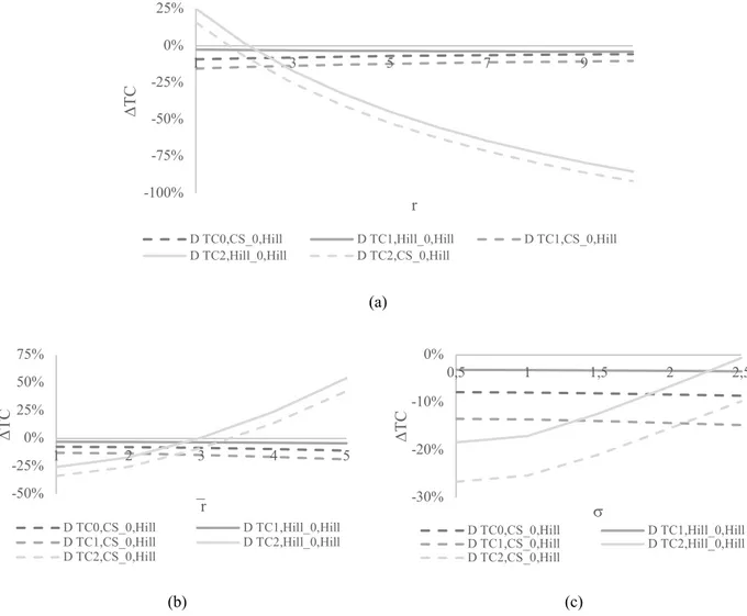
The last analyses concern the price of the raw material. In Fig. 6a, it is shown the variation in the total cost determined by changing the actual cost of the raw material that the vendor should pay for each unit. Fig. 6b shows the results of changes in the average value of the raw material cost. The higher the actual cost, or the lower the average cost, the higher the commodity risk and, hence, the convenience to hedge the stocks with future contracts. This particular practice introduces benefits only if 𝑟 > 𝑟̅, since, otherwise, the vendor must pay the raw material at a higher cost than its final value. At the opposite, the warehouse financing practice introduces higher savings for lower actual unit costs or higher average values, which means a lower commodity risk. Finally, Fig. 6c shows how, for larger variability in the raw material prices (i.e. higher standard deviations), the warehouse financing practice performs better than the use of futures, and hence it represents a more stable practice.

(a)

(b) (c)

case with no financial practices under the traditional agreement, by changing: (a) the cost for a unit of raw material purchased by the vendor, 𝑟, (b) the average value , 𝑟̅, and (c) the standard deviation, 𝜎, of the unit cost of raw material.

5. Conclusions

This paper investigated a single-vendor single-buyer supply chain in which the vendor can adopt two specific financial techniques (i.e., warehouse financing practice and the use of futures contracts) as means for hedging stocks in order to mitigate the commodity risk related to the high volatility of prices. The traditional formulation of the holding cost is also

-100% -75% -50% -25% 0% 25% 1 3 5 7 9 DTC r

D TC2,Hill_0,Hill D TC2,CS_0,Hill -50% -25% 0% 25% 50% 75% 1 2 3 4 5 D TC ̅r D TC0,CS_0,Hill D TC1,Hill_0,Hill D TC1,CS_0,Hill D TC2,Hill_0,Hill D TC2,CS_0,Hill -30% -20% -10% 0% 0,5 1 1,5 2 2,5 DTC s D TC0,CS_0,Hill D TC1,Hill_0,Hill D TC1,CS_0,Hill D TC2,Hill_0,Hill D TC2,CS_0,Hill

(17)

affected by the use of the financial techniques. Specifically, when using the warehouse financing, the financial institution decides a discount to be applied to the interest rate, taking into account the state of liquidity of the company, the type and the value of the asset, which finally affects the financial component of the holding cost. The larger the level of inventory used as a guarantee, the larger the discount that the bank will be able to apply. The two financial practices are included in the traditional joint economic lot size model, under a backward and a forward coordination policy. This study is particularly relevant for companies that have limited market power, since they may hardly transfer the commodity risk to the end customers, e.g. by increasing the wholesale price. An illustrative numerical study was presented to show the behaviour of the developed models. The results highlight that both the financing practices allow the reduction of the total cost of the supply chain. They also show that the scenarios with a backward inventory stocking policy (i.e., Hill approach) present a lower optimal production rate and a larger production lot size, than the scenarios with a forward policy (i.e., based on a Consignment Stock agreement). The motivation is that, under the forward coordination policy, the vendor pushes more rapidly the stocks to the buyer’s warehouse. Furthermore, in the warehouse financing scenario, the vendor produces larger lots under both the coordination policies, since the larger the inventory level, the higher the discount on the capital cost. The results also show that the consignment stock performs better than the traditional backward stocking policy, according to the specific case considered. Furthermore, it emerges that the financial collaboration, among the two actors, highly enhances the benefits introduced by the implementation of the forward policy based on the consignment stock agreement. The convenience of one financial practice over the other is strictly dependent on the parameters used in the case study. Hence, some sensitivity analyses were performed to obtain more general managerial insights. For instance, a larger demand of raw materials increases the benefits introduced by the use of futures contracts for stock hedging, while the scenarios with the warehouse financing practice present an optimal value in the conversion factor of the raw materials into finished products that maximizes the reduction of the overall cost. This is due to the diminishing marginal reduction in the capital cost, when the discounted capital cost approaches the minimum value it can assume.

Companies, generally, should manage different types of products facing, at the same time, several constraints. For example, a company could manage orders for thousands of different products under constraints, such as space, which limit the production (Wang et alii 2012) or may be overcome providing additional warehouse space for each product (Pasandideh et alii 2015), budget (Cárdenas-Barrón et alii 2014), and transportation capacity (Hoque and Goyal 2000; Grunewald et alii 2018). A possible future development of the present work consists in the integration into the models of constraints, such as the ones listed above, which can affect the operational and financial decisions of the firm. Furthermore, other supply chain finance practices, aiming at promoting stability of cash flows, could be investigated, such as the reverse factoring (one of the innovative techniques in supply chain financing, which has received considerable attention from business managers). Furthermore, possible profit-sharing mechanisms, making the centralization of the decisions profitable to both the actors, could represent additional research lines to be encompassed in the models proposed.

References

Aljazzar SM, Jaber MY, Goyal SK (2016) Coordination of a two-level supply chain (manufacturer–retailer) with permissible delay in payments. Int J Syst Sci Oper Logist 3:176–188. doi:

doi.org/10.1080/23302674.2015.1078858

As’ad R, Hariga M, Alkhatib O (2019) Two stage closed loop supply chain models under consignment stock agreement and different procurement strategies. Appl Math Model 65:164–186. doi: 10.1016/j.apm.2018.08.007

Bhunia AK, Shaikh AA, Cárdenas-Barrón LE (2017) A partially integrated production-inventory model with interval valued inventory costs, variable demand and flexible reliability. Appl Soft Comput J 55:491–502. doi:

(18)

10.1016/j.asoc.2017.02.012

Braglia M, Zavanella L (2003) Modelling an industrial strategy for inventory management in supply chains: The “Consignment Stock” case. Int J Prod Res 41:3793–3808. doi: 10.1080/00207540802275863

Cárdenas-Barrón LE, Treviño-Garza G, Widyadana GA, Wee HM (2014) A constrained multi-products EPQ inventory model with discrete delivery order and lot size. Appl Math Comput 230:359–370. doi: 10.1016/j.amc.2013.12.077 Chang SKJ, Chuang JPC, Chen H-J (2005) Short comments on technical note—The EOQ and EPQ models with

shortages derived without derivatives. Int J Prod Econ 97:241–243. doi: 10.1016/j.ijpe.2004.07.002

Gelsomino LM, Mangiaracina R, Perego A, Tumino A (2016) Supply chain finance: a literature review. Int J Phys Distrib Logist Manag 46:348–366. doi: 10.1108/IJPDLM-08-2014-0173

Goel A, Tanrisever F (2017) Financial Hedging and Optimal Procurement Policies under Correlated Price and Demand. Prod Oper Manag 26:1924–1945. doi: 10.1111/poms.12723

Goyal SK (1977) An integrated inventory model for a single supplier-single customer problem. Int J Prod Res 15:107– 111. doi: 10.1080/00207547708943107

Grunewald M, Volling T, Müller C, Spengler TS (2018) Multi-item single-source ordering with detailed consideration of transportation capacities. J Bus Econ 88:971–1007. doi: 10.1007/s11573-018-0894-8

Harris FW (1913) How Many Parts to Make at Once. Factory, Mag Manag 10:135-136,152

Hill RM (1999) The optimal production and shipment policy for the single-vendor single-buyer integrated production-inventory problem. Int J Prod Res 37:2463–2475. doi: 10.1080/002075499190617

Hoque MA, Goyal SK (2000) Optimal policy for a single-vendor single-buyer integrated production-inventory system with capacity constraint of the transport equipment. Int J Prod Econ 65:305–315. doi:

10.1016/S0925-5273(99)00082-1

Kouvelis P, Li R, Ding Q (2013) Managing Storable Commodity Risks : The Role of Inventory and Financial Hedge. Manuf Serv Oper Manag 15:507–521

Kouvelis P, Pang Z, Ding Q (2018) Integrated Commodity Inventory Management and Financial Hedging: A Dynamic Mean-Variance Analysis. Prod Oper Manag 27:1052–1073. doi: 10.1111/poms.12853

Lee W (2005) A joint economic lot size model for raw material ordering, manufacturing setup, and finished goods delivering. Omega 33:163–174. doi: 10.1016/j.omega.2004.03.013

Lin Q, Su X, Peng Y (2018) Supply chain coordination in Confirming Warehouse Financing. Comput Ind Eng 118:104–111. doi: 10.1016/j.cie.2018.02.029

Liu Z, Wang J (2019) Supply chain network equilibrium with strategic financial hedging using futures. Eur J Oper Res 272:962–978. doi: 10.1016/j.ejor.2018.07.029

Marchi B, Ries JMM, Zanoni S, Glock CHH (2016) A joint economic lot size model with financial collaboration and uncertain investment opportunity. Int J Prod Econ 176:170–182. doi: http://dx.doi.org/10.1016/j.ijpe.2016.02.021 Marchi B, Zanoni S, Ferretti I, Zavanella LE (2018) Stimulating investments in energy efficiency through supply chain

integration. Energies 11:. doi: 10.3390/en11040858

Ouyang LY, Ho CH, Su CH (2009) An optimization approach for joint pricing and ordering problem in an integrated inventory system with order-size dependent trade credit. Comput Ind Eng 57:920–930. doi:

10.1016/j.cie.2009.03.011

Pacheco-Velázquez EA, Cárdenas-Barrón LE (2016) An economic production quantity inventory model with backorders considering the raw material costs. Sci Iran 23:736–746

(19)

production quantity model for an imperfect production system under warehouse construction cost. Int J Prod Econ 169:203–214. doi: 10.1016/j.ijpe.2015.08.004

Pfohl H-C, Gomm M (2009) Supply chain finance: optimizing financial flows in supply chains. Logist Res 1:149–161. doi: 10.1007/s12159-009-0020-y

PwC (2009) Navigation: Managing commodity risk through market uncertainty

Sana SS, Chedid JA, Navarro KS (2014) A three layer supply chain model with multiple suppliers, manufacturers and retailers for multiple items. Appl Math Comput 229:139–150. doi: 10.1016/j.amc.2013.12.006

Steinrücke M, Albrecht W (2018) Integrated supply chain network planning and financial planning respecting the imperfection of the capital market. J Bus Econ 88:799–825. doi: 10.1007/s11573-017-0883-3

Taft EW (1918) The most economical production lot. Iron Age 101:1410–1412

Wang SP, Lee W, Chang CY (2012) Modeling the consignment inventory for a deteriorating item while the buyer has warehouse capacity constraint. Int J Prod Econ 138:284–292. doi: 10.1016/j.ijpe.2012.03.029