Decentralized Control of a Swarm of Unmanned Aerial Vehicles

(1)

DECENTRALIZED CONTROL OF A SWARM

OF UNMANNED AERIAL VEHICLES

Tesi di Dottorato

Dottorato di Ricerca in: Automatica, Robotica e Bioingegneria Ciclo XIX (2004)

Supervisore: Prof. Mario Innocenti Studente: Elisabetta Ronchieri

Universit`a degli Studi di Pisa

Dipartimento di Sistemi Elettrici e Automazione

(2)

(3)

Abstract

Several human operators control a single Unmanned Aerial Vehicle. This is not scalable. Recently, the trend is to have a single human operator to handle a group of Unmanned Aerial Vehicles in order to have a system able to work with thousands of Unmanned Aerial Vehicles flying over a country. Swarm Intelligence (the emergent, collective of social insect colonies) provides the guidelines to design such a decentralized system. In particular, social insects are capable of achieving several things, such as building and defending a nest, foraging for food, taking care of the brood, allocating labor, forming bridges.

This thesis presents a framework for decentralized control of a swarm of Un-manned Aerial Vehicles based on the artificial potential functions characterized by attractive and repulsive properties, which are used respectively to achieve the goal and to avoid collisions. Each vehicle of the swarm makes use of lim-ited information from others, and furthermore it is assumed to have a simple dynamic and to be identified as an agent. In this scheme, multiple agents in a swam are able to reach a configuration and to maintain it, while migrating as a group and avoiding collisions among each other. Therefore, the behaviors of the swarm system proposed in this thesis are group migration and configuration, and include collision avoidance.

In particular, this thesis evaluates different potential expressions in order to determine how quickly the swarm converges to a desired direction and velocity, and how robust the swarm is against collisions among the agents. Furthermore, two metrics estimate which potential is the best one in a certain scenario. One quantifies how quickly the swarm converges to the given velocity, and the second evaluates how robust the potential is against collisions. The simulation results show that the proposed scheme can construct a swarm system with the capability of group migration and configuration in the presence of obstacles, by using a

(4)

(5)

Riassunto

Molti operatori controllano un solo Unmanned Aerial Vehicle – Veicolo Aereo Non Equipaggiato – rendendo il sistema di controllo non scalabile. Attualmente, nell’ambito del controllo di questo tipo di veicoli, la tendenza ´e quella di gestire un gruppo di Unmanned Aerial Vehicle tramite un solo operatore in modo da avere un sistema in grado di operare con migliaia di Unmanned Aerial Vehicle che volano sopra una nazione. Swarm Intelligence, basata sui cosiddetti insetti so-ciali, fornisce le linee guida per progettare sistemi decentralizzati. In particolare, gli insetti sociali sono in grado di perseguire diversi obiettivi, dalla costruzione e difesa del nido, alla ricerca del cibo, al prendersi cura del nido, all’assegnazione di squadre di operai, alla costruzione di ponti.

Questa tesi presenta un framework per il controllo decentralizzato di uno sciame di Unmanned Aerial Vehicle basato su funzioni di potentiale artificiale caratterizzate da proprietá attrattive e repulsive, che sono usate rispettivamente per raggiungere l’obiettivo e per evitare le eventuali collisioni. Ciascun veicolo dello sciame utilizza un numero limitato di informazioni degli altri veicoli, ed inoltre é caratterizzato come un agente con dinamica molto semplice. In questo schema, piú agenti di uno sciame sono in grado di raggiungere una configurazione e di mantenerla, mentre migrano come gruppo ed evitano collisioni tra di loro. Pertanto, i comportamenti del sistema a sciame proposto in questa tesi sono la configurazione e la migrazione del gruppo, e includono la elusione di collisioni.

In particolare, questa tesi analizza diverse espressioni di potenziale per deter-minare in quanto tempo lo sciame converge alla direzione e velocitá desiderata, e quanto é capace lo sciame ad evitare le collisioni tra gli agenti. Inoltre, sono state determinate due metriche che forniscono la stima del migliore potenziale in un determinato scenario. Una metrica quantifica quanto velocemente lo sciame converge ad una data velocitá, e la seconda analizza quanto robusto é il

(6)

ziale per evitare le collisioni. Le simulazioni mostrano che la soluzione proposta permette di costruire un sistema a sciame in grado di gestire la migrazione e la configurazione del gruppo in presenza di ostacoli utilizzando un numero limitato di informazioni.

(7)

To Renato, Lia, Massimo, Lucia, and Massimo

(8)

“Data la causa, la natura opera l’effetto nel pi`u breve modo che operar si possa” — Leonardo Da Vinci, (1452-1509)

(9)

Acknowledgments

This thesis would not exist without the help and care of many people. I wish to thank my supervisor, Professor Mario Innocenti, for providing me with valu-able articles, being my source of inspiration at the beginning of my research, communicating his critical judgments on my activity, and supporting me with his expertise, and understanding. Special thanks are due to Charles Loomis of the LAL (Laboratoire de l’Acclrateur Linaire) for reading and commenting each draft version of my papers, produced during the three years of the doctorate course; to Alessandro Quarta and Professor Giovanni Mengali of the DIA (De-partment of Aerospace Engineering) of the University of Pisa for their friendship and support, providing me useful suggestions with fruitful discussions and in-forming me about international conferences and journals; to Professor Andrea Caiti for his support and his invaluable experience and advice; to Roberto Mati for sending me some articles in the latest doctorate year, due to the impossibility to download scientific papers from Bologna where I live.

In addition, I am grateful to the head of Research Division at CNAF, Antonia Ghiselli, for the freedom I was given to pursue my own research activities. A special thank to Tiziana Ferrari who encouraged me to undertake this journey.

Finally, I wish to express my thanks to all my family, in particular to Massimo Concu, my husband, for his patience, constant support and understanding during a long period of hard work and irregular hours over the past years.

(10)

(11)

List of Tables

2.1 Simulation Parameters. . . 24

(14)

(15)

List of Figures

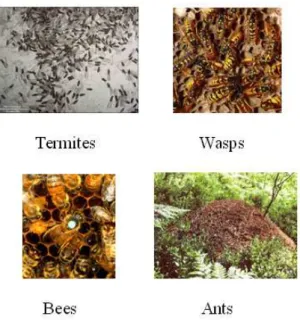
1.1 Swarms of Social Insects (i.e., termites, honey bees, wasps and ants) 3

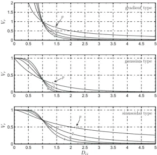
2.1 Behaviour of the selected repulsive potential Vr (e.g., gradient,

gaussian and sinusoidal type) as a function of Dij and p. . . . 15

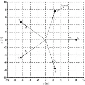
2.2 Initial Scenario Configuration of the agents (at time t = 0). The locations of the five agents are given by: i1(2.4721, 7.6085),

i2(−6.4721, 4.7023), i3(−6.4721, −4.7023), i4(2.4721, −7.6085), i5(8, 0). 19

2.3 Agents Trajectories with sinusoidal potential for Case I. Each tra-jectory is represented by eighteenth time-steps (each of them has been calculated at the same time t), and there is not any overlap-ping. For instance, the third sample for agent i2 corresponds to

the sixteenth sample for agent i1, whilst the seventeenth sample

for agent i4 is among the first two samples for agent i3. . . 21

2.4 Relative Distances among agents in Case I. For each agent it is displayed its distance with all the other agents together with the security distance. According to the resulted trajectory the critical distance is related to the agent i2 with respect to the agent i3. . 22

2.5 Velocity components of the agents in Case I. The final velocity of each agent reaches the desired value v?_{. The vertical and}

hori-zontal scales are the same for each plot. . . 23 2.6 Control Effort ui/mi for five agents in Case I. The vertical and

horizontal scales are the same for each plot. . . 23 2.7 Temporal history of the artificial potential Vi for five agents in

Case I. . . 24 2.8 Trajectories followed by the agents in Case II. . . 25

(16)

2.9 Velocity components of the agents in Case II. The velocity of each agent reaches the desired values v?

1and v?2. The vertical and

horizontal scales are the same for each plot. . . 26 2.10 Control Effort ui/mi for five agents in Case II. The vertical and

horizontal scales are the same for each plot. . . 26 2.11 Initial Scenario Configuration of the agents (at time t = 0). The

initial locations of the two agents are i1(−7, 0) and i1(7, 0), whilst

the locations of the two obstacles are io1(−1, 1) and io2(1, 1). . . 29

(17)

Preface

This thesis is the result of my research made during Ph.D. in Automation, Robotics and Bioengineering at the Department of Electrical Systems and Au-tomation, University of Pisa, under the supervision of Professor Mario Innocenti, from January 2004 and December 2006.

First, this research involves Swarm Intelligence, due to the high number of its successful applications in robotics. It is based on the study of natural collective behaviours in decentralized and self-organized systems. By using this form of artificial intelligence, groups of Unmanned Air Vehicles are simplified in groups of simple agents interacting locally with one another and with their environment. Examples of collective behaviours in nature are ant colonies, bird flocking, animal herding, bacteria molding and fish schooling.

Then, this thesis involves also the new scientific discipline called Biomimicry (from Greek bios – life – and mimesis – imitation), also known as Biomimetrics, due to the recent trends in the solution of engineering problems to design a new class of Unmanned Aerial Vehicles and in the control system design. Biomimicry studies nature’s models, taking ideas from these designs and implementing them in another technology such as engineering or computing. The reason is that nature has come up solutions for different problems such as foraging and survival for food in a hostile environment, swarm behaviour, developing billions of years of trial-and-error. Nature use evolution to solve these problems by using the mechanism of natural selection, involving the adaptation to totally different habits from other years. Furthermore, this new science uses nature to judge the

rightness of human solutions. Also, Biomimicry is based on the concept that

human can learn from natural world, therefore the nature is considered as a mentor.

Some materials of this thesis have been published in the following papers:

(18)

• E. Ronchieri et al., ”The Biomimicry in UAV Control Systems Design”, 15th International Symposium on Measurement and Control in Robotics, ISMCR05, Brussels, Belgium, November 2005.

• E. Ronchieri et al., ”Non Linear Control Applied to a Swarm of Unmanned

Air Vehicles”, 9th International Symposium on Climbing and Walking

Robots and Associated Technologies, 11 – 14 September 2006, Royal Mil-itary Academy, Brussels, Belgium.

• E. Ronchieri, M. Innocenti, ”Decentralized Control of a Swarm of

Un-manned Aerial Vehicles”, accepted to AIAA Guidance, Navigation, and

Control Conference & Exhibit, 20 – 23 August 2007, South Carolina, USA.

Contribution

The purpose of this thesis is to give a coherent understanding of swarm be-haviours through artificial potential and to provide an insect flight model.

Outline

This dissertation is tailored for a wide audience including engineers as well as biologists interested in swarm behaviours applied to Unmanned Aerial Vehicles from a control theory perspective.

Chapter 1 serves as introduction to the thesis and establishes the philosophy of the general methodologies that are used. First, we provide an overview of the social insects in order to describe some of the natural collective behaviours. Then, we explain why the requirements of Unamanned Aerial Vehicles can be satisfy by nature. Next, we overview some ideas from biology applied to Un-manned Aerial Vehicles.

Chapter 2 introduces the artificial potential method. First, we provide the basics of the artificial potential and explain when this method is suitable. Next, we introduce the problem statement and explain our solution with the artificial potential function. Then, case study is described together with the results from the numerical simulations obtained for a single goal. Therefore, our reflections are reported with the definitions of two metrics. In addition, simulations and results are also provided for a sequential of targets in order to show that the swarm is able to change trajectory and maintain its alignment once a target

(19)

is reached. The problem statement is extended to also consider the obstacles. Finally the conclusions are reported.

Finally, Chapter 3 summarizes the results presented in the dissertation and discusses possible extensions, in particular from a theoretical perspective.

(20)

(21)

Chapter 1

Introduction

Evolution has already resolved many of the challenges found in nature providing solutions characterized by having maximal performance and using minimal re-sources. Through evolution, nature has produced effective solutions to complex real-world problems responding to its needs in harmony with the environment. Therefore, it has inspired humans in their desire to improve their life and led to effective algorithms, methods, materials, structures, mechanisms and systems. Biomimicry, also known as Biomimetics, involves copying, imitating and learn-ing from biology. It has been applied to a number of fields from political science to car design to computer science (e.g., cybernetics, swarm intelligence, artificial neurons and artificial neural networks are all derived from biomimetic princi-ples), helping humans understand related phenomena and associated principles in order to engineer novel devices and improve their capability.

Before discussing social insects, it is important to recognize that the majority of biological creatures are made up by a cell-based structure that offers them the ability to grow with fault-tolerance and self-repair. It is also interesting to observe that workable solutions found in nature pass the test of survival in order to reach the next generation. In particular, Lowman [21] observed that the presence of life on Earth dates back to 3.8 billion years ago; Schopf [31] noticed that ancient bacteria, called Archea (Archaebacteria), have existed on the Earth for at least 3.5 billion years. Notice, however, that the evolution of mega-scale terrestrial biology failed with the extinction of creatures such as dinosaurs and mammoths, whilst marine creatures such as whales survived.

(22)

1.1 Social Insects

Insects, part of social category, live in colonies, such as ants, bees, wasps and termites. Each of them is self-organized, and specialized in a set of tasks, ac-cording to its morphology, age, or change. Therefore, these organisms perform various activities simultaneously inside the colony, displaying collective swarm intelligence.

For example, individual termite could not build nests without the collab-oration of the others, whilst ants allocate labor dynamically to different tasks. Honey bees build series of parallel combs, each of them is organized in concentric rings of brood, pollen and honey. In addition, honey bees search food sources according to their quality and the distance from the hive. Some termites build complex nests characterized by a cone-shaped outer walls. A swarm of tropical termites can build complex multilevel mounds that can be five meters tall and weigh ten tons [25]. In particular, these mounds have impressive overall rigidity, are made from a material that is fire resistant, and contain enough rooms and passages to house the brood and all of its food reserves. There are many other examples of the capabilities of social insects [5] and Figure 1.1 collects some swarms of social insects.

Social insect colonies are able to connect individual behaviour with collective performance. Some aspects of the collective activities of social insects are self-organized, and therefore complex collective behaviours can emerge from inter-actions among individuals with simple behaviour [14]. Typical problems solved by a colony include finding food, building or extending a nest, dividing labor among individuals, feeding the brood, and responding to external challenges, for instance. Insects solve these problems in a very flexible and robust way. In fact they are able to adapt themselves when the environment changes (i.e., flex-ibility), and to collaborate each other in achieving the colony task even though some of them fail to perform their tasks. It is important to observe that a social insect colony is a decentralized problem-solving system, comprised of many sim-ple interacting entities. Social insects can be modeled by using self-organization theories.

Individual ants gather together to perform complex social tasks such as aphid farming. These farming ants protect a herd of smaller insects from predators so they can milk them of their honeydew [16]. Also, most ant species form invisible roadways, called ant highways, where columns of ants follow one another

(23)

Figure 1.1: Swarms of Social Insects (i.e., termites, honey bees, wasps and ants)

without the aid of street signs or painted lanes. These complex behaviors are accomplished via pheromones. In this dissertation, pheromone is not taken into consideration. Only the self-organization is analyzed.

1.2 Swarm of Unmanned Aerial Vehicles

Common Unmanned Aerial Vehicle (UAV) requires at least two operators, one to fly the plane and the other to mange the camera mounted on it. More commonly, four people are needed. It is interesting to observe that in some cases the field of view afforded to the pilot is poor, therefore when a vehicle operates in a hostile environment, the pilot loses knowledge of location. If the situation is so critical for one UAV, thousands of people will be necessary to control a swarm of Unmanned Aerial Vehicles (UAVs). This situation can be improved by the future UAVs with more autonomous flight capabilities. However, even with such advanced UAVs, they will still require human supervision to know where to go and to confirm sensitive actions. Therefore, further improvement of UAV

(24)

ground control stations will be necessary as they are inadequate for controlling and monitoring the progress of a swarm of UAVs.

Some UAVs are already capable of taking off, flying a specified path, and landing on their own, reducing the presence of humans. UAVs should be designed in order to leave just one person in the loop of control, be it for a single UAV or an entire swarm of them. In order to achieve that, a system enables to support simple controls that perform tasks without the knowledge of the entire system, but whose combined actions exhibit complex aggregate behavior. In addition, a swarm of UAVs should be kept as simple as possible to minimize costs, to enhance their robustness in the field, and to perform complex tasks as a whole. Nature has provided a template for accomplishing these requirements in social insects. A swarm control algorithm can be created by making analogies among UAVs and social insects. Social insects have a complex aggregate behavior despite being simple creatures.

A swarm of UAVs can be considered as a set of N agents (typically ten or more), which cooperate with each other to achieve some behavior and some goal, moving in a way that appears to be well-choreographed but following simple rules to guide their actions. The swarm achieves its goal via the interactions with all the entities. In Ref. [20] an overview of the intelligent swarm behavior is given as the emergent collective intelligence of groups of simple autonomous agents. It describes some application areas for swarm intelligence such as swarm robots, biological basis and artificial life.

1.3 Related Works

Scientists from multiple disciplines have recently begun to model biological swarms to better understand how social animals (i.e., birds, insects, fish) inter-act, achieve goals, and evolve [30]. Through billions of years of trial-and-error using the mechanism of natural selection, nature has chosen specific solutions to problems such as survival and foraging for food in a hostile environment, involv-ing the adaptation to totally different habits. Many of these solutions involve swarm behavior and can be used as a source of inspiration by analogy, to pro-vide enhanced solutions in the control management of UAVs for civil [22], space missions [1, 26], and military [24] applications.

New technologies permit the development of new vehicles with small (or mi-cro) dimension following methods and systems found in nature, that is using

(25)

Biomimicry. Furthermore, trying to mimic natural emerging systems as swarm-ing [15], reduces the ratio of human operators to control sophisticated UAVs. A typical one is an Unmanned Air Vehicle (UAV) engaged in space missions for scientific investigation, like planetary surface exploration, where the strategies to mission and flight planning can be improved by developing biologically inspired flight control [33, 34]. Another example is the use of UAVs in urban areas to test concentrations of hazardous materials from biological, chemical, or nuclear accidents.

(26)

(27)

Chapter 2

Artificial Potential Fields

Applied to a Swarm

Artificial Potential Fields are mathematical functions, assigned to robots and threats. A force is induced on any robot that is kept in a potential field. Each robot moves to the positions where the potential is the least, as these are the positions where the forces acting on the robot are minimum. Furthermore, this approach works by associating the goal with the location of the lowest potential and making the robots move to this point. The artificial potential theory represents an affordable good way to navigate a swarm in an unknown environment, requiring a low computational cost.

We present a framework for non-linear control of a swarm of agents based on the artificial potential characterised by attractive and repulsive potentials. This artificial potential under certain conditions is conducible to Lyapunov’s potential. In this context, the swarm is able to reach a desired configuration and to maintain it whilst it migrates as a group avoiding inter-agent collisions. Therefore, the behaviors of the swarm system proposed in this study are group migration and configuration, and include collision avoidance. In particular, we define three potential functions specific to the problem under examinations be-longing to three different families present in literature: a gradient, a gaussian and a sinusoid. By examining these potentials we address the guidance problem of a swarm of agents in order to determine how quickly the swarm converges to a desired direction and velocity, and how robust the swarm is against collisions amongst the agents. Furthermore we also provide two metrics that estimate

(28)

which potential is the best one in a certain scenario. The former quantifies how quickly the swarm converges to the given velocity, whilst the latter evaluates how robust the potential is against collisions.

2.1 Role of Artificial Potential

In the past decade, the artificial potential theory have been used for path plan-ning of autonomous mobile robot [4, 11, 12, 19, 28], where a robot is modeled as a particle which moves inside an artificial potential field generated using attrac-tive and repulsive potentials. The former pulls the robot to a goal configuration, whilst the latter pushes robot away from obstacles and collisions. The negative gradient of the generated global potential field is considered an artificial force acting on the robot and dictating its motion. Recently, some of the studies have extended artificial potential methods to the maneuvering of group behaviours in a distributed swarm system composed by a large number of autonomous agents [2].

How to select scaling parameters of the artificial potential functions related to the attractive and repulsive forces in order to avoid the local minima re-mains a challenge. Furthermore the potential field-based methods are oriented heuristically and the lack of analytical design guidelines can be problematic in applications. In Ref. [6] the attractive and repulsive functions are standard defined, therefore the repulsive force is much larger than the attractive one. In this particular case, when the goal is near the obstacle, the robot cannot reach the goal because of the larger repulsive force coming from the obstacle.

Many swarm-like algorithms are based on the concept of artificial potential fields. One characteristic of a system using artificial potential fields is the oc-currence of local potential minima. These algorithms will fail, if the robot gets stuck in one of the local minima. Therefore, systems using such algorithms ei-ther try to change their potential functions in order to avoid local minima, or define a special algorithms. A discussion of social potential fields has been done in [27], providing guidelines to design potential fields in order to achieve certain tasks such as a guarding behaviours for robots and bivouacing. In Ref. [32] the authors have used and analyzed simple artificial potentials to make a group of robots from particular shapes.

A class of attraction and repulsion functions [10, 9] extends the results on swarm aggregations in Ref. [11]. Some theoretical results have been introduced

(29)

on the dynamics of aggregating swarm of robots. In Ref. [8] the potential method is used in order to maneuver group behaviors such as formation, migration and obstacle avoidance in swarm systems. Finally, Refs. [17, 18] presents a satellite path planning algorithm inspired by collective robotics.

2.2 Problem Statement

We assume that the swarm is a set of N agents and, for convenience, we start with a point of mass model in which an individual agent’s motion is based on Newton’s law [23]. Taking this model into account the equations of motion, for the i-th agent (subscript i), are:

˙xi= vi (2.1)

˙vi= ui

mi (2.2)

where xi is the position, vi is the velocity, mi is the mass and ui is the total

applied force (a control law or a set of controls) for the i-th agent. Each agent is characterized at time t = 0 by an initial position xi(0) and a start velocity

vi(0) and a target velocity v∗.

The aim of the swarm is for all agents to reach the same velocity v∗_without

colliding with any of the other agents, that is:

(xi− xj) · (xi− xj) ≥ c2i (2.3)

where xj is the position of the j-th agent closest to the i-th agent with j 6= i,

kxi− xjk is the distance of the i-th agent from the j-th agent, and c2i is a given

constant1_{. The term c}

i represents the smallest permissible distance that has to

be observed for security reason between two agents.

The problem consists of finding a suitable control law ui(t) such that the

i-th agent reaches the velocity v∗ _{and the constraint of Eq. (2.3) is met along}

the agent trajectory.

2.3 Solution with Artificial Potential

This section introduces a proposed control law in order to accomplish the as-signed mission. We suppose to re-configure the swarm of agents in order to allow

1_{The constant c}2

(30)

each agent to reach the desired velocity v∗_{. This also means, at steady-state, to}

execute an alignment of the whole swarm in a given direction coincident with that of the desired velocity. The complexity of the re-alignment problem of the swarm increases when the distance among two or more agents is less than what we consider the security distance ci. In order to avoid catastrophic collisions, the

control law will be able to allow each agent an evasive manoeuvre in a danger scenario.

We observe that this problem is quite difficult to manage because there is a high number of degrees of freedom and the complexity of the system grows quickly with the number of agents N . In addition, the problem is not tractable with centralized methods. Therefore, we decided to adopt a decentralized ap-proach where each agent is responsible for its own trajectory [7].

An interesting solution to the problem of synthesizing a control law with the above characteristics, is provided by adopting for each swarm agent an artificial potential function Vi with the following characteristics:

Vi(vi= v∗) = 0 (2.4)

Vi> 0 , ∀ vi 6= v∗ (2.5)

Vi→ ∞ as kvik → ∞ (2.6)

If the artificial potential function is based on Lyapunov’s potential concept, the further concavity condition for Lyapunov’s direct method:

˙

Vi< 0 , ∀ vi6= v∗ (2.7)

is sufficient to guarantee that the equilibrium point v∗_{is globally asymptotically}

stable. Therefore, this means that ˙

Vi= 0 when vi≡ v∗ (2.8)

By choosing an appropriate form of the potential function Vi that uses a

combi-nation of attractive and repulsive shapes and that decreases during the motion (see Eq. 2.7), it is possible to set an analytical form of the control law that allows swarm to achieve the mission by keeping all the imposed constraints.

Our proposal consists of defining a (scalar) potential function Vi as follows:

(31)

where Va is the attractive potential (i.e., it gets the system through the

con-dition vi = v∗), whereas Vr is the repulsive potential, whose goal is to avoid

catastrophic collision among agents, achieving the condition shown in Eq. (2.3). Into Eq. (2.9), the term krweights the relative importance of the repulsive term

with respect to the attractive term.

The first derivative of the potential function Vi expressed by Eq. (2.9) is:

˙

Vi= ˙Va (1 + krVr) + krVaV˙r (2.10)

The problem consists of selecting the attractive/repulsive potential functions in order to guide the system through the desired final condition. The expression of the attractive potential Va for example can be represented by a function

of parabolic type, whilst the repulsive potential Vr can be characterized by a

function with an hyperbolic trend.

2.3.1 Selection of Attractive Potential

Each swarm agent does not have the desired velocity, and therefore the control law has to be able to decrease the error between the current velocity and the desired velocity of each swarm agent. We define the instantaneous velocity of the i-th agent vg as the difference between the current velocity of the i-th agent

vi and the desired velocity v∗:

vg, (vi− v∗) (2.11)

We also build a scalar function, the attractive potential, that is null once the vector vg is null. A simple expression of the attractive potential is a quadratic

function: Va =1 2vg· vg= 1 2 (vi− v ∗_{) · (v} i− v∗) = 1 2kvi− v ∗_k2 _(2.12)

Taking into account Eq. (2.12), the time-derivative of the attractive potential is: ˙

Va =∂Va

∂vi

· ˙vi= (vi− v∗) · ˙vi (2.13)

From Eq. (2.13) we can rewrite Eq. (2.10), after some manipulations, as

˙ Vi= (vi− v∗) " (1 + krVr) ˙vi+kr ˙ Vr 2 (vi− v ∗₎ # (2.14)

(32)

We have to find a control law uifor which the inequality in Eq. (2.7) is met.

In order to do this, we consider the following expression as a potential function: ˙

Vi= −k (vi− v∗) · (vi− v∗) (2.15)

where k is an arbitrary positive constant. Then, equaling Eq. (2.14) and Eq. (2.15), taking in evidence the term ˙vi, and considering that the control law is the only

entity responsible for the acceleration, we obtain the control law ui:

ui mi = ˙vi= − 2 k + kr ˙ Vr 2 (1 + krVr) (vi− v∗) (2.16)

When the repulsive potential is absent in the total potential function (Vr= ˙Vr≡

0, therefore ˙Vi= ˙Va), Eq. (2.16) is extremely simple:

ui

mi

= −k (vi− v∗) (2.17)

that is analogue to the well-known Q-guidance steering law introduced formally by Battin [3] for rockets guidance.

2.3.2 Selection of Repulsive Potential

The control law assumes different forms according to the expression of the repul-sive potential Vr, which goal consists of avoiding catastrophic collisions among

the agents of the swarm. For that reason, the repulsive potential Vr has to be a

simple function of the distance between two agents at each time instant. If we define the parameter Dij as

Dij ,

£

(xi− xj) · (xi− xj) − c2i

¤2

≥ 0 (2.18)

the distance of the j-th agent closest to the considered i-th agent, is estimated. Considering the meaning of the term ci (specified during the description of the

problem statement) whose value is the minimum value that the distance Dij

can get, we have detailed an area that does not have to be disregarded by any agent during its operations. Furthermore, the continuous, differentiable function Vr = Vr(Dij) has to be chosen in order to show a maximum value in

correspondence with the condition Dij = 0 (collision event):

Vrmax , arg max

Dij

Vr≡ Vr(Dij = 0) (2.19)

Moreover, in order to decrease, as much as possible, regions where the total potential Vi shows a local minimum value, it is preferable to choose a function

(33)

1. is monotonically decreasing:

∂Vr

∂Dij < 0 for Dij6= 0 (2.20)

2. reaches a minimum value, which is equal to zero, for values of Dij large

enough:

Vrmin, arg min_D

ij

Vr≡ lim

Dij→∞

Vr= 0 (2.21)

The presence of local minima of Vi can bring the system in a configuration of

unstable equilibrium (due to the need to have a better precision in the numerical algorithm), and therefore the system convergence to the final desired condition can be slowed, and sometimes even inhibited. In addition, the condition ex-pressed by Eq. (2.21) (i.e., Vr ¿ 1 when Dij À 1) attempts to convey the

important mathematical property of the repulsive potential: Vr must vanish

whenever the mutual distance is wide enough.

The repulsive potential function has to be simple enough in order to keep down the required computational load for the calculation of the control law of each agent, as shown in Eq. (2.16). Three functions of the repulsive potential Vr

that satisfy the conditions expressed by Eqs. (2.19)–(2.21), are discussed, and they consider the distance Dij only for the closest j-th agent w.r.t.2 i-th agent

because the closest element is the most dangerous one.

Gradient Type

The simplest potential Vrthat can be employed, is a function inversely

propor-tional to the term Dij (see Eq. (2.18)):

Vr, 1

Dp_ij =

1

[(xi− xj) · (xi− xj) − c2i]

2 p (2.22)

where p ∈ N+ _{is a positive natural number. The time-derivative of the repulsive}

potential of Eq. (2.22) is: ˙

Vr=∂Vr

∂xi · ˙xi+

∂Vr

∂xj · ˙xj (2.23)

(34)

where ∂Vr ∂xi = − p D(p+1)_ij ∂Dij ∂xi (2.24) ∂Vr ∂xj = − p D(p+1)_ij ∂Dij ∂xj (2.25)

Taking into account that the gradients of Dij respect to xi and xj are

∂Dij ∂xi = −∂Dij ∂xj = 4 (xi− xj) p Dij (2.26)

Eqs. (2.24) and (2.25) can be rewritten as follows:

∂Vr ∂xi = − ∂Vr ∂xj = − 4 p (x_q i− xj) D(2 p+1)_ij (2.27)

Substituting Eq. (2.27) in Eq. (2.23), we obtain the following expression: ˙

Vr= q 4 p

D(2 p+1)_ij

(xi− xj) · (vj− vi) (2.28)

After few calculations, the control law ui becomes:

ui mi = − k q D(2 p+1)_ij + 2 p kr (xi− xj) · (vj− vi) q D(2 p+1)_ij + kr p Dij (vi− v∗) (2.29)

As we observe in the top graph of Figure 2.1 and taking into account Eq. (2.29), if the relative distance between two agents became very small (Dij ¿ 1, see

Eq. (2.18)), the required control would be very large in order to avoid the catas-trophic collision (i.e., the control energy becomes very large as Dij gets smaller,

posing limitation on the use of Eq. (2.22) because the control power is limited). In addition, the control will be theoretically infinite when Dij → 0: this

situa-tion can be shown when the distance between two agents is exactly equal to the security distance ci. The required control would be good for large value of Dij.

Taking into account that the control acceleration is really bounded by the aerodynamic and propulsive characteristics of the agent, the performance of the repulsive potential of the gradient type is not appropriate for an on-board im-plementation. For this reason, it is necessary to use a different form of repulsive potential that does not allow the system to reach control extreme values in case of the danger configurations.

(35)

Vr 0 0.5 1 1.5 2 2.5 3 3.5 4 4.5 5 0 0.5 1 1.5 2 Vr 0 0.5 1 1.5 2 2.5 3 3.5 4 4.5 5 0 0.5 1 D_ij Vr 0 0.5 1 1.5 2 2.5 3 3.5 4 4.5 5 0 0.5 1 1 2 3 4 1 2 3 4 1 2 3 4 p p p gradient type sinusoidal type gaussian type

Figure 2.1: Behaviour of the selected repulsive potential Vr(e.g., gradient,

gaus-sian and sinusoidal type) as a function of Dij and p.

Gaussian Type

A repulsive potential Vr that solves the problems noticed in the gradient form,

introduced firstly by Gazi and Passino in Ref. [10] and [9], is an exponential function: Vr, exp ¡ −D_ijp¢= exp ³ −£(xi− xj) · (xi− xj) − c2i ¤2 p´ (2.30)

The time-derivative of the repulsive potential of Eq. (2.30) is:

˙ Vr= ∂Vr ∂Dij · ∂Dij ∂xi · ˙xi+∂Dij ∂xj · ˙xj ¸ (2.31) where ∂Vr ∂Dij = −p D (p−1) ij exp ¡ −Dp_ij¢ (2.32)

Substituting Eqs. (2.32) and (2.26) in Eq. (2.31), we obtain the following ex-pression:

˙

Vr= 4 p

q

(36)

After few manipulations, the control law ui becomes: ui mi = −k + 2 krp q D_ij(2 p−1)exp¡−D_ijp¢(xi− xj) · (vj− vi) 1 + kr exp ¡ −Dp_ij¢ (vi− v ∗₎ (2.34) As we observe in the middle graph of Figure 2.1 and taking into account Eq. (2.30) and Eq. (2.19), the maximum value of the repulsive potential is unity, reached when the collision occurs between the agents i and j (i.e., Dij = 0).

In addition, according to Eq. (2.34), the requested control, unlike the gradient case, always reaches a finite value.

The problem that we noticed by using a repulsive potential of gaussian type, is tied to the fast decreasing of the potential value Vr at the increasing of Dij

(i.e., at the increasing of the distance between two agents). This behaviour, due to the exponential form of the gaussian potential type, is clearly visible in Figure 2.1 where we observe that the exponential function Vrvanishes essentially

when Dij > eDij (e.g., eDij = 5 when p = 1, whilst eDij = 2.5 decreases when

p = 2). Practically this means that two agents do not react to a possible danger

situation by starting an escape manoeuvre, until their relative distance fulfils the condition Dij < eDij. In addition, the inertia of the two agents, added to

the control system constraints (i.e., the modulus of ui cannot be infinite), can

also bring the system to a catastrophic collision. It is important to observe that this behaviour is not pointed out by using the gradient type of the repulsive potential, particularly for large values of Dij.

Sinusoidal Type

An interesting form of the repulsive potential that contains the benefits of both the gradient type (i.e., good results for large values of Dij ) and the gaussian

type (i.e., finite values of the requested control), uses a sinusoidal function:

Vr, sin Ã π/2 1 + D_ijp ! (2.35)

The time-derivative of the repulsive potential of Eq. (2.35) is given formally by Eq. (2.31) with ∂Vr ∂Dij = − (π/2) p D(p−1)_ij ¡ 1 + D_ijp¢2 cos   π/2 1 + D_ijp   _(2.36)

(37)

Substituting Eqs. (2.36) and (2.26) in Eq. (2.31), we obtain the following ex-pression: ˙ Vr= 2 π p q D(2 p−1)ij ¡ 1 + Dpij ¢2 cos   π/2 1 + Dp_ij   (xi− xj) · (vj− vi) (2.37)

and the control law ui becomes:

ui mi = − k + kr π p q D(2 p−1)_ij ¡ 1 + D_ijp¢2 cos   π/2 1 + Dp_ij   (xi− xj) · (vj− vi) 1 + kr sin   π/2 1 + D_ijp   (vi− v∗) (2.38) As we observe in the bottom graph of Figure 2.1, the function shown in Eq. (2.35), satisfying all the conditions expressed by Eqs. (2.19)–(2.21), has an upper-bound as in the gaussian type. It is also different from zero for not too small values of Dij as in the gradient type. Furthermore, we have a lower

de-creasing of the potential value Vrat the increasing of Dij than what we observed

in the gaussian type.

2.3.3 Potential Function With Saturation

In case of the saturation of the control, the problem of the behavior of one or more swarm agents needs to be studied, if the control ui has an upper or/and

lower limit/limits.

In general, we suppose to take into account the control law ui, expressible

from Eqs. (2.29), (2.34) and (2.38) as a desired (unbounded) value, that has to be compared with the attainable real value. We suppose to impose to the maximum modulus of the control vector the following limit [29]:

kuik ∈ [0, umax] (2.39)

where umax> 0 is a known value and the same for all the agents that form the

swarm. Note that the condition (2.39) allows some elements of ui to saturate,

whereas others are still in the unsaturated range (that is, less than umax).

(38)

controller (according to the specific repulsive potential used) as: ui=      udi if kudik ≤ umax umaxuˆdi if kudik > umax (2.40)

where ˆudi , udi/kudik is the unit desired control vector to either one of

Eqs. (2.29), (2.34) and (2.38).

It is interesting to observe that the presence of the saturation does not guar-antee the stability of the system, because it is not possible to provide the re-quested control to satisfy Eq. (2.7). Dij, the requested control from Eq. (2.29)

This is one of the most important limitation of the decentralized control based on the artificial potential. This problem can be mitigated by choosing the gains of the constants k and krand the parameter p appropriately. For example, as we

observe in Figure 2.1, the slope of the function Vr= Vr(Dij) increases in relation

with the parameter p. Taking into account that the gradient of the repulsive potential appears in the general control law Eq. (2.16), in order to avoid the saturation of the control is opportune to use small values of p (i.e., p = {1, 2} represents a valid choice). Another trade-off can be made with reference to the gain k. The smaller k is, the lower the saturation.

The saturation of the control is mainly influenced by the parameter k. We observed that small values of k inhibit the saturation usually but they produce high convergence times. This behaviour is explained remembering that the pa-rameter k effects the time-derivative of the artificial potential Vi(see Eq. (2.15)),

and appears in the numerator of the control law (see Eq. (2.16)).

2.4 Case Studied

In this section we present the results of some simulations obtained by using the control laws specified in Section 2.3 in order to evaluate the validity of the solutions and to establish which control law usually has the better of the system reaching its goal. In particular, we simulate the behaviour of a swarm composed of five agents (N = 5) for easy visualization. However, the results hold for any

N .

For simplicity, we suppose that all the agents have the same aerodynamic and propulsive characteristic, as usually happens in an homogeneous swarm of UAVs. In addition, we consider the same security distance ci = 1m and the

(39)

-10 -8 -6 -4 -2 0 2 4 6 8 10 -10 -8 -6 -4 -2 0 2 4 6 8 10 1 2 3 4 5 Agent v₁ v₅ v₄ v₃ v 2 x[m] y [m]

Figure 2.2: Initial Scenario Configuration of the agents (at time t = 0). The locations of the five agents are given by: i1(2.4721, 7.6085), i2(−6.4721, 4.7023),

i3(−6.4721, −4.7023), i4(2.4721, −7.6085), i5(8, 0).

same maximum control acceleration umax/mi= 10m/s2for all the agents. These

values are compatibles with the characteristics of the existing electric powered mini UAV, called Black Widow [13].

The results, described in this paper, concern one case particularly dangerous in order to avoid the collision, when at the initial time t0 = 0 all the agents

fly with the same velocity (modulus equal to 10m/s) toward the same point, i.e., the center of pentagon. For simplicity, we suppose that the agent is initially located to the vertexes of a regular pentagon (see Figure 2.2) and all the velocity vectors are coplanar. The problem is reduced to a bi-dimensional case, even if the control laws are also valid in the three-dimensional space. The coordinates of each agent are simply obtained by using the following equations:

θ = 2π N for N = 1, ..., 5 r = 8 xi= rcos(iθ) yi = rsin(iθ) zi= 0

(40)

In addition, we define the error vector ei(t) as the difference between the

instant velocity vector vi and the desired vector v? for the generic i-th agent:

ei(t) , vi(t) − v? (2.41)

In respect with the error definition (2.41), the convergence time tc is the

mini-mum time at which the swarm satisfies the following condition:

max

i∈[1, N ](ei· ei) ≤ ε for t ≥ tc (2.42)

where ε is a prescribed tolerance set to 0.05 in the simulations.

2.5 Simulations and Results: Case I

Let us consider the case where the final desired velocity has the following com-ponents

v?= [−5, −1, 0]Tm/s

We start with the control law specified by Eq. (2.29), relative to the repulsive potential of the gradient type. The system converges (i.e., the velocity vector of all the agents reaches the desired value v?_{) in almost 2.19s by assuming p = 1,}

k = 5 and kr = 1. The repulsive potential is able to produce an acceleration

that changes the trajectory of the agents and allows them to follow the security distance.

Then, we consider the control law specified by Eq. (2.34), concerning the repulsive potential of the gaussian type. The repulsive term of the potential sets off with delay with respect to the previous case, but it is anyway able to guarantee good results. The system in fact converges by assuming p = 1, k = 5 and kr= 1 in 1.93s. Another problem, observed in this case, is that the value of

Vrincreases very quickly, causing the saturation of the control. Nevertheless, the

agents are successfully able to execute their evasive manoeuvres and to re-align with the desired vector velocity v∗_.

Finally, we apply with the control law specified by Eq. (2.38), referring to the repulsive potential of the sinusoidal type. By using this repulsive potential function, we solve the problems highlighted by the other functions, considering that the repulsive term sets off in advance and the control increases softly. The system converges in 2.22s by assuming p = 1, k = 5 and kr= 1.

(41)

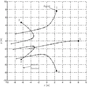
-10 -8 -6 -4 -2 0 2 4 6 8 10 -10 -8 -6 -4 -2 0 2 4 6 8 10 x[m] y [m ] 1 2 3 4 5 Agent desired direction

Figure 2.3: Agents Trajectories with sinusoidal potential for Case I. Each trajec-tory is represented by eighteenth time-steps (each of them has been calculated at the same time t), and there is not any overlapping. For instance, the third sample for agent i2 corresponds to the sixteenth sample for agent i1, whilst the

seventeenth sample for agent i4 is among the first two samples for agent i3.

Considering the sinusoidal control type, the trajectory followed by the agents is shown in Figure 2.3, by which it is possible to observe that there is not any overlapping. In addition, Figure 2.4 well describes this result indicating the relative distances of each agent and the security distance, that it is never overstepped. The velocity components of the agents are plotted in Figure 2.5.

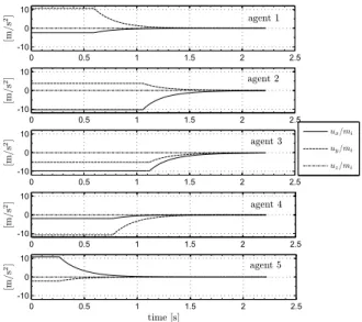
Figure 2.6 shows the temporal history of the three components of the control acceleration ui/mi for the five agents. As we observe in Figure 2.6, during the

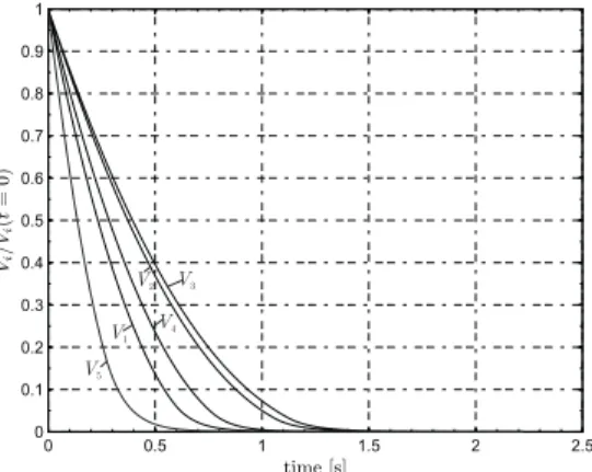
first phase of the manoeuvre the saturation of the control is present due to the high initial velocity of each agent. However, the system converges to the desired condition, as confirmed from Figure 2.7 that shows the temporal history of the total normalized potential (see Eq. (2.9)). In Figure 2.7, we also observe that the function Vi= Vi(t) is a time-decreasing function.

2.5.1 Considerations

We simulated the ability of the swarm for re-aligning by using the three types of repulsive potentials in order to establish which of them well reaches its aim.

(42)

0 0.5 1 1.5 2 2.5 0 2 4 6 8 10 12 14 16 time [s] re la ti ve d is tan ce [m ] 1−2 1−3 1−4 1−5 2−3 2−4 2−5 3−4 3−5 4−5 security distance

Figure 2.4: Relative Distances among agents in Case I. For each agent it is dis-played its distance with all the other agents together with the security distance. According to the resulted trajectory the critical distance is related to the agent

i2 with respect to the agent i3.

In the simulations, we assumed k = 5 that determines the velocity with which the control law follows the desired velocity, as described in Eq. (2.17), therefore the repulsive term in the control law causes a different behaviour of the agents. The scalar function Vi has been built in order to follow the condition

ex-pressed by Eq. (2.4). For this reason, the potential has to be null once the agent velocity vector is aligned with the desired velocity one, and hence the control law provides a command that is proportional to the difference between the cur-rent velocity of the i-th agent vi and the desired velocity v∗ (see Eq. (2.16)).

As a consequence, when the agent is aligned with the desired velocity vector (vi ≡ v∗), the control becomes so small and, therefore, unsensible to the

dis-tinct coming agent and unable to avoid the collision. This inconvenient has been anyway avoided by choosing the right value of the constant kr in the three

dif-ferent cases in order to guarantee the presence of the repulsive factor when the distance between two agents decreases at high rate.

During the simulation we also evaluated the minimum value of the circum-ference radius rmin , where the agents are located, from which the collision is

(43)

0 0.5 1 1.5 2 2.5 -10 0 10 [m / s] vx vy vz 0 0.5 1 1.5 2 2.5 -10 0 10 [m / s] 0 0.5 1 1.5 2 2.5 -10 0 10 [m / s] 0 0.5 1 1.5 2 2.5 -10 0 10 [m /s ] 0 0.5 1 1.5 2 2.5 -10 0 10 time [s] [m / s] agent 1 agent 2 agent 3 agent 4 agent 5

Figure 2.5: Velocity components of the agents in Case I. The final velocity of each agent reaches the desired value v?_{. The vertical and horizontal scales are}

the same for each plot.

0 0.5 1 1.5 2 2.5 -10 0 10 [m /s 2] ux/mi uy/mi uz/mi 0 0.5 1 1.5 2 2.5 -10 0 10 [m/s 2] 0 0.5 1 1.5 2 2.5 -10 0 10 [m/s 2] 0 0.5 1 1.5 2 2.5 -10 0 10 [m /s 2] 0 0.5 1 1.5 2 2.5 -10 0 10 time [s] [m/s 2] agent 1 agent 2 agent 3 agent 4 agent 5

Figure 2.6: Control Effort ui/mi for five agents in Case I. The vertical and

(44)

0 0.5 1 1.5 2 2.5 0 0.1 0.2 0.3 0.4 0.5 0.6 0.7 0.8 0.9 1 time [s] Vi / Vi ( t = 0) V₁ V 5 V 3 V₂ V₄

Figure 2.7: Temporal history of the artificial potential Vifor five agents in Case

I.

Parameter Repulsive potential type gradient gaussian sinusoidal

k 5 5 5

kr 1 1 1

p 1 1 1

tc 1.7896 s 2.5216s 2.5781s rmin 7.4 m 7.6m 7.7m

Table 2.1: Simulation Parameters.

simulations with the convergence time tc and the minimum circle radius rmin.

From Figure 2.1, it is possible to observe that the value of p allows to regulate the velocity with which the value of Vrincreases varying the parameter Dij, and

to avoid the reaching of the saturation level of the control. In addition, in order to determine which control law offers a better behaviour than the others do, several simulations have been done changing the radius of the circle where the agents are located at the beginning of each simulation, determining the value of the minimum radius for which the agents are able to perform their elusive manoeuver without colliding.

In the last analysis, we examined the way in which the performance of the three control laws change by varying the number of agents.

(45)

2.6 Simulations and Results: Case II

Let us consider the case where the final desired velocities have the following components

v?

1= [−5, −1, 0]Tm/s

v?

2= [1, 1, 0]Tm/s

In this case we simulate a swam that reaches a sequence of the desired ve-locities v?

1 and v?2. Considering the sinusoidal control type, the trajectory

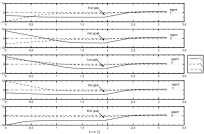
fol-lowed by the agents is shown in Figure 2.8, whereas the velocity components of the agents are plotted in Figure 2.9 and the control acceleration history in Figure 2.10. −10 −5 0 5 10 −10 −8 −6 −4 −2 0 2 4 6 8 10 x[m] y [m ] 1 2 3 4 5 Agent

Figure 2.8: Trajectories followed by the agents in Case II.

2.7 Problem Statement: Extension

In the previous sections it is explained how we found suitable control laws ui(t) in

order to allow the agent i-th to reach the velocity v∗_{and to follow the constraint}

of Eq.2.3. In this section we complicate the initial problem introducing another constraint and changing the artificial potential. The added constraint represents

(46)

0 0.5 1 1.5 2 2.5 3 3.5 −10 0 10 vx vy vz 0 0.5 1 1.5 2 2.5 3 3.5 −10 0 10 0 0.5 1 1.5 2 2.5 3 3.5 −10 0 10 0 0.5 1 1.5 2 2.5 3 3.5 −10 0 10 0 0.5 1 1.5 2 2.5 3 3.5 −10 0 10 time [s] agent 1 agent 2 agent 3 agent 4 agent 5 first goal first goal first goal first goal first goal

Figure 2.9: Velocity components of the agents in Case II. The velocity of each agent reaches the desired values v?

1 and v?2. The vertical and horizontal scales

are the same for each plot.

0 0.5 1 1.5 2 2.5 3 3.5 0 10 20 [m / s ] ux/m uy/m uz/m 0 0.5 1 1.5 2 2.5 3 3.5 −20 0 20 0 0.5 1 1.5 2 2.5 3 3.5 −20 0 20 0 0.5 1 1.5 2 2.5 3 3.5 −20 0 20 0 0.5 1 1.5 2 2.5 3 3.5 0 10 20 time [s] [m /s ] agent 1 agent 2 agent 3 agent 4 agent 5

Figure 2.10: Control Effort ui/mi for five agents in Case II. The vertical and

(47)

the need of each agent to avoid obstacles presented in the scenario where the swarm of agents is located. Imagining to have a set of M obstacles characterized at time t=0 by an initial position xo(0) and a null velocity vo(0) = 0, the new

constraint is expressed as follows:

(xi− xo) · (xi− xo) ≥ b2i (2.43)

where xo is the position of the o-th obstacle closest to the i-th agent with

o = 1, ..., M , kxi− xok is the distance of the i-th agent from the o-th obstacle,

and b2

i is a given constant3. The term bi represents the smallest distance that

has to be observed between the i-th agent and the o-th obstacle.

The changed artificial potential is therefore characterized by the following expression:

Vi= Va(1 + krVr+ koVo) (2.44)

where Vois the obstacle repulsive potential that allows each agent not to collide

with an obstacle, and the term koweights the relative importance of the obstacle

repulsive term with respect to the attractive term.

The first derivative of the potential function Vi expressed by Eq. (2.44) is:

˙

Vi= ˙Va (1 + krVr+ koVo) + krVaV˙r+ koVaV˙o (2.45)

Selecting Eq. (2.12) as artificial potential, and considering Eq. (2.14), after few manipulations, we obtain the control law ui: :

ui mi = ˙vi= − 2 k + kr ˙ Vr+ koV˙o 2 (1 + krVr+ koVo) (vi− v∗) (2.46)

The problem consists of selecting the obstacle repulsive potential Vofunctions

in order to guide the system through the desired final condition without allowing catastrophic collisions among the agents of the swarm and the obstacles. The new term of the artificial potential has to be a simple function of the distance between the i-th agent and the o-th obstacle at each time instant. If we define the parameter Bio as Bio, £ (xi− xo) · (xi− xo) − b2i ¤2 ≥ 0 (2.47)

the distance of the o-th agent closest to the considered i-th agent, is estimated. The continuous, differentiable function Vo = Vo(Bio) has to be chosen in

or-der to satisfy the same conditions expressed for the repulsive potential Vr (see

Eqs. (2.19), (2.20) and (2.21)).

3_{The constant b}2

(48)

Sinusoidal Type

In the section of the repulsive potential we defined a sinusoidal function that contains the advantages of both the gradient type and the gaussian type. The repulsive obstacle potential Vothat can be employed, is expressed by the

follow-ing function: Vo, sin µ π/2 1 + Bs io ¶ (2.48) where s ∈ N+ _{is a positive natural number. Considering the calculations made}

for the repulsive potential of sinusoidal type, the time-derivative of the repulsive obstacle potential of Eq. (2.48) is:

˙ Vo= 2 π s q B_io(2 s−1) (1 + Bs io)2 cos   π/2 1 + Bs io   (xi− xo) · (vo− vi) (2.49)

and the control law ui becomes:

ui

mi

= − nums1+ nums2+ nums3 1 + krsin   π/2 1 + D_ijp   + kosin   π/2 1 + Bs io   (vi− v∗) (2.50) nums1= k (2.51) nums2= kr π p q D(2 p−1)_ij ¡ 1 + Dp_ij¢2 cos   π/2 1 + D_ijp   (xi− xj) · (vj− vi) (2.52) nums3= ko π s q B_io(2 s−1) (1 + Bs io)2 cos   π/2 1 + Bs io   (xi− xj) · (vo− vi) (2.53)

2.7.1 Simulations

Let us consider the case where the final desired velocity has the following com-ponents:

v?= [0, 2, 0]Tm/s

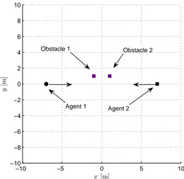
We also take into account a swarm of two agents (N = 2) and the presence of two obstacles (M = 2) in between. We suppose that the first agent is located in front of the second one and the velocity direction of the first agent is against the direction of the other agent (see Figure 2.11). Choosing the parameters ko= 2,

kr= 4, k=6 and s = 2, the swarm is able to reach the desired velocity without

(49)

−10 −5 0 5 10 −10 −8 −6 −4 −2 0 2 4 6 8 10 x[m] y [m ] Obstacle 1 Obstacle 2 Agent 1 _{Agent 2}

Figure 2.11: Initial Scenario Configuration of the agents (at time t = 0). The initial locations of the two agents are i1(−7, 0) and i1(7, 0), whilst the locations

of the two obstacles are io1(−1, 1) and io2(1, 1).

−10 −5 0 5 10 −10 −8 −6 −4 −2 0 2 4 6 8 10 x[m] y [m ] Obstacle Agent 1 Agent 2

(50)

2.8 Conclusions

We proposed a preliminary method for decentralized control of a swarm of ve-hicles using artificial potential method. Two repulsive potentials found in the literature were compared with a proposed sinusoidal approach, and simulations were performed for some scenarios in order to prove the concept. Only the in-formation coming from the closest agent was used in each controller. Simulation also showed the potential capability of dealing with external obstacles. The comparison among the different solutions was performed using the time to reach a desired velocity and how sensitive the swarm is to inter-agent collisions.

(51)

Chapter 3

Conclusions

In this dissertation, artificial potential fields is an effective form for defining swarm-like algorithms. The most important contribution of this dissertation is to show the time needed by swarm to reach a desired velocity and how robust the swarm is to avoid collisions. Three different trial potentials are studied, which satisfy the goals and constraints we stated: 1) swarm obtains a given velocity and 2) does so without internal collisions. In fact, the re-alignment of the swarm in a given direction is achieved by using a decentralized approach, whilst the collision avoidance is obtained by taking into account the different forms of the repulsive potential. In this implementation, the control laws are also able to allow the generic agent to perform an escape manoeuver by using the information related to the state of the closest agent.

The proposed control laws are able to decrease the number of requests for each agent, and in the simplest case only need to know its current and final state. Furthermore, the application of the artificial potential allow us to obtain the analytical control laws, whose expressions are quite simple and compact, enabling an easy on-board implementation with few resources. In the simulation we calculate two metrics to determine which potential is best in a particular situation. The two metrics are: 1) how quickly the swarm converges to the given velocity or equivalently how responsive the swarm is to change in the goal velocity (i.e., tc), and 2) how robust the potential is against collisions (i.e.,

rmin value). Taking into account the results of the performed simulations, we

conclude that the sinusoidal control type produces the best behaviour respect with the other controls.

(52)

3.1 Future Directions

To the authors knowledge, this thesis is one of the studies related to the swarm of UAVs. In this dissertation, we propose a preliminary method for the decentral-ized control of this kind of swarm, defining an artificial potential to determine control laws enabled to allow the swarm to reach his tasks. This method is there-fore far from being complete and exclusive. Several directions can be pursued.

Framework based on artificial potential fields. It could be interesting to design a framework based on artificial potential fields for support different type of collective behaviorus. Doing so, it could be possible to chose the correct potential in order to properly manage group formation, migration and obstacle avoidance of UAVs.

Framework based on UAVs. It could be interesting to design a framework based on UAVs for applying the artificial potential designed in the previous framework and opportunely changed in order to take into account the effective aircraft dynamic model.

(53)

Bibliography

[1] M. Ayre, D. Izzo, and L. Pettazzi. Self assembly in orbit using intelligent components. TAROS, 2005.

[2] J. S. Baras, X. Tan, and P. Hovareshti. Decentralized control of autonomous vehicles. In 42nd IEEE Conference on Decision and Control, pages 1532– 1537, Maui, Hawaii, 2003.

[3] R. H. Battin. An Introduction to the Mathematics and Methods of

Astro-dynamics. AIAA Education Series, 1987.

[4] G. Beni and P. Liang. Pattern reconfiguration in swarms-convergence of a distributed asynchronous and bounded interative algorithm. IEEE Trans.

Robot. Autom., 12:485–490, 1996.

[5] S. Camazine, J.L. Deneubourg, N.R. Francks, J. Sneyd, G. Th´eraulaz, and E. Bonabeau. Self-Organized Biological Superstructures. Princeton, NJ: Princeton University Press, 1998.

[6] J. H. Chuang and N. Ahuja. An analytically tractable potential field model of free space and its application in obstacle avoidance. IEEE Trans. Syst.

Man Cybern., 28:729–736, 1998.

[7] H. K. Dong, O. W. Hua, Y. Guohua, and S. Seiichi. Decentralized control of autonomous swarm systems using artificial potential functions: Analytical design guidelines. Atlantis, Paradise Island, December 14–17 2004. 43rd IEEE Conference on Decision and Control.

[8] D. Dudenhoeffer and M. Jones. A formation behavior for large-scale micro-robot force deployment. pages 972–982. Proc. of the 2000 Winter Simulation Conf., 2000.

[9] V. Gazi. Swarm aggregations using artificial potentials and sliding mode control. IEEE Transactions on Robotics and Automation, 21(6):1208–1214, 2005.

[10] V. Gazi and K. M. Passino. A class of attraction/repulsion functions for stable swarms aggregations. pages 2842–2847, Las Vegas (NV), 2002. Proc. Conf. Decision Contr.

(54)

[11] V. Gazi and K. M. Passino. Stability analysis of swarms. IEEE Trans. on

Automatic Control, 48(4):692–697, April 2003.

[12] S.S. Ge and Y. J. Cui. New potential functions for mobile robot path planning. IEEE Trans. Robot. Autom., 16(3):615–620, 2000.

[13] J. M. Grasmeyer and M. T. Keennon. Development of the Black Widow

Micro Air Vehicle. AIAA, 2001.

[14] H. Haken. Synergetics. In Springer-Verlag, Berlin, 1983.

[15] D. M. Hart. Reducing swarming theory to practice for uav control. pages 3050–3063. IEEE Aerospace Conference Proceedings, 2004.

[16] D. A. Holway, L. Lach, A. V. Suarez, N. D. Tsutsui, and J. T. Case. The causes and consequences of ant invasions. Annual review of ecology and

systematics, 33:181–233, 2002.

[17] D. Izzo and L. Petazzi. Autonomous and distributed motion planning for satellite swarm. Guidance, Control, and Dynamics, 30(2):449–459, March-April 2007.

[18] D. Izzo and L. Pettazzi. Equilibrium shaping: Distributed motion planning for satellite swarm. Munich, Germany, 5–9 September 2005. 8th Interna-tional Symposium on Artificial Intelligence, Robotics and Automation in space - iSAIRAS.

[19] B. H. Krogh. A generalized potential field approach to obstacle avoidance control. In SME Conference on Robotics Research, August 1984.

[20] Yang Liu and Kevin M. Passino. Swarm intelligence: Literature overview. Technical report, Dept. of Electrical Engineering, The Ohio State Univer-sity, March 2000.

[21] P.D. Jr. Lowman. Exploring Space, Exploring Earth. Cambridge: Cam-bridge University Press., 2002.

[22] R. C. Michelson and M. A. Naqvi. Beyond biologically-inspired insect flight. Rto/avt lecture series on low reynolds number aerodynamics on aircraft including applications in emerging uav technology, von Karman Institute for Fluid Dynamics, Brussels, Belgium, 2003.

[23] R. Olfati-Saber and R. M. Murray. Distributed cooperative control of mul-tiple vehicle formations using structural potential functions. Barcelona (Spain), July 21–26 2002. 15th IFAC World Congress.

[24] M. Pachter and P. Chandler. Challenges of autonomous control. IEEE

Control Systems Magazine, pages 92–97, 1998.

[25] H. V. D. Parunak. Go to the ant: Engineering principles from natural multi-agent systems. Altarum Institute, Annals of Operations Research 75, 75:69–101, 1997.

Decentralized Control of a Swarm of Unmanned Aerial Vehicles