Modelling and Analysing Risk at Organizational Level

Modelling and Analysing Risk

at Organizational Level

Yudistira Asnar and Paolo Giorgini

September 2006

Modelling and Analysing Risk at Organizational

Level

Yudistira Asnar and Paolo Giorgini

Department of Information and Communication Technology University of Trento, Italy

yudis.asnar,paolo.giorgini@dit.unitn.it

Abstract. Modeling and analyzing risk is one of the most critical ac-tivity in system engineering and approaches like Fault Tree Analysis, Event Tree Analysis, Failure Modes and Criticality Analysis have been proposed in literature. All these approaches focus on the system-to-be without considering the impact of the associated risks to the organiza-tion where the system will operate. On the other hand, the tendency is more and more to consider software development as a part of organiza-tional development. In this paper, we propose a framework to model and reason about risk at organizational level, namely considering the system-to-be along the organizational setting. The framework extends Tropos, a methodology that has been proved effective in modeling strategic inter-ests of the stakeholders at organizational level. We introduce a number of different means that help the analyst to identify and enumerate relevant treatments for risk mitigation. Experimental results are finally presented and discussed.

1

Introduction

Software systems are more and more part of our life (look how many computers and electronic gadgets are around you), and very often this introduces a broad and strong influence of software in our daily life decisions. The tendency is to consider them as integral and active part of the environment and for this their development has to be considered as part of the social-network development. In this direction, some software engineering methodologies have been introduced (e.g., Tropos [1] and KAOS [2]) to capture since the early phases of the software development the relationships between the software-to-be and the organizational setting. In this new scenario, traditional techniques for modeling and analyzing risk (e.g., Fault Tree Analysis (FTA) [3], Event Tree Analysis (ETA) [3], Failure Mode Effect and Criticality Analysis (FMECA) [4]) have to be reconsidered to extend the analysis to the organization in which the system-to-be will operate. Probabilistic Risk Assessment (PRA) [5] assesses a risk answering to three basic questions: (1) what can go wrong? (2) how likely is it? and (3) what are the consequences? Those traditional techniques are commonly used in Reliability and Safety community, but unfortunately these techniques are not thought to

model the risks at organizational level and they mainly focus on the risks at the system level.

We already have proposed a modeling and reasoning framework to consider risk (more in general uncertain event) at organizational level [6]. The framework extends the Tropos goal models [7, 8] proposing a three layers analysis (i.e., goal, event, and treatment) and algorithms for qualitative reasoning. Section 2 summarizes briefly the framework. In this paper, we extended and refine the framework proposing new types of relationship (modification relation) that allow us to model and analyze circumstances where a countermeasure mitigates a risk reducing its impact and not only the likelihood. Along these relationships, we will introduce new axioms, a refinement of the risk analysis process, and novel reasoning mechanisms (Section 3). We, also, define new types of mitigation actions that can be applied as a part of the solution and we define the guidelines to choose and model them ( 4). We conclude the paper with some experimental results (Section 5) and a final discussion (Section 6).

2

Tropos Goal-Risk Analysis

Tropos has proposed a formal framework to refine stakeholders’ goals and end up with elicits the requirements. The framework can also model the existence of uncertain events, mainly risks, that could give influence to the fulfilment of the goals and treatments that need to be taken to manage the effect of risks. There are three entities that construct goal models, namely Goal, Event (e.g., risk, opportunity), and Treatment (e.g., tasks, countermeasure). Goal analysis results in a number of goal models represented as a graph hG, Ri, where G are nodes (i.e., goals, events, and treatments) and R are relations (decomposition or contribution relations) among them. If (N1, . . . , Nn)7−→ N is one of the noder

relations in R , N1,. . . , Nn are called as the source nodes and N is the target

node of relation r.

Each node has two attributes SAT- Sat(N) and DEN- Den(N) and N ∈ {G, E, T}, which quantify the value of evidence for node being satisfied and de-nied, respectively. Those attributes are indicated as node label and are repre-sented by 6 different satisfaction predicates:

– F S(N), F D(N): there is (at least) f ull evidence that goal G is satisfied (or denied), event E occurs, or treatment T succeeds;

– F S(N), P D(N): there is (at least) partial evidence that goal G is satisfied (or denied), event E occurs, or treatment T succeeds;

– N S(N), N D(N): there is none evidence that goal G is satisfied (or denied), event E occurs, or treatment T succeeds. Actually, they are the same with T predicate in [9]. It is not mandatory to write these predicates in formalization; they could leave implicitly.

The predicates state that there is at least a given level of evidence for the node achievement, and it implies that F S(N) ≥ P S(N) ≥ N S(N) and F D(N) ≥ P D(N) ≥ N D(N), with intended meaning x ≥ y ↔ x → y. .

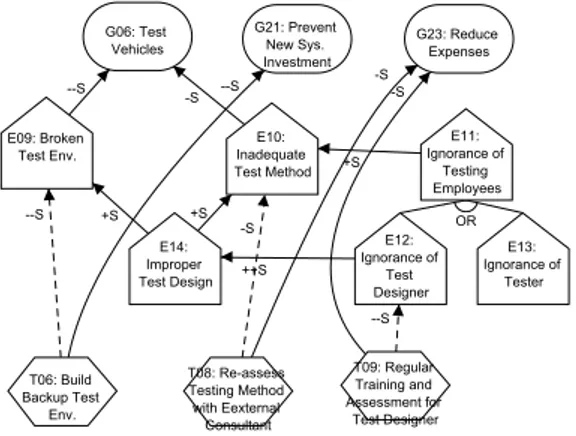
Fig. 1. Part of Goal Model for the Vehicle Production Department

Each entity has separate layer of analysis (see Fig. 1. And each entity can be analyzed using the relations (e.g., decompositions and contributions). Qualita-tive goal analysis in Tropos starts with a number of stakeholders’ goals (called top goals) and each of them is refined by decomposition (AND or OR) into subgoals.

For example, consider to model the strategic objectives of reduce labor costs (G8) is OR-decomposed into reduce man-power by machine (G13) and reduce

salaries (G4). This decomposition and refinements will continue until the goals

are not considered tangible goals, i.e., when there is an actor that can fulfill the goal.

After analyzing the goal layer, we continue to analyze the relevant event that could influence the fulfillment of the goal in goal layer. We define an event as an uncertain circumstance that could influence to the fulfillment of goals [6]. Events can be identified applying different approaches (e.g., obstacle analysis in KAOS [10], Taxonomy-base risk identification [11], or Risk in Finance [12]). Af-terwards, an event is analyzed by a decomposition relation into sub-events until each leaf event can be considered as an independent event. In our framework, a risk is defined as an uncertain event with negative impact and an opportu-nity with positive impact. We represent likelihood by the level of evidence that supports and prevents the occurrence of the event (SATandDEN), and the level of influence of an event is encoded as the type of contribution relation between event and goal. Since the effect of an event obstructs a goal only when it occurs (i.e., denial of an event does not give any impacts), in our model we use only rS

relations, i.e., ++S, +S, −S, and −−S, between an event and goals.

An event can influence more than one goal. For example, in Fig. 1 the event strike (E5) obstructs the satisfaction of reducing salaries (G14) because in this

circumstance labors can demand an increment of the salary. On the other hand, it also obstructs the goal improve production chain (G5) since it can compromise

goals and at the same time as an opportunity for other goals. For instance, the event have a new competitor (E7) is a risk that obstructs the achievement of

the goal high specialized labour (G15) because the competitor can offer better

conditions to the labor. However, the event can also be seen as an opportunity for the goal improve work environment (G12), because it gives more motivations to

the employees to compete with other companies. Event refinement will continue until leaf-events are assessable (i.e., we can assess the likelihood of leaf-event) and the modeler needs to ensure each leaf-event is mutually exclusive.

Once the events have been analyzed, the modeler identifies and analyzes the countermeasures to be adopted in order to mitigate the risks. The mitigation of a risk can be realized in two different ways: reducing the likelihood or reducing the impact. However in our previous work [6], we did not support the mitigation with reducing the impact of risk. In next section, we explain how to model this type of mitigation in Tropos goal model.

Similarly to goals and events, for countermeasures we useSAT and DEN to represent the evidence that supports and prevents the action. A countermeasure has effect on the event layer, and in particular over risks. We represent the effect of a countermeasure as a relation, where its strength is expressed by the type of contribution relations. As for events, we are interested to the propagation of the evidence for the success of a countermeasure (SAT) and therefore we limit the relations between countermeasures and events to rS relations. A countermeasure

mitigates a risk when it adds (propagates) evidence for its denial.

In our model we also allow for relations between the treatment layer and the goal layer. This is useful to model situations where a countermeasure adopted to mitigate a risk has also a contribution (especially negative) to some goals. For instance in Fig. 1, the countermeasure create a labor association (T2) can

mitigate the likelihood of the event strike (E5) – of course this is not always true.

However, the association can have a better bargaining power w.r.t. the individual worker and obtain an increment of the salaries. This produces a negative effect on the satisfaction of the goal reduce salaries (G14).

After finish building the model, we can start analyzing the model and elicit-ing the most reasonable solution to fulfill the stakeholders’ goals. The solution consists of the leaf goals that need to be fulfilled, the treatments that need to be employed to manage the risks of the model and the total cost (leaf goals and treatments). The detail explanation of each step can be seen in [6].

3

Modification Relation in Goal-Risk Model

In previous work, we realize a possibility that a countermeasure mitigate the risk by reducing its impacts, which was not supported, besides reducing the likelihood. This paper will extent Tropos Goal-Risk Model to model it by intro-ducing modification relation. The basic idea of this relation is adding evidence s.t. changes the type of contribution relations.

Modification relation is defined as a relation from Treatment-T to the contri-bution link:

T rS

7−→ r

r is the type of contribution link, and rS is the types of modification relation

(i.e., ++S,+S,−−S,−S). The difference semantics of modification relations can

be seen at its axioms at Fig. 2. In new axiomatization, we can see new symbol (i.e., ∅) for contribution relation. It means the contribution relation does not deliver any evidence to the target node. For instance (Axiom 2), it states that in −−S modification relation, once treatment T has f ull evidence being satisfied,

it will nullify (∅) the target contribution relation (i.e., before is −− relation).

Treatment Invariant Axioms

T : F S(T ) → P S(T ) (1) Treatment to cont. rel. Relation Axioms

T−−S7−→ [−−7−→] : F S(T) → [7−→]∅ (2) P S(T) → [7−→]− (3) T−−S7−→ [7−→] :++ F S(T) → [7−→]∅ (4) P S(T) → [7−→]+ (5) T−−S7−→ [7−→]− _ T−−S7−→ [7−→] :+ P S(T) → [7−→]∅ (6) T−S7−→ [−−7−→] : F S(T) → [7−→]− (7) T−S7−→ [7−→] :++ F S(T) → [7−→]+ (8) T−S7−→ [7−→] :− F S(T) → [7−→]∅ (9) T−S7−→ [7−→] :+ F S(T) → [7−→]∅ (10) T+S7−→ [7−→] :− F S(T) → [−−7−→] (11) T+S7−→ [7−→] :+ F S(T) → [++7−→] (12) T++S7−→ [7−→] :− P S(T) → [−−7−→] (13) T++S7−→ [7−→] :+ P S(T) → [++7−→] (14)

Fig. 2. Basic Axioms of Modification Relations

As an example the treatment manage oil supply (T1) does not reduce the

likelihood of the risk oil price raise (E1) (as we model before in [6]). The correct

modeling way of that circumstance is the T1 mitigates E1 by reducing the

impact of oil price raise to the goal (see Fig. 3(a)). If we assume T3has evidence

f ull of being succeeded then the initial model (Fig. 3(a)) evolves becoming to another model in Fig 3(b) based on Axiom 7.

Finally, we can categorize the treatment into two classes based on its influ-ence: evidence treatment (i.e., a treatment that changes the value of evidence of target node) and effect treatment (i.e., a treatment that changes the type of con-tribution relation). A treatment can occupy both classes. The effect treatment is

(a) initial model (b) final model Fig. 3. Modification Relation

preferable while an event has both impacts (positive and negative), because by means of this treatment we can reduce only the negative impact instead both of them. If we use evidence treatment on this circumstance, then we will lose also the opportunity besides reducing the risk.

3.1 Analysis Mechanisms

The new axioms that have been introduced in previous section, causes a change on the model itself instead changes only the values of model. This fact results an adjustment to the risk analysis steps and several algorithms need to be in-troduced to reason on the new goal model. In the new framework, we can do the similar analysis that has been performed in previous work [6]. We refine the steps of how a modeler performs analysis on the goal model with considering related risks and countermeasures and eliciting the set of optimal solution in Al-gorithm 1. This framework is aiming to support modeller to explore the possible alternative and calculate the defined parameters (e.g., number of SAT andDEN

evidence and the cost of alternative solution), and the decision should be taken manually (i.e., either by modeler or stakeholder).

The Algorithm 1, basically, is alike with the previous one [6] and the only different is Adjust M odel in line 5. Basically, the analysis process consists of the following two steps:

1. find the alternative solutions (line 2-3); 2. evaluate each alternative (line 4-19);

(a) adjust the goal mode based on the evaluated alternative (line 5); (b) assess the risks obstruction to the goal layer (line 9-11);

(c) assess the countermeasures effectiveness to mitigate the risks (line 12-17).

The process starts taking in an input the goal model and a set of desired val-ues for top goals (i.e., satisfaction valval-ues-SAT and acceptable risk values-DEN), and a number of goals as possible candidates for the final solution (input goals). Then Backward Reasoning [8] (line 2) elicits a set of possible assignment values for the input goals such that satisfies the desired values. The modeler chooses a

Algorithm 1 Risk Analysis Process

Ensure: analyse risk for each alternative solutions and find necessary countermeasures to ensure the satisfaction of top goals.

Require: goal model hG, Ri, label array top goals, node array input goals, label array events

1:solution array solution {solution that has already encompassed risks and necessary countermea-sures}

2:alt solution ←Backward Reasoning(hG, Ri, nil, top goals, input goals)

3:candidate solution ←Select Can Solution(alt solution)

{candidate solution ⊆ alt solution}

4:for all Si∈ candidate solution do

5: hG, R0_{i ←Adjust M odelhG, Ri{propagates all modification relations to all related}

contribu-tion relacontribu-tions}

6: if Satisf y(hG, R0_{i, top goals, hS}

i, events, nili) then

7: add(solution,hSi, nill, Calc Cost(Si, nil)i)

8: else

9: boolean array Related Goals ←Related Goals(hG, R0_{i, S} i)

10: labels ←Standard F orward Reasoning(hG, R0_{i, S} i)

11: acc events ←Calc Event(labels, related goals, events)

12: nec treatment ←Backward Reasoning(hG, R0_{i, events, acc events, avail treatment)}

13: for all Tj∈ nec treatment do

14: if Satisf y(hG, R0_{i, top goals, hS}

i, events, Tji) then

15: add(solution,hSi, Tj, Calc Cost(Si, Tj)i)

16: end if

17: end for

18: end if

19: end for

subset of the alternatives on the basis of a certain criteria (e.g., minimum-cost [8], softgoals) called candidate solution (line 3). The rest of analysis process will be limited to this subset. Each candidate solution is now evaluated against risks and then necessary countermeasures are introduced (line 4-19). Before start eval-uating the goal model, we need to adjust model (line 5) by following Algorithm 2 (i.e., it applies all the effects of modification relations). Then, the modeller checks whether the candidate solution in adjusted model needs countermeasures to ob-tain the desired values in the top goals. If not the candidate solution is added directly to the solution and its cost is calculated (line 7). Otherwise, counter-measures must be introduced in the candidate solution (line 9-17).

For applying modification relation, we perform Algorithm 2 with taking in hG, Ri as initial goal model and a set of initial values of input goals. The Algo-rithm 2 will modify the model (i.e., strictly speaking R) until the model stable (line 5), i.e., no change anymore, in terms of the relation in goal model and the final values. First step is doing N ew F orward Reasoning [6] to gain the final evidence values of all nodes in the model (in this step, modification re-lations are not considered). Based on the those values, we apply modification relations on the initial model hG, Ri by changing the type of all related contri-bution relations following U pdate Relation (Algorithm 3) and results the new model hG, R0_{i. U pdate Relation basically calculates all the impacts of}

modifica-tion relamodifica-tions over a particular contribumodifica-tion relamodifica-tion. Apply Rules M odif y Rel is a function to define the effect of a modification relation over a contribution relation, that is underlain by the axioms in Fig. 2. If a contribution relation relates with several modification relations, we will take the worst possible mod-ification. For that purpose, we define the order of contribution relation types:

−− ¿ − ¿ ∅ and ∅ ¿ + ¿ ++, with intended meaning −− is worse than − and respectively for others. This principle (in line (5) and (7)) intends to make the organization be prepared with the worst condition.

Algorithm 2 Adjust Model

Ensure: Adjust Goal Model (Attribute values and Relation Types) Require: goal model hG, Ri, label array init val

1:goal model cur model, old model

2:label array cur val

3:cur model ←hG, Ri

4:cur val ←init val

5:while old model 6= cur model and old value 6= cur model do

6: old model ←cur model

7: old value ←cur value

8: cur value ←N ew F orward Reasoning(cur model, init val)

9: for all Ri∈ R s.t. ∃Rel ∈ R : target(Rel) = Rido

10: cur model.R[i] ←U pdate Relation(i, init model, cur val)

11: end for

12: end while

13: N ormalize M odel(cur model){Pruning relation (R) s.t. R = [7−→] or target(R) = [∅ 7−→]}r

14: return cur model

Algorithm 3 Update Relation

Ensure: Change the type of contribution in goal model Require: int i, goal model hG, Ri, label array value

1:for all Rj∈ R s.t. target(Rj) = hG, Ri.Rido

2: arcj ←Apply Rules M odif y Rel(Rj, value)

3:end for

4:if Is N egative(old.model.R[i]) then {the type is risk relation i.e., “− or −−”}

5: rel type ←M ax Array(arc)

6:else {opportunity relation i.e., “+ or ++”}

7: rel type ←M in Array(arc)

8:end if

9:return rel type

4

Alternative Solution of Risks in Goal-Risk Model

After extending the goal model to coup with all possible behavior of a treatment (e.g., by changing the evidence value of target nodes or by changing the impact of contribution relation). This paper will also explain the guidelines for a modeler while facing the risks in order to manage them such that acceptable for the fulfillment of stakeholders’ goals.

Basically, there are two way that could be taken while we have a risk in our organization, the first is trying to find other alternative s.t there is no risk related with it and the other is mitigating the risk s.t. it is acceptable. Once the modelers decide to elicit a treatment to mitigate a risks, they need to be aware with the effects to other entities (i.e., goal, event, treatment).

We categorize treatments into 5 types of measure that can be used to over-come the risk: avoidance, prevention, alleviation, detection, and retention. The order of the types can be seen also as the steps in eliciting the treatments. First, the modelers try to find the way to avoid the risks, if it is not possible then they should try to prevent the occurrence the risks. If the prevention measures are not adequate then try to identify the alleviation measures. If it is also not ade-quate, then they need to identify the detection measures otherwise they should be ready with any retention measures.

The next passage will detailed them by specifying what are the model char-acteristics that can lead in choosing the proper type of measures and what is the consequences (advantage and disadvantage) of each type. However, the model characteristics are defined, as follow:

– for goal (i.e., is defined as leaf goal in goal layer): the importance of the goal and its fulfillment type (i.e., achieve goal, maintain goal, and achieve-maintain goal [13]);

– for event (i.e., is defined as top event in event layer): the impacts and likeli-hood of the event, the structure of event tree in event layer, and the type of risks (e.g., avoidable, preventable, reduceable);

– for treatment (i.e., is defined as leaf treatment in treatment layer), the success rate in mitigating the risks, the cost of the treatment.

4.1 Avoidance

It defines as an activity that tries to achieve the stakeholders’ goals by choosing an alternative in which there is no risks related to it.

Model characteristic for this type is the goal fulfillment is very important for the stakeholders and most of the time, the goal is categorized as a maintain goal or an achieve-maintain goal. Thus, the modeler should ensure its fulfilment all the time. However, this type of measures is not always possible to be elicited, there is a circumstance in which the modeler do not have any alternatives to fulfill the goal with risk free. For example in Fig. 4, the modeler can fulfill G8 by means

of choosing G13 or G14. In this scenario, the modeler choose G13 instead

of G14 because G8 must be fulfilled all over the time.

Consequence of this type is no need to introduce any treatments that possibly give bad impacts to the goal layer besides the good ones. The only possible drawback of this type is the risk-free alternative could be more costly than the total cost risky alternative and its treatments. Therefore, there is a possibility which the cost of G13 is higher than the cost G14 and its treatment (e.g.,

T2).

4.2 Prevention

This activity demands the modeler to elicit any treatments that can prevent the occurrence of the negative event. The notion of prevent means reduce the risk until acceptable value for fulfillment of stakeholders’ goals.

Fig. 5. Prevention Means

Model characteristic that suits for this type is the risk obstructs significantly the stakeholders’ goals and unavoidable. This type of measures are carried on by reducing the likelihood of related leaf-events s.t. the likelihood of the top-event is also reduced. To identify the related leaf-events, we can use the same technique that commonly used in defining minimal cut-set in FTA [3]. For instance (in

Fig. 5), build back up test environment (T6) is a measure that dedicated to

elim-inate the possibility of unavailability of testing environment because of broken test environment (E9) occurs. This type is less economic while meets the risk

with many alternatives of occurrence (or-decomposition), because the risk will be really reduced when we prevent all the leaf-events of the risk. For instance, Regular Training and Assessment for Test Designer (T9) is not really effective

to reduce the ignorance of testing employees (E11) because it could be caused

of the ignorance of tester (E13).

Consequence of this approach is it can not guarantee 100% risk-free of the model, differently with avoidance measure, because there is a chance that the treatment is failled to mitigate the risk. The cost of prevention measure is certain whether the risk occurs or not. Therefore, this type is not suited to mitigate the risk with very low likelihood.

4.3 Alleviation

This measure intends to reduce the effect of risk to goal layer by employing effect treatment in proper place (i.e., the impact relation between top event and goal).

Fig. 6. Alleviation Means

Model characteristic for this type is if the modeler can not find the way to avoid or prevent the risk. For instance (in Fig. 6), oil price raise (E1) can be caused

by oil stock manipulation (E2) or gulf war (E3). The vehicle company does

not have capability to reduce the likelihood of both events therefore the only possible thing to do is to mitigate s.t. the impact of E1 is less harm to the

goal layer. Besides that, this type is suited for the circumstance which there are so many leaf-events need to be mitigated in order to prevent a top event s.t. the total cost of mitigation action of the risk is not economic as we mention in prevention measure.

Consequence of having un-mitigated risk will follow the success rate of treat-ment in alleviating. Therefore, this measure is recommended to be applied if the modeler is really sure it can reduce the impact of the risk otherwise the organi-zation will suffer an un-mitigate risk. The probability of spending budget to do this action will follow the likelihood of top event/risk and the likelihood of top event is always less or equal than all its sub-events. Thus, it is very suitable for the unlikely risks.

4.4 Detection

A treatment mitigates a intermediate event in event tree s.t. it reduces the risk. In this circumstance, actually the failure has occurred within the organization but the impacts of risk have not delivered yet to the goal layer.

Model characteristic for this type is once the modeler can not find mitigation action with previous types. Moreover, this type will reduce the cost of treatment if several events/risks share their sub-tree, because the treatment can mitigate the overlapped sub-tree and it will reduce all the risks at the end. Typically, it is done using evidence treatment. For example (in Fig. 7, re-schedule and maintain test environment (T7) will reduce the likelihood of overload test environment

usage (E8), and consequently reduces the possibility of stress condition (E19)

for employees which can obstruct the achievement of the goal to improve work environment condition (G12) and it also reduces the chance of having broken

test environment (E9) that could lead us to the denial of goal to do test vehicle

(G6) properly.

Consequence of this types will be catastrophic if the measure fails to reduce the intermediate event, because it could cause more than one top-event/risk. Therefore, the modeler should be aware of the final consequences if the coun-termeasure fails and how much is the success rate of the councoun-termeasure before choosing this type. The probability of cost of the detection measures follows the likelihood of its intermediate event (i.e., equal or higher than likelihood of top events).

4.5 Retention

It is the last alternative for an organization to deal with its risk, once we can not find any treatments from the previous types. This type of treatment is usually

Fig. 7. Detection Means

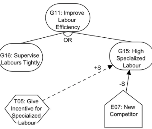
employed when the organization do not have capability to mitigate the risk (e.g., war, inflation, new competitor, natural disaster). For instance (in Fig. 8), the risk of having new competitor (E7) is beyond the company capabilities and it

could obstruct the goal of having high specialized labor (G15) because they can

give better offer to the specialize labor. The only thing that company can do is trying to give incentive for specialized labor (T5) s.t. the achievement of G15 is

maintained. Transfer the risk to an insurance company, restore the obstructed goals, and design fault tolerance system can be categorized in this type. Because they do not reduce the likelihood nor the effects of risks, they just try to make the consequence of the risk is less catastrophic.

Consequence of applying this type is there is a certain period that the goal might be un-satisfied before it is restored. Besides that, this measure can be seen as a mean to fulfill the goal besides only as a treatment for the risk.

5

Experimental Result

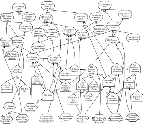
In this section, we briefly present some experimental results of a case study Vehicle Manufacture (in Fig. 9) obtained with the new algorithm and the help

Fig. 8. Retention Means

of an extension tool of the Goal Reasoning Tool1 _{(GR-Tool) developed within}

the Tropos project.

For their implementation we started from the GR-Tool reasoning mechanisms and we have re-implemented them introducing the necessary modifications as described in Section 3. For more details about the GR-Tool and its extension we suggest to visit the Tropos web page.

Suppose we want to obtain a fully satisfaction of all top goals i.e., reducing cost (G1), increasing quality of vehicles (G2), and increasing Return of

Invest-ment(ROI) (G17) with avoid any risks on them. So we have as input { Sat(G1)

=F, Sat(G2) =F, Sat(G17) =F}. Executing Backward Reasoning we find a set

of possible solutions.For the case study, we have 14 alternative solutions (i.e., minimum assignment of input goals s.t. they achieve top goals) as seen in Ta-ble. 1 (we eliminate the input goals that are taken by all alternative). In next passage, we concentrate in analyzing the S1 which are the second cheapest al-ternative. This choice is taken because S13 and S14 are using G14 to fulfill

top goals, i.e., G1 and G17. This manner is too risky because once G14 fail

then there are more than one top goal will follow. Of course, other criteria can be adopted for the selection of the alternative solution to be analyzed.

Table 2 summarizes the label values during the reasoning on S1. Forward reasoning is applied then to calculate the effects of the selected solution to the other goals of the model (column “Goal-Out” Table 2). Now, let suppose we have evidence about the occurrence of some of the events and want to see the impact of them on the goal layer. For example, considering the event assignment reported in column “Event-In” (i.e., Sat(E7, E16, E17) =F and Sat(E2, E6, E12, E13, E14, E18)

=P), we obtain that (“Event-Out”) top goals G1, G2, G17 are partially

denied. In order to re-obtain the desiderata values for top goals we need to find necessary treatments able to mitigate the risks. There are four possible counter-measure sets that could be taken to mitigate the risks (see Table 5) and the total

Fig. 9. Goal Model for the Vehicle Manufacture

cost of countermeasures can be calculated summing up the single cost of input treatments. In this experiment, we adopt C1 based on their costs and their side effects. Even C1 is not the cheapest, it is worth because by choosing T4 instead

T3, T4 gives positive effects to the achievement of G7 (i.e., even it is not one

of the input goals). Finally, the tool generates the final configuration with input S1 and C1 (in column ”Treatment-Out”) where our desired values for top goals are again obtained except G17 (i.e., Den(G17) =P). In this combination (i.e.,

S1 and C1), the effect of E1−−7−→ GS 9is nullified by applying T4 s.t. E17−→∅

G9, and it also the case for E77−→ G−S 15and E147−→ E−S 9.

6

Conclusions

In this paper, we have presented a framework to model and reason about risk within the requirements engineering process. We have adopt and extended the Tropos goal modeling framework and proposed qualitative reasoning algorithms to analyse risk during the process of evaluation and selection of alternatives.

Input Goal Cost S1 S2 S3 S4 S5 S6 S7 S8 S9 S10 S11 S12 S13 S14 G07: Use Raw Materials Efficiently 4 X X X X

G09: Reduce Energy Costs 5 X X X X

G13: Reduce Man-Power by Machine 9 X X X X

G14: Reduce Salaries 8 X X

G15: High Specialized Labour 7 X X X X X X X

G16: Supervise Labours Tightly 7 X X X X X X X

G23: Reduce Expenses 5 X X X X X X

G24: Reduce Tax Payment 5 X X X X X X

Total Cost 16 16 16 16 17 17 17 17 21 21 21 21 15 15

Table 1. Cost of Alternative Solutions

Cost C1 C2 C3 C4

T02: Create Labour Association 6 X X X X

T03: Have Partnership with Oil Company 6 X X

T04: Have Supply Chain Mgmt Sys 8 X X

T05: Give Incentive for Specialized Labour 7 X X X X

T06: Build Backup Test Env. 8 X X

T07: Re-Schedule-Maintain Test Env. 6 X X X X T08: Re-assess Testing Method with Ext. Consultant 5 X X X X T09: Training and Assessment for Test Designer 5 X X X X T10: Have Long Contract for Specialized Labour 6 X X X X

Total Cost 43 51 41 49

However, this work has overcame one limitation of previous work which ,now, it supports relationships between nodes (goals, events, tasks) and can model situations where a treatment mitigates the risk reducing its impact on the goal layer. by introducing the possibility to establish relations also between nodes and arcs.

Besides that, this paper explains several type of measures that typically is used to deal with the existence of risks in the organization. They are categories as: avoidance, prevention, detection, alleviation, and retention. The modeler should understand the model characteristics before choosing them, especially: preven-tion, detecpreven-tion, alleviapreven-tion, and be aware of their consequences. Because avoid-ance is usually chosen if the condition allows, and retention is the last option if there is no other type of measures that suits with the model. Thus, we would emphasize in two consideration points in placing the measures:

– Possibility of spending budget mitigating the risk

P oss(Cost P revention) À P oss(Cost Detection) À P oss(Cost Alleviation) For prevention measure, it is certain that the organization will spend the bud-get for this measures, and detection measure is less than prevention measure but is still greater than the possibility of spending of alleviation measure. – Success rate that is demanded for each type:

Goal Event Treat. In Out In Out Out

S S D S S D S D

E01: Oil Price Raise - - - - P - P

-E02: Oil Stock Manipulation - - - P P - P

-E03: Gulf War - - -

-E04: Increase Minimum Salary Policy - - -

-E05: Strike - - - - P - -

-E06: Increase Unemployment Rate - - - P P - P

-E07: New Competitor - - - F F - F

-E08: Overload Test Env. Usage - - - - F - -

-E09: Broken Test Env. - - - - P - -

-E10: Inadequate Test Method - - - - P - -

-E11: Ignorance of Testing Employees - - - - P - P

-E12: Ignorance of Test Designer - - - P P - - P

E13: Ignorance of Tester - - - P P - P

-E14: Improper Test Design - - - P P - P

-E15: Bad Test Scheduling - - - - P - P

-E16: Heavy-Weight Test Design - - - F F - F

-E17: Tight Testing Schedule - - - F F - F

-E18: Run out resources - - - P P - P

-E19: Stress Situation - - - - P - -

-G01: Reduce Costs - F - - F P F

-G02: Increase Quality of Vehicles - F - - F P F

-G03: Reduce Resources Costs - F - - F P F

-G04: Have Efficient Production System F F - F F - F

-G05: Improve Production Chain - F - - F P F

-G06: Test Vehicles F F - F F P F

-G07: Use Raw Materials Efficiently - - - P

-G08: Reduce Labour Costs - - - - P P P

-G09: Reduce Energy Costs F F - F F P F

-G10: Use Monitoring Mechanism F F - F F - F

-G11: Improve Labour Efficiency - F - - F - F

-G12: Improve Work Environments F F - F F P F

-G13: Reduce Man-Power by Machine - - -

-G14: Reduce Salaries - - P - P P P P

G15: High Specialized Labour F F - F F P F

-G16: Supervise Labours Tightly - P - - P - P

-G17: Increase ROI - F - - F P F P

G18: Reduce Investment Rate - F - - F - F

-G19: Decrease Cost - F - - F - F P

G20: Increase Revenue F F - F F P F P

G21: Prevent New Sys. Investment F F - F F - F

-G22: Selective Investment F F - F F - F

-G23: Reduce Expenses F F - F F - F P

G24: Reduce Tax Payment - - -

-T01: Manage Oil Supply - - - F

-T02: Create Labour Association - - - P

-T03: Have Partnership with Oil Company - - -

-T04: Have Supply Chain Mgmt Sys - - - F

-T05: Give Incentive for Specialized Labour - - - F

-T06: Build Backup Test Env. - - - P - P

T07: Re-Schedule-Maintain Test Env. - - - F

-T08: Re-assess Testing Method with Ext. Consultant - - - F -T09: Training and Assessment for Test Designer - - - F -T10: Have Long Contract for Specialized Labour - - - P -Table 2.SAT-DENvalues in Risk Analysis of S1

Before applying the measure in the model, the modeler should ensure the success rate of the measure in mitigating the risk deploy it in the model. The detection measure is demanded the highest success rate because it will mitigate more than one top-risk, so its failure can cause several obstructions in goal layer. The alleviation measure needs less than detection one but is higher than prevention measure. Because the prevention measure usually works with several others, its effect of failure can be reduced by the others, and it is not the case for the alleviation because one it fails the impact of the risk will deliver to goal layer as it is (i.e., typically, it obstructs only one goal).

Finally, as done for goal models we want to propose also quantitative reason-ing mechanisms where evidence is expressed in term of probability model.

References

1. Bresciani, P., Perini, A., Giorgini, P., Giunchiglia, F., Mylopoulos, J.: Tropos: An Agent-Oriented Software Development Methodology. Autonomous Agents and Multi-Agent Systems 8(3) (2004) 203–236

2. van Lamsweerde, A., Letier, E.: Handling Obstacles in Goal-Oriented Require-ments Engineering. IEEE Transaction Software Engineering 26(10) (2000) 978– 1005

3. Stamatelatos, M., Vesely, W., Dugan, J., Fragola, J., Minarick, J., Railsback, J.: Fault Tree Handbook with Aerospace Applications. NASA (2002)

4. DoD: Military Standard, Procedures for Performing a Failure Mode, Effects, and Critical Analysis (MIL-STD-1692A). U.S. Department of Defense (1980)

5. NASA: Probabilistic Risk Assessment Procedures Guide for NASA Managers and Practitioners. http://www.hq.nasa.gov/office/codeq/ (2002)

6. Asnar, Y., Giorgini, P., Mylopoulos, J.: Risk Modelling and Reasoning in Goal Models. Technical Report DIT-06-008 (Submitted to RE-2006), DIT - University of Trento (2006)

7. Giorgini, P., Mylopoulos, J., Nicchiarelli, E., Sebastiani, R.: Reasoning with Goal Models. In: ER ’02: Proceedings of the 21st International Conference on Concep-tual Modeling, Springer (2002)

8. Giorgini, P., Mylopoulos, J., Sebastiani, R.: Simple and Minimum-Cost Satisfia-bility for Goal Models. In: CAISE ’04: In Proceedings International Conference on Advanced Information Systems Engineering. Volume 3084., Springer (2004) 20–33 9. Giorgini, P., Mylopoulos, J., Nicchiarelli, E., Sebastiani, R.: Formal Reasoning

Techniques for Goal Models. Journal of Data Semantics (2003)

10. van Lamsweerde, A., Letier, E., Darimont, R.: Managing Conflicts in Goal-Driven Requirements Engineering. IEEE Transaction Software Engineering 24(11) (1998) 908–926

11. Carr, M.J., Konda, S.L., Monarch, I., UlrichCarr1993, F.C.: Taxonomy-Based Risk Identification. Technical Report CMU/SEI-93-TR-6, ESC-TR-93-183, Software Engineering Institute, Carnegie Mellon University (1993)

12. Holton, G.A.: Defining Risk. Financial Analyst Journal 60(6) (2004) 1925 13. Fuxman, A., Kazhamiakin, R., Pistore, M., Roveri., M.: Formal Tropos: language