A follow-me algorithm for AR.Drone using MobileNet-SSD and PID control

Faculty of Mathematics and Computer Science

A follow-me algorithm for AR.Drone

using MobileNet-SSD and PID control

Author: Júlia Garriga Ferrer

Director:

Dr. Lluís Garrido

Affiliation: Departament of Applied Mathematics and Analysis

the door to the creation of new applications and technologies. This thesis presents a vision-based autonomous control system for an AR.Drone 2.0. A tracking algorithm is developed using onboard vision systems without relying on additional external inputs. In particular, the tracking algorithm is the combination of a trained MobileNet-SSD object detector and a KCF tracker. The noise induced by the tracker is decreased with a Kalman filter. Furthermore, PID controllers are implemented for the motion control of the quadcopter, which process the output of the tracking algorithm to move the drone to the desired position. The final implementation was tested indoors and the system yields acceptable results.

Introduction vii

Motivation vii

Objectives vii

MobileNet and Single Shot Multibox Detector (SSD) viii

PID control viii

Thesis organization ix

1 Prior knowledge 1

1.1 Computer vision preliminaries 1

1.1.1 Supervised learning and neural networks 1

1.1.2 Object detection 7

1.1.3 Object tracking 12

1.2 Quadcopter control 13

1.2.1 AR.Drone 2.0 13

1.2.2 Available open-source libraries 16

2 Framework overview 17

2.1 Detection and tracking of the person 18

2.2 Kalman filter and error computation 19

2.3 PID controller 23

2.4 Drone movement 24

3 Software implementation 25

3.1 Source code organization 25

3.2 Software explanation in depth 26

3.2.1 Initialization 26 3.2.2 Tracking algorithm 27 4 Results 33 4.1 Tracking robustness 33 4.1.1 Landed quadcopter 33 4.1.2 Quadcopter in motion 35

4.2 Kalman filter evaluation 37

5 Conclusions 43

5.1 Summary and complications 43

5.2 Future work 43

Motivation

Every year the industry of automation and robots is increasing and the business of UAV (Unmanned aerial vehicles) provides less expensive and better models. In particular, quadcopters or, as popu-larly said, drones, are becoming more readily available, smaller and lighter. At the same time, the industry of cameras is also inflating, thanks to applications like Instagram people create images and videos for the sole purpose of sharing them to the social media. Because of this, quadcopters are being used for the creation of spectacular aerial images and videos that could not be made before. But drones with high quality cameras are much more expensive than regular drones. Although now, some of these cheap quadcopters allow a camera to be inserted on top, which makes the overall price less expensive. Another technology that has been booming for two years now is the follow-me drones: quadcopters programmed to automatically follow a target around, giving the opportunity to film unique aerial shots. This technology can be created with the use of a GPS device along with a transmitter, or by using sensors and object recognition on the target. If we combine the follow-me technology, plus the cheap quadcopter, plus an inserted good camera, we get a not very expensive and useful device, that can create high resolution videos while following you around.

The motivation of this project is to create a follow-me quadcopter implementation, able to track a target through daily activities, like running, climbing, swimming, etc. by only using the images obtained from the drone, with the help of computer vision algorithms.

Objectives

The objectives of this thesis are three. First, to implement a tracking algorithm in the three-dimen-sional space from two-dimenthree-dimen-sional video frames, this is, an algorithm able to follow the movement of the person through the height, width and depth planes using consecutive frames from a video. Second, to control an AR.Drone 2.0 so that it follows the observations given by the tracking algo-rithm, creating a follow-me implementation of the AR.Drone 2.0. Third, to run the implementation in a low speed processor: the CPU of a laptop, or even a smartphone or tablet, allowing the target to send, in real time, commands to the quadcopter.

MobileNet and Single Shot Multibox Detector (SSD)

In general, the input of an object tracker is the bounding box containing the object to track. To obtain this bounding box an already trained object detector network can be used. In this case we use an implementation of the MobileNet-SSD detection network.

On one hand, MobileNet, [HZC+17], is an efficient network architecture especially designed for mobile and embedded vision applications. MobileNets are small, low-power, low-latency models effective across a wide range of applications and use cases including object detection, classification, face attributes and large scale geo-localization. The accuracy of MobileNets is surprisingly high and good enough for many applications, although not as good as a full-fledged neural network.

On the other hand, SSD,[LAE+15], is a method for detecting objects using a single deep neural net-work, easy to train and simple to integrate in systems that require a detection component. Moreover, experimental results on the PASCAL VOC, COCO, and ILSVRC datasets show that SSD has competi-tive accuracy to other slower methods. This combination of speed and accuracy make this method a very good option to use for our purpose.

PID control

To accomplish the task of automatic control of an AR.Drone 2.0 a PID controller is required.

The proportional-integral-derivative controller, or PID controller, is the most common type of con-troller used for UAV stabilization and autonomous control. It is a control loop feedback mechanism that attempts to minimize the error between a measured value and a desired value. The three terms: proportional, integral and derivative, compose the controller algorithm and try to minimize this er-ror. The proportional corrects instances of error, the integral corrects accumulation of error, and the derivative corrects the actual error versus the error from the last iteration. To obtain a stable PID controller three parameters related to each of these terms have to be tuned. The goal of tuning is to reach the point right before erratic behaviour, where the quadcopter can get to the desired state quickly but without overshooting or oscillations. The parameters that produce the desired behaviour depend on the dynamics of the system being controlled.

Thesis organization

This essay is organized in five chapters:

• Chapter 1 explains the preliminaries needed to start with this project. First, it explains the different state of the art object detectors and object trackers, starting with an introduction to neural networks. Second, it talks about the quadcopter chosen for the project: the AR Drone 2.0, and the different methods that exist to create a communication with this quadcopter. • Chapter 2 gives an in depth explanation of the project’s framework, mostly theoretical without

entering in the coded software. It introduces the Kalman filter for smoothing the tracking output and the PID controller for the control of the quadcopter.

• Chapter 3 describes, given the theoretical framework from Chapter 2, the implementation of the tracking and moving algorithms.

• Chapter 4 shows the results obtained of the implementation. • Chapter 5 concludes the thesis and talks about future work.

The desired quadcopter behaviour is achieved by the interaction of two separate modules which provide two different functionalities: the tracking of the person on one hand, and the actual control logic of the quadcopter on the other. For the first task an object detection system is needed in order to find the person in the first frame right after the drone startup, and a tracking system is needed in order to follow this detected target. For the second task a control API can be made from scratch using the quadcopter low-level commands, or an existing, off-the-shelf and ready-to-use library can be used. The goal of this chapter is to provide a succinct introduction to the topics that have to be addressed in order to implement a solution for both tasks, and at the same time, to review the most relevant approaches to date and decide which are the most convenient for this thesis.

1.1

Computer vision preliminaries

The problem of human detection (embedded in the general problem of object detection) is the prob-lem of automatically locating people in an image or video sequence, the latter case is usually referred to object tracking. When dealing with a video feed, there are two approaches to locate the interest object in each frame. On the one hand an object detector can be queried on every frame, so that the video sequence object tracking is effectively reduced to multiple independent (per-frame) detec-tions. On the other hand a time-aware system can be used so that prior information from past frames is exploited to infer the object location in the current frame. A memoryless approach such as the former is usually more computationally expensive because the object location must be determined every time from scratch, while the latter approach tends to be faster but less accurate because the prior information alone (such as the previous object location) has to be corrected by some ad hoc hypothesis or model, which tends to produce drifted predicted locations. In this section we will focus on the general problem of object detection and tracking, starting with a brief explanation of how do supervised learning and neural networks work, which will help us understand the now state of the art object detection systems.

1.1.1

Supervised learning and neural networks

Supervised learning is a statistical subject which provides the mathematical setting to learn from example. Specifically, one has a set of training samples

drawn from the joint unknown distribution

f: Rn× Rm−→ [0, 1] which models a stochastic function

h: Rn−→ Rm

x_{7−→ y = h(x)} (1.1)

Given a parametric model

ˆh: Rn

× Rk−→ Rm (x, ψ) 7−→ ˆh(x, ψ) and a cost function

L: Rm× Rm−→ R (a, b) 7−→ L(a, b) the goal of supervised learning is to find

ˆ ψ = arg min ψ N X i=1 L(ˆh(xi,ψ), yi) (1.2)

so that ˆh(·, ˆψ) is a good approximation of h. Supervised learning can be divided into two categories: • Classification problems: discrete output, it includes models such as Support Vector Machines,

Artificial Neural Networks and Naïve Bayes classifiers.

• Regression problems: continuous output, it includes models such as Linear Regressors, Deci-sion Trees and Artificial Neural Networks.

Since Artificial Neural Networks currently provide state-of-the-art results in supervised learning tasks we will stick to these models.

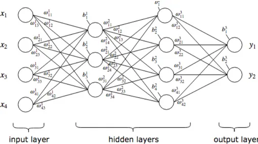
Artificial neural networks are a brain-inspired system intended to replicate the way the human brain works. They consists in a collection of interconnected units or nodes called artificial neurons that can transmit signals from one to another and operate in parallel according to the given input. Depending on their inputs and outputs, these neurons are generally arranged into three different layers (fig 1.1):

• Input layer: dimensioned according to the input. • Hidden layer(s).

Depending on the connectivity between the neurons in the hidden layer(s) the neural network can be a feed-forward network, where the information travels in one direction, from input to output, or a feedback network, where the information can travel in both directions.

Neural networks can also be used for unsupervised learning (e.g. autoencoders,[Bal12]), but our focus will be on the supervised neural networks, which are the most common. From now on, when referring to neural networks we will be talking of supervised neural networks. As neural networks are a type of supervised learning method they will have a training dataset, a parametric function (which is the neural network) and a cost function, as explained above, and their goal will be to find theψ that meets (1.2). This ψ is a k-dimensional vector and their ψ₁, ..,ψ_k components are called weights,ω, and biases, b. A basic neural network with no hidden layers is

ˆh_i=

n

X

j=1

ωjixj+ bi i= 1, ..., m; bi,ωi j, xj∈ R

whereω_{i j}’s are the weights and b_i’s are the biases, so thatω_{i j}, b_{i∈ {ψ1}, ..,ψ_k}.

In figure 1.1 we have an example of a neural network with two hidden layers of dimensions 3 and 4, with all the corresponding weights and biases.

Let M_lbe the matrix formed by all the weights from layer l_{−1 of dimension v to layer l of dimension} u: M_l=            ωl 11 ωl21 · · · ω_(v−1)1l ωlv1 ωl 12 ωl22 · · · ω_(v−1)2l ωlv2 .. . ... ... ... ... ωl

1(u−1) ωl2(u−1) · · · ωl(v−1)(u−1) ωlv(u−1)

ωl 1u ω l 2u · · · ω l (v−1)u ωlvu            ,

So that with no hidden layers we have:

ˆh = M x + b, (1.3)

with x_{∈ R}n_{, b∈ R}m_{, M= M}

1∈ Rm×n.

If we had one hidden layer of dimension d our output would be:

ˆh = M2(M1x1+ b1) + b2= (M2M1)x + (M2b1+ b2) = M x + b, (1.4) with b1∈ Rd_{, b}2

∈ Rm_{, M}

1∈ Rd×n, M2∈ Rm×d.

Equation (1.4) shows that, with this network architecture, and even by adding additional hidden layers, the only functions that our network will learn are going to be linear functions. To be able to approximate nonlinear functions we need (non-linear) activation functions. For example, if our net-work is used to know if tomorrow is going to rain (output 1 if so, 0 if not) we could write something like this: ˆh_i =    0 i f Pn_j=1ω_{i j}x_j≤ ξi 1 i f Pn_j=1ωi jxj> ξi i= 1, ..., m ξi,ωi j, xj∈ R

In this case, the activation function used is called the threshold function, which generates the output 1 if the input exceeds a certain valueξ_i = −b_i. This type of neural networks that performs binary classification are called perceptrons.

But perceptrons are not continous (a small change in the input may produce a large change in the output), therefore expression (1.2) cannot be solved using standard analysis techniques. To fix this, other activation functions, which are differentiable, are used. For example the sigmoid function:

σ(x) = 1

1+ e−x ∈ (0, 1) which applied to our neural network would be:

ˆh_i= 1

1+ ex p(− Pn_j=1ω_{i j}x_j− bi)

i= 1, ..., m b_i,ω_{i j}, x_j∈ R, the hyperbolic tangent function:

so that ˆh_i = tanh n X j=1 ωi jxj+ bi ! i= 1, ..., m b_i,ω_{i j}, x_j∈ R or the Rectified Linear Unit (ReLu) function:

f(x) = max(0, x) so that ˆh_i= max(0, n X j=1 ωi jxj+ bi) i= 1, ..., m bi,ωi j, xj∈ R.

Now that we have the equations of the neural network, we need an algorithm that learns the weights and biases so that the output from the network approximates y_i for all training inputs x_i. Here is where the cost function is introduced, a typical one is:

C(ψ) ≡ 1

2n X

x

kˆh(xi,ψ) − yik2.

C is called the quadratic cost function and is the mean squared error between the real and the de-sired output. The aim of our training algorithm is to minimize this cost function and the algorithm used is gradient descent, which repeatedly computes the gradient_∇ψC, normally by means of the backpropagation algorithm[EREHJW86], and moves proportionally to it’s opposite orientation until a local minimum is reached.

Neural networks have many architectures and classes, such as the explained forward and feed-back. This project uses neural networks to find persons in an image, for which a certain class of neural networks is used: Convolutional Neural Networks (ConvNets or CNNs). CNNs are a category of deep feed-forward neural networks that have proven very effective in areas such as image recog-nition and classification.

Before explaining CNNs we will make a small introduction on Multilayer Perceptrons (MLPs), of which CNNs are inspired from. The multilayer perceptron is a specific feed-forward neural network architecture, with at least one fully connected layer (a part from the input and output layers) and one non-linear activation function. MLPs use backpropagation for training the network and can dis-tinguish data that is not linearly separable. Their multiple layers and the activation function is what discern them from perceptrons.

Suppose now that our inputs are images, so that the pixels of the images compose the input layer, and that our goal is to learn features from a dataset of images to classify them. If our images are small, say 28× 28 pixels of images like the MNIST dataset [LC10], it is computationally possible to learn weights on the entire image using fully connected layers. However, with larger images, say 96_{× 96 images, learning weights with fully connected layers of the entire image is very} computa-tionally expensive,∼ 104_{input pixels, and for 100 neurons in the single hidden layer the parameters}

to learn would be_{∼ 10}6. The feedforward and backpropagation algorithm would also increase they learning time approximately∼ 102_{. To solve this, a plausible solution is restricting the connections} between the hidden units and the input units, see 1.1, by removing the fully-connection and allowing each hidden unit to connect to only a small subset of the input units.

CNNs are neural networks inspired by MLPs which were developed originally to process images, and that can obtain useful information by how the pixels are located through the image. For example, if the input images are of 32_{× 32 pixels, and they have 3 channels, the ConvNet input will be a} 32_{× 32 × 3 array of pixels. As the name suggest, all CNNs are composed of (at least) one or more} convolutional layers, which apply convolutions to the image[GBC16, LBBH98].

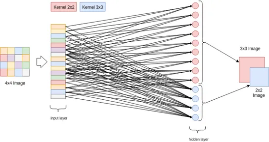
Figure 1.2: Convolutional layer on a 4× 4 image with 1 channel, and with a 2 × 2 and a 3 × 3 kernel with stride 1. The links show how the pixels contribute to the final convolution.

Each convolutional layer applies different kernels to compute the convolutions, and this set of kernels compose our weights. In our last example, one kernel could be of dimensions 5_{× 5 × 3, so that its} depth matches the inputs depth. In figure 1.2 we have an example of a convolutional layer, with two different kernels applied, although normally all kernels of a layer have the same dimensions. In a traditional CNN architecture there are other layers besides the convolutional layers such as fully connected layers or pooling layers.

Once obtained the weights using convolution, we could use them to classify the images, for example with a softmax classifier[KSH12], but this can be computationally challenging due to the big number of weights. A pooling layer is used to reduce dimensionality.

The two most common pooling functions are the average pooling, that computes the mean value of a region of the convolved image, and the max pooling, that computes the max value of a region of the convolved image. Figure 1.3 shows an example of a max pooling layer.

Figure 1.3: Max pooling with a 2× 2 filter and stride 2. Image retrieved from [Com16a]

Summarizing, a convolutional neural network is comprised of one or more convolutional layers with nonlinear activation functions, alternated with some pooling layers, and then followed by one or more fully connected layers as in a MLP. They are designed to take advantage of the 2D structure of an image, easy to train and have many fewer parameters than the fully connected with the same number of hidden layers, see 1.4.

Figure 1.4: Example of a CNN architecture retrieved from[Des16].

1.1.2

Object detection

Every object has its own features that make it special or different from others (for example, all circles are round). These features are used for classifying an object into one or many different categories. But what if the object is not the whole image, but in a part of it? Here is where comes localization, which finds exactly where the object is, drawing the bounding box that contains it. Finally, we find that in the image there may be not only one object but many, and we want to classify and locate all of them. The problem of finding and classifying a variable number of objects in an image is what we will call object detection1. While the field of classification is practically solved, object detection has problems and challenges that have been tackled for the past years with the use of deep learning, and different approaches have been implemented to find the balance between accuracy and speed.

1_{Some communities use the term object recognition as the problem of classifying the detected objects and define}

We can say that the problem of locating and classifying multiple objects in an image, called object de-tection, is nowadays best solved with neural networks. But before the arrival of deep learning there existed other methods to tackle this problem, the two most popular ones were the Viola-Jones frame-work[VJ01] and the Histogram Of Gradients (HOG) [DT05]. The first method is fast and simple, implemented in point-and-shoot cameras. It works by generating different simple binary classifiers using Haar features. Even though it offers real-time performance and scale/location invariance, it has a few disadvantages like intolerance to rotation, sensitivity to illumination variations, etc. The second method counts occurrences of gradient orientation in localized portions of the image (cells) and groups them into a number of orientation bins, so stronger gradients contribute more weights to their bins and effects of small random orientations due to noice are reduced. HOG is used for extracting the features of the images, and is normally paired with a Linear Support Vector Machine2 to classify them. Even though this method is superior than Viola-Jones, it is also much slower.

A few years ago, with the introduction of CNNs, researchers started developing methods for object detection using deep learning which lead to much more successful results than when using classi-cal methods. Deep learning is a class of machine learning that uses a cascade of multiple layers with nonlinear functions for feature extraction and transformation. After having introduced neu-ral networks and, particulary, CNNs in section 1.1.1, we will do an overview of the different state of the art approaches for object detection with the use of deep learning, and decide our best fit for this project. One of the first good methods developed for object detection using deep learning was Overfeat[SEZ+13], published in 2013, where they proposed a multi-scale sliding window al-gorithm using CNNs. Shortly after Overfeat, Regions of CNN features or R-CNN were introduced [GDDM13], which used a region proposal method (like selective search [UvdSGS13]) for extracting possible objects, then extracted features from each region with CNNs, and finally made the classi-fication with SVMs. Although with great results, the training had a lot of problems. That is why a year later the same author published Fast R-CNN[Gir15]. Instead of applying CNNs independently in each region proposed by selective search and classifying with SVMs, the latter applied the CNN on the complete image and then used a region of interest (RoI) pooling layer[Gir15] with a final feed-forward network for classification and regression. This approach was faster, and with the RoI pooling layer and the fully connected layers the model became end-to-end differentiable and eas-ier to train, but it still relied on selective search which was a problem when using it for inference. Shortly, You Only Look Once: Unified, Real-Time Object Detection (YOLO) paper by Joseph Redmon [RDGF15] was introduced, which proposed a simple CNN approach with great results and high speed allowing, for the first time, real time object detection. Instead of applying the model to an image at multiple locations and scales, they applied a single neural network to the full image, which divides the image into regions and predicts bounding boxes and probabilities for each region. Making pre-dictions with a single network evaluation made it extremely fast, 1000x faster than R-CNN and 100x 2_{Support vector machines or SVMs[HDO}+_{98] are supervised learning models for classifying that, given the labeled}

faster than Fast R-CNN. Later on, Faster R-CNN by Shaoqing Ren was published[RHGS15], which, following on the work of[GDDM13] and [Gir15], added a Region Proposal Network (RPN) to get rid of selective search and to make the model completely trainable, from end to end. RPN ranks region boxes (anchors) and proposes the ones most likely containing objects, so that the time cost of generating region proposals is much smaller with this method than with selective search. Finally, we have two notable methods: Single Shot Detector (SSD) which takes on YOLO by using multiple sized convolutional feature maps, achieving better results and speed[LAE+15], and Region-based Fully Convolutional Networks (R-FCN)[DLHS16] which follows on R-CNN methods but replacing the fully connected layers for fully convolutional ones and building strong region-based position-sensitive classifiers, which increase speed and achieve the same accuracy as Faster R-CNN.

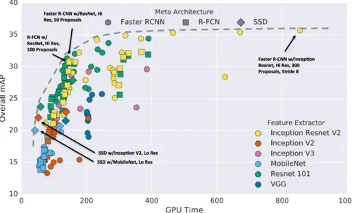
For this project we need a detector that is able to detect a person rapidly in a simple CPU, and maybe in a smartphone or tablet. Each of these object detection techniques use a base network architec-ture at the early network layers, called feaarchitec-ture extractor. These feaarchitec-ture extractors change the final behaviour of the detector in terms of speed and accuracy.

Figure 1.5 shows the performance of some of the mentioned state of the art object detectors when using different feature extractors.

Figure 1.5: Object detectors comparision trained with MS COCO dataset retrieved from[HRS+16a]

While Faster R-CNN with Inception Resnet-based architecture [RHGS15, SIV16] is top 1 in accu-racy, it implies a big loss of speed. For our purpose the best approach is using SSDs with MobileNet [HZC+_{17] or with Inception V2 [IS15], which still have a 20 mAP (mean average precision) of} ac-curacy and their GPU time is a lot less than the others.

2017 as an innovative class of efficient models created to be used in mobile and embbeded vision applications. The MobileNet architecture is based on depthwise separable convolutions, which are a form of factorized convolutions,[WLF16], that factorize a standard convolution into a depthwise convolution and a 1_{×1 convolution (pointwise convolution). In a depthwise convolution the kernels} of each filter are applied separately to each channel and the outputs are concatenated.

The MobileNet structure is built on depthwise separable convolutions, except for the first layer which is a full convolution. All layers are followed by a batchnorm[IS15] and a ReLu nonlinearity, except for the final fully connected layer which has no nonlinearity and feeds into a softmax layer for classi-fication. Figure 1.6 compares a standard convolutional layer to the factorized layer with depthwise and pointwise convolutions.

Figure 1.6: Left: a standard convolutional layer. Right: Depthwise Separable convolutions. Retrieved from [WLF16].

SSD: Single Shot Multibox Detectorpaper[LAE+15] was released at the end of November 2016 and reached new records in terms of performance and precision for object detection, scoring over 74 % mAP at 59 fps on standard datasets such as PascalVOC and COCO. The name Single Shot means that, like in YOLO, the tasks of object localization and classification are done in a single forward pass of the network, simultaneously predicting the bounding box and the class as it processes the image.

The SSD approach, shown in figure 1.7, is based on a feed-forward convolutional network that pro-duces a fixed number of bounding boxes and scores for the presence of object class instances in those boxes, finishing with a non-maximum suppression step to group together highly-overlapping boxes into a single box[HBS17, NG06]. The early network layers are based on a standard architecture used for high-quality image classification (truncated before any classification layers). In this project the base architecture is MobileNet, but in the original paper they use VGG-16. After the base archi-tecture, a set of convolutional feature layers is added, which decrease progressively in size. Instead of only using each feature map as input for the next feature layer, they reshape this feature map into a vector, making the output be the join of all these vectors. This allows predictions of detections at multiple scales, for each feature map has information in a different, each time bigger, region of the image.

Figure 1.8: Matching of default boxes with ground truth boxes retrieved from_[LAE+15_]

During training, the ground truth information needs to be assigned to specific outputs in the fixed set of detector outputs. This means that some of the default bounding boxes have to be assigned to their corresponding ground truth detection, and the network has to be trained accordingly, see 1.8. Here is where they use Multibox, by matching each ground truth box to the default box (which vary over location, aspect ratio, and scale) with the best jaccard overlap[Jac01]. Unlike Multibox, they match default boxes to any ground truth with jaccard overlap higher than a threshold, simplifying the learning problem by allowing the network to predict higher scores for multiple overlapping boxes. The SSD training objective is derived from the Multibox objective but extended to handle multiple object categories. They use Smooth L1 location loss, which measures how the network predicted bounding boxes and the ground truth ones differ, between the predicted box and the ground truth box parameters, and a softmax loss for the confidence loss, which measures the reliance of the network to have an object inside a bounding box, so that the overall objective loss function is a weighted sum of the localization loss and the confidence loss:

L(x, c, l, g) = 1

N(Lcon f(x, c) + αLl oc(x, l, g)),

where N is the number of matched default boxes, l the predicted box, g the ground truth parameters, and c the set of classes confidences.

negative training examples. This imbalance between the number of positive and negative examples is improved by using only a part of the negative examples (sorted using the highest confidence loss for each default box) so that the ratio between positive and negative examples is 3:1. Finally, to make the model more robust to various input object sizes and shapes, they randomly sample each training image, augmenting the training data. The non-maximum suppression applied at the end of the network is essential to prune the large number of boxes generated: filtering by the confidence loss and the jaccard overlap ensures that only the most likely predictions are retained by the network.

1.1.3

Object tracking

Object tracking is mainly the process of detecting an object in successive frames from a video. Track-ing multiple objects in videos is an important problem in computer vision, applied in various video analysis scenarios, such as visual surveillance, sports analysis, robot navigation and autonomous driving. We have already talked about object detection, and one may wonder where are the differ-ences between tracking and detection.

First of all, normally, tracking is faster, due to the fact that in each frame you have information about the object from the previous frames such as appearance, speed and direction. Second, tracking can handle some occlusions and preserve the identity of the object. Object detection can be a preceding step to object tracking, performed to check existence of objects in a frame and to precisely locate and classify the object.

Once the object is found, object tracking is used to follow the object through the consecutive frames. In each frame the movement of the object is computed by means of the motion model and the aspect by means of the appearance model. With the motion model we can predict a region that contains the object in the next frame, and with the appearance model we can use this region to find a more ac-curate position. As the appearance of the object can change drastically, a classifier that categorizes a region of the image as either an object or background is used. In image classification we have online and offline classifiers. Online classifiers are the ones trained at runtime, using very few examples at a time, while offline classifiers are trained using thousand of examples. The image classification used on trackers is created in an online manner, due to the fact that the results are needed at runtime.

Just like object detection, object tracking has different state of the art methodologies. While there exist different ideas studied under object tracking, such as optical flow, Kalman filter (which we will talk about in the next chapter) and meanshift and camshift, we will focus on those that can track a single object located first by an object detection algorithm. One of the first "trackers by detection", already obsolete, is the Boosting tracker [GGB06]. This tracker is based on an online version of Adaboost[FS97], the algorithm used in the Viola-Jones framework for detecting faces, trained at runtime with positive and negative examples of the object. For each frame, the classifier runs on every pixel in the neighborhood of the previous location, recording the maximum score where the location

of the object is. One of the problems of this tracker is that one does not know when the tracking has failed, as it always shows a location for the object. Another tracker is the Multiple Instance Learning (MIL) tracker[BYB09], based on the boosting tracker but instead of considering only the location of the object as a positive example when training, it looks in a neighborhood around the object and generates several positive examples. This tracker does not drift as much as the boosting tracker, and works well under partial occlusion, but still has the problem of the little reliability of the tracking failure reporting. Another tracker is the Kernelized Correlation Filters (KCF) tracker, based on[HCMB14], from the previous two trackers uses the fact that the multiple positive samples in the MIL tracker have large overlapping regions. This tracker is faster and more accurate than MIL and it reports tracking failure better, its only problem is that it does not recover from full occlusion. Now we have the Tracking, Learning and Detection (TLD) tracker from[KMM12], which, as the name says, tracks, learns and detects the object frame to frame. The detector localizes all appearances that have been observed so far and corrects the tracker, if necessary, and the learning estimates detector’s errors and updates it to avoid them in the future. TLD works very well in occlusions over multiple frames and keeps track on scale changes, but it can have a lot of false positives. Finally, in 2015 the now state of the art tracker Clustering of Static-Adaptive Correspondences for Deformable Object Tracking (CMT),[NP15], appeared. Its main idea is to break down the object of interest into tiny parts (keypoints) and in each frame try to find these keypoints. First, they track the keypoints from the previous frame to the current frame by estimating its optical flow, and then they match the keypoints by comparing their descriptors. After this, every keypoint votes for the object center, so that the keypoints in the current frame that do not match the center are removed. The new bounding box is computed based on the remaining keypoints.

1.2

Quadcopter control

In the last few years there has been a growing interest in robotics, in concrete in Unmanned Aerial Vehicles (UAV). The advances in technologies like microcomputers and aerodynamics have made possible the appearance of small, low cost and easy to manage UAVs. Navigation is more challenging in flying robots than in ground robots, due to the fact that they require feedback to stabilize. For this reason, interest in tracking objects is increased when it is made with a flying robot. In particular, our focus will be on a small Vertical take-off and landing UAV, the quadcopter. Quadcopters have low dimensionality, good maneuverability, payload capability, and also a high energy consumption. Our need is for a low cost, easy to manage, that can be programmed quadcopter, and for this we chose the AR.Drone 2.0.

1.2.1

AR.Drone 2.0

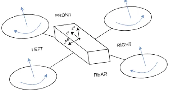
A quadcopter is a multirotor helicopter with four actuators (propellers), each providing a force in the body-fixed z-direction and a torque to the body. The AR.Drone 2.0 is a quadcopter in x-configuration,

which means that the rotors are not aligned on the principal axes of the body-fixed coordinate-system, as in the+-configuration, see 1.9.

Figure 1.9: Quadcopter with x-configuration representation, with body-fixed coordinates frame B

Movements are obtained by changing the pitch, yaw and roll angles, and by changing the vertical speed, 1.10. To hover, all rotors may speed at the same velocity such that the global force of the quadcopter cancels the gravity force. For moving forward (backward) both front (rear) rotors have to decrease their velocity while the rear (front) ones increase them. The same applies for left/right moves and rotors.

Figure 1.10: Roll, pitch, yaw and throttle movements

All quadrotors have two coordinate frames: the inertial frame (earth-fixed frame) and the base frame (body-fixed frame). This implies a system of six degrees of freedom (x, y, z, pitch, roll, yaw), con-trolled by adjusting the rotational speeds of the four rotors. With this, our system has four inputs

and six outputs, so some assumptions are made in order to control it: pretending the quadcopter to be a rigid body and the structure to be symmetric (no ground effect).

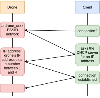
Without entering in depth in the explanation of the AR.Drone’s hardware we will talk about the main sensors and actuators in the drone and how does its communication work. The engines have three current phases controlled by a micro-controller that makes sure all the engines work in coordination and stop if any obstacle is found. The drone uses 1000 mAh, 11.1V LiPo batteries to fly, and lands when it detects a low battery voltage. It has many motion sensors, located below the central hull: an inertial measurement unit, used for automatic pitch, roll and yaw stabilization and tilting control; an ultrasound telemeter, for automatic altitude stabilization and assisted vertical speed control; a camera aiming towards the ground, for automatic hovering and trimming; a 3-axis magnetometer and a pressure sensor. Finally, the AR.Drone 2.0 has a frontal camera, a CMOS sensor with a 90 degrees angle lens, that provides 360p or 720p image resolutions (also used for the ground camera), with a frame rate between 15Hz and 30Hz. The connection with the drone is made via a WiFi network:

Figure 1.11: AR.Drone 2.0 Wifi connection

Once the connection is established we have 4 main services for communication:

• The control and configuration of the drone is done by sending AT commands on UDP port 5556. These commands are to be sent on a regular basis (30 times per second).

• Information about the drone (status, position, speed, etc.) - navdata - is sent on UDP port 5554.

• A fourth communication channel (control port) can be established on TCP port 5559 to transfer critical data.

1.2.2

Available open-source libraries

Any client device supporting WiFi can control the AR.Drone 2.0. But what are the commands that the drone understands? And how can we make it fly?

Parrot created a documentation[PBED12] that explains the format of the text strings that can be sent to the drone to control its actions (AT commands). According to this documentation: These

strings are encoded as 8-bit ASCII characters with a Carriage Return character as a new line delimiter. One command consists in the three characters AT* followed by a command name, an equal sign, a sequence number, and optionally a list of comma separated arguments. An AT command must reside in a single UDP packet, and the maximum length of the total command can’t exceed 1024 characters.

With this documentation and these AT commands, we could be able to create our own framework for controlling the drone, but that would take time, and in this project our main objective is not to create a framework to control the drone, but to be able to make the drone follow a person. There exist open-source libraries that can ease our work:

• Parrot also created an SDK that simplifies the work of writing an application to remotely control the drone. This SDK is divided into two libraries: ARDroneLIB and ARDroneTool. With these two libraries the work of controlling the drone is much more easier. But it is still hard to understand, the documentation is outdated and the few examples on Linux only work on 32-bit computers.

• Another famously used library for controlling the AR.Drone 2.0 is ardrone_autonomy, a ROS driver based on the Parrot SDK. ROS (Robot Operating System) is a set of utilities and libraries for implementing all different kinds of functionality on robots. The problem of using ROS is that some time is needed to get familiar with its structure.

• If you are familiar with node.js the node-ar-drone is your module. NodeJS is a popular plugin-based JavaScript server platform, which runs locally.

• For Python we have several open-source libraries, but they have basically the same format: a python document where several functions that create AT commands sent to the quadcopter are written, and with some low-level functions that manage the navdata received from the quad-copter. PS-Drone is one of these libraries, it is designed to also run on really slow computers, has a blog where bugs or question can be asked and are pretty quickly answered, and there exists a documentation with all the functions explained and some easy examples shown.

In the previous chapter we discussed the different available techniques that can be used for the pur-pose of controlling a quadcopter by following a person with the use of computer vision, in particular object detection and object tracking, and introduced the AR.Drone 2.0 hardware specifications to-gether with a series of open-source libraries created for the quadcopter’s easy control. In this chapter we use the object detection and tracking methods from sections 1.1.2 and 1.1.3 to create a software able to keep track of a person through the quadcopter’s movement, recover from tracking failure, and move the quadcopter accordingly to the person’s movements, with the use of one of the open-source libraries introduced in 1.2.2 to easily send the commands to the drone.

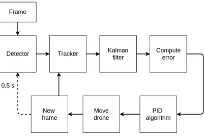
In figure 2.1 a flux diagram of our implementation is shown, with the introduction of some new elements of which we will talk about in the next sections, like the Kalman filter or the PID algorithm.

Figure 2.1: Schematic representation of the software structure.

The AR.Drone 2.0 sends every few milliseconds a frame captured from its camera to our device, and with the processing of each of these frames we will be able to send the commands to the drone that will make it go to a certain position. To simplify, we fix this position to be, in each frame:

• x so that the person’s bounding box horizontal center corresponds to the horizontal center of our frame.

• y so that the person’s bounding box vertical center corresponds to the vertical center of our frame.

• z so that the person’s bounding box height is close to the person’s bounding box height at the starting frame.

With these requirements a quadcopter controller is created, to find the best combination between the drone’s stability and movement.

In the next sections we will thoroughly explain the different approaches used in each step of the implementation.

2.1

Detection and tracking of the person

Once the drone takes off, and after a few seconds to let it stabilize, the processing of the frame starts and an object detector is used to find persons in the image. As no interaction with the program is needed, it is required that only the person to be followed stands in front of the drone, otherwise it could detect another person to track. The object detector used is based on the SSD approach and has as feature extractor the MobileNet architecture[LAE+15, HZC+17]. This approach was chosen for its high speed (it can be computed in a smartphone CPU), and its great accuracy given the cir-cumstances.

The object detector is used to find the person in the first frames. Once detected, the corresponding bounding box is used to keep the detection through the following frames with an object tracker. In section 1.1.3 we explained several object trackers and introduced the state of the art: CMT[NP15], but the software used in the detection, explained in 3.2.2, forces us to use the OpenCV implemen-tation of KCF[HCMB14]. This tracker is able to obtain the x and y center positions of our person in the frame. This is, in each frame the initial bounding box is moved through the image to wrap around the person. But this bounding box does not change in area, it always has the same width and height, which makes impossible to know the distance between the drone and the person by only using the tracker. To solve this, a combination between our detector and our tracker has been devel-oped in this project, to try to find the best balance between speed and the accuracy of the person’s bounding box. In figure 2.2 we observe a schematic representation of how this balance is obtained. The distance between the quadcopter and the person is updated every half second, also preventing the tracker from drifting, by using the object detector with only a part of the image that contains the person. With each of these new detections a new tracker is created, initializing it with the bounding box obtained by the detector.

2.2

Kalman filter and error computation

The AR.Drone 2.0 is not the best quadcopter in the market, and when flying or hovering there exists a trembling in the quadcopter that entails a trembling in the frames. Also, the tracker used does not produce a fluid trajectory of the detected bounding box between frames. This noise can be reduced with the help of the Kalman filter. The Kalman filter is an algorithm that uses a series of observations over time and a predictive model, considering that none of them are perfect, and tries to find the best balance between them, creating a detection that is more accurate that with only using each observation alone.

Next we will explain the setup from which we will create our Kalman filter:

Let x_kbe the state vector that describes our person’s position and velocity at detection k

x_k=         x_k yk ˙ xk ˙ y_k        

where(x, y) is the position in pixels of the person in the frame, and (˙x, ˙y) is the velocity (the deriva-tive of position with respect to time).

We assume now that between the detections k_{− 1 and k there is a constant stochastic} accelera-tion a_k = [ak_x, ak_y] normally distributed with mean 0 and standard deviation σa. We know, from

kinematics, that with initial state[x₀, y₀, ˙x0, ˙y0], we have:    ˙ x(t) = ˙x₀+ a_xt ˙ y(t) = ˙y0+ ayt so that    x(t) = x0+ ˙x0t+ 12axt2 y(t) = y0+ ˙y0t+12ayt2 .

From this, we observe that our state in detection k is              x_k= x_k−1+ ˙x_k−1∆t_k+1₂ak_x∆t2 y_k= y_k−1+ ˙y_k−1∆t_k+1₂ak_y∆t2 ˙ x_k= ˙x_k−1+ ak_x∆t_k ˙ yk= ˙yk−1+ aky∆tk

which concludes that

        xk yk ˙ x_k ˙ y_k         =         1 0 ∆t_k 0 0 1 0 ∆t_k 0 0 1 0 0 0 0 1                 xk−1 yk−1 ˙ x_k−1 ˙ y_k−1         +         1 2∆t 2 k 0 0 1₂∆t2_k ∆tk 0 0 ∆t_k           ak_x ak_y  

that can be expressed as

x_k= F_kx_k−1+ G_ka_k with F_k=         1 0 ∆t_k 0 0 1 0 ∆t_k 0 0 1 0 0 0 0 1         , G_k=         1 2∆t 2 k 0 0 1₂∆t2_k ∆tk 0 0 ∆t_k         .

Setting w_k= G_ka_kand knowing that a_kis a stochastic variable we can assume that w_{k∼ N (0, Qk}) is the zero mean Gaussian distributed process noise, with Q_kbeing the covariance matrix from time

step k_{− 1 to time step k:} Q_k= G_kGT_kσ_a2=         1 4∆t4kσ 2 ax 0 1 2∆tk3σ 2 ax 0 0 1₄∆t_k4σ2_a y 0 1 2∆t3kσ 2 ay 1 2∆t3kσ 2 ax 0 ∆tkσ 2 ax 0 0 1₂∆t_k3σ2_a y 0 ∆tkσ 2 ay         The observations

At each time step k a noisy measurement z_kof the true position of the person is made. Let us suppose this noise v_k is also normally distributed with mean 0 and standard deviationσ_z= [σ_z

x σzy]:

z_k= H_kx_k+ v_k

As our observation is of the person’s position, and not its velocity, we have that H_k= [1 1 0 0] and the covariance matrix of the observation is

R_k=   σ2 zx 0 0 σ2_z y  ,

for all time steps k.

Initial state

The filter is not initialized until an observation is made. The initial state is composed by the first observation for the position and[0, 0] for the velocity. As this initial state is not know perfectly, we set as initial covariance matrix

P=         σ2 x 0 0 0 0 σ2_y 0 0 0 0 σ2_˙x 0 0 0 0 σ2_˙y         .

After preparing the settings needed to create the filter, we can explain how does it work and how is the previous setup used for the computation of an estimated position.

The Kalman filter is a recursive estimator, which means that only the estimated state from the pre-vious time step and the current measurement are needed to compute the estimate for the current state. At every time step the algorithm has two stages:

• The Predict step. Uses the estimated state from the previous time step to produce an estimate at the current time step. This predicted state is also know as the a priori state estimate because no measurement information has been incorporated in the estimation.

• The Update step. The current a priori prediction is combined with the current observation to refine the state estimate. The updated step is also known as the a posteriori state estimate.

The state of the filter is represented by two variables: the ˆx_m|nis the state estimate at time step m given n≤ m measurements, and the Pm|n is the error covariance matrix at state estimate ˆxm|n. The equations of the Kalman filter for the predicted step are

ˆ

x_k|k−1= F_kˆx_k−1|k−1 (2.1)

P_k|k−1= F_kP_k−1|k−1F_kT+ Q_k (2.2)

and for the updated step are

S_k= R_k+ H_kP_k|k−1HT_k (2.3)

K_k= P_k|k−1HT_kS−1_k (2.4)

ˆ

x_k|k= ˆx_k|k−1+ K_k(z_{k− Hk}ˆx_k|k−1) (2.5)

P_k|k = (I − K_kH_k)P_k|k−1(I − K_kH_k)T+ K_kR_kK_kT (2.6) where S_k is the innovation covariance, K_kthe Optimal Kalman gain, ˆx_k|k the a posteriori state esti-mate, and P_k|k the a posteriori state estimate covariance.

At each iteration the tracker updates the position of the person, and this position is improved by using these equations of the Kalman filter. The filtered position returned by the Kalman filter is the

a posterioristate estimate computed in (2.5).

As we explained in the introduction of this chapter, the quadcopter’s 3D desired position depends on the bounding box created by the tracker. With the Kalman filter, the(x, y) center point of the bounding box has been improved, but our objective is to minimize the difference between the center of the AR.Drone captured frame and this filtered position. Moreover, the quadcopter distance from the person has to be computed and controlled, we have to obtain the distance between the person and the quadcopter at startup and try to maintain this same distance during all the iterations. For this reason, we use the height of the bounding box at the first detection and compare it with the actual height. These differences compose an error that we will try to minimize by sending the correct commands to the drone. This 3-dimensional error is

       e_x = f_x −wf 2 e_y = hf 2 − fy e_z= h_k− h0

where f_x, f_y is the filtered position, w_f, h_f is the resolution of the quadcopter’s front camera, h0 is the height of the person’s bounding box at the first detection and h_k is the height of the person’s bounding box at the actual iteration.

Knowing that in the roll movement the quadcopter goes right when the e_x error is positive, to go right the horizontal center of the frame has to be smaller than the x coordinate of the observation, and to go left it has to be bigger. However, OpenCV reads images vertical axis from top to bottom,

for this reason, and knowing that the throttle movements goes up when the e_y error is positive, the quadcopter goes up when the vertical center of the frame is bigger than the y coordinate of the observation, and goes down when it is smaller.

2.3

PID controller

Once the position of the person is obtained, its noise is removed with the Kalman filter and the er-ror between person and quadcopter is computed, we can move the quadcopter to correct this erer-ror. But to do this we need a controller that helps us create a fluid trajectory, to avoid changes in the orientation at every frame. In this section we will explain the controller used, called Proportional-Integral-Derivative or PID controller.

The PID controller is the most common control algorithm used in the industry of automation. It is a control loop feedback mechanism which computes the deviation between a given value (measured process value) and a desired value (set point) and corrects it based on the proportional, derivative and integral terms (giving the controller its name). In figure 2.3 we have a block diagram that shows how a PID works.

Figure 2.3: PID algorithm_[Com16b].

The r(t) value represents the set point and the y(t) value the measured process value. The u(t) value is the control signal and is described by the sum of the three terms: the P-term (proportional to the error), the I-term (proportional to the integral of the error), and the D-term (proportional to the derivative of the error). The equation of the PID controller is described by:

u(t) = K_pe(t) + K_i

Z t 0

e(t)d t + K_dd e(t)

d t (2.7)

The controller has to be tuned in order to suit the dynamics of the process to be controlled. Giving the controller the wrong K_p, K_iand K_dparameters will lead to instability and slow control performances. There exist different types of tuning methods that can be used:

• Trial and Error method. With this simple method first we have to start with both Kiand Kd

parameters to zero and increase K_p until the system reaches an oscillating behaviour. Then, we adjust the K_i parameter to stop the oscillation and finally adjut K_d for faster response. • Process reaction curve technique. This method produces response when a step input is

applied to the system. At first we apply some control output to reach a steady state (close one), then, in open loop, we generate a small disturbance and the reaction of the process value is recorded. This process curve is then used to calculate the K0sparameters. The method is performed in open loop so no control action occurs and the process response can be isolated. • Zeigler-Nichols method [ZN93]. In this method, as in trial and error, the Ki and Kd

param-eters start at zero. The proportional gain is increased until reached the ultimate gain, K_u, at which the output of the loop starts to oscillate. The term K_u and the oscillation period T_u are used to set the gains as showed in figure 2.4.

Figure 2.4: Table showing the Ziegler-Nichols method

But to tune a quadcopter, and without entering into more complicated algorithms, the best of these tuning methods is Trial and Error. Also, although for other systems the integral term is adjusted before the derivative one, in quadcopters is best to tune first the derivative one, and the integral has to be very small to avoid oscillations.

2.4

Drone movement

As explained in section 1.2.1, the AR.Drone 2.0 has four movements: roll, pitch, yaw and throttle. To control the quadcopter, a PID controller has to be created for each of these movements. Because of this, in this project we will have four controllers, each of which has to be tuned independently to find the correct parameters that will led to a smooth movement in its direction. The roll movement is modified by looking at the x-error filtered with the Kalman filter. After being computed, this error is then passed to the x-PID controller, which returns the velocity that has to be passed to the quad-copter. Equally, the throttle movement is modified by looking at the y-error filtered with the Kalman filter and then computing its velocity with the y-PID controller. For the pitch movement the velocities are obtained with the z component, when comparing, every half second, the difference between the original height of the person and the actual height. Finally, we have the yaw movement, that we did not implement for this project.

In section 1.2.2 we introduced different ways of sending to the quadcopter the commands needed to produce these movements. Although a few of them are valid to meet with our objectives, we chose the one that uses Python as programming language: the PS-Drone API. In the next chapter we will explain how this library is structured and how the commands are sent to the quadcopter.

In this chapter we will explain how the theoretical framework from the previous chapter has been implemented.

3.1

Source code organization

The software created for this project is written in Python 2.7 and uses OpenCV 3.4.0 to obtain the pre-trained model for the detection. The computer used is a Dell XPS 13 with an Intel(R) Core(TM) i7-7560U CPU @ 2.40GHz. All the computations, including the detection of the person with a neural network, are made in this computer. All the source code can be found in the Github repository1

Figure 3.1 shows the project’s class diagram with the structure of the system.

Figure 3.1: Class diagram of the implemenation.

The program is composed of the following files:

• main.py The main file initializes the quadcopter with the PS-Drone API, and creates a frame grabber that is passed to the tracker. The PID parameters are initialized here and the network used for the detection is extracted from a file in the containing folder.

• tracker.py This is the most important file of the program. For every frame, the detector and the tracker work together to keep the bounding box of the person, then the Kalman filter obtains an improved position and the controller moves the drone. Finally, the parameters for the next iteration are updated.

• kalman_filter.py Implements the equations explained in section 2.2.

• pid.py This file contains a class to modify and set the parameters of the pid controller. • ps_drone.py This is an external file and contains the PS-Drone API retrieved from

www.playsheep.de/drone.

• move_drone.py This file contains all the necessary commands to move the drone. It also con-tains functionalities to change the desired velocities that will be used by the PID controller.

3.2

Software explanation in depth

In this section we will explain how the classes from figure 3.1 are implemented.

3.2.1

Initialization

In figure 3.2 we have a flux diagram of the drone startup. Once the program is started, the first thing to do is check whether the quadcopter has enough battery to take off or not. With low battery the AR.Drone 2.0 can show video images but does not take off.

3.2.2

Tracking algorithm

Figure 3.3: Flux diagram of the tracking implemenation.

In figure 3.3 we have a flux diagram showing how the tracking algorithm is used in the software, after the startup of the system (showed in diagram 3.2), and followed by the correction of the position with the Kalman filter and the move of the quadcopter using the PID controller. The tracking keeps in

the loop until the user stops the quadcopter by clicking the Esc keyboard button, which automatically makes the drone land.

Detection and tracking configuration

As explained in section 2.1, both detector 1.1.2 and tracker 1.1.3 are combined to obtain a robust tracking of the person. The detector is created using the dnn module of the OpenCV library. In paticular, a Caffe[JSD+14] pre-trained model is used to create the object detector, which is a version of the original Tensorflow implementation from[AAB+16]. This pre-trained model allows us to use an implementation of the MobileNet-SSD network, trained with datasets such as COCO and PASCAL VOC, without wasting time doing it ourselves, and obtaining a model that detects 20 objects in images (dogs, cats, people, sofas, etc.). To use a pre-trained Caffe model with the dnn module of OpenCV we need two files that can be retrieved from the Caffe website:

• A Caffe prototxt file that defines the structure of the neural network. • A binary .caffemodel file that includes the pre-trained model.

Now that we understand how the network is created and used to detect the person at each frame, let’s explain how the tracker works. OpenCV 3.0 comes with a tracking API with 6 different trackers, some of which were explained in 1.1.3. Our choice was the KCF tracker which has the best accuracy, although it does not recover from full occlusion. The tracker is initialized using the bounding box retrieved from the detector and it is updated with every frame.

But, as explained in section 2.1, the tracker update does not change the dimensions of the bounding box, so the distance from the quadcopter to the person cannot be computed with only this solution. That is why we created a combination between detection and tracking showed in figure 2.2 , which finds a balance between speed and accuracy.

Filtering the position

In section 2.2 we explained in depth the equations used to create the Kalman filter for this partic-ular case. Basically, we assumed a constant velocity model with an acceleration of the pixel with a diagonal covariance. The Kalman filter class is initialized with 8 parameters:

• ax, ay: The standard deviation of the pixel acceleration (x,y respectively).

• rx, ry: The standard deviation of the pixel position observation (x,y respectively). • px0, py0: The standard deviation of the pixel initial position (x,y respectively). • pv0, pu0: The standard deviation of the pixel initial velocity (x,y respectively).

The initial state vector x_0|0(position and velocity) is assumed to be zero, and with the(px0, p y0,

pv0, pu0) parameters the initial state covariance matrix P0|0can be created.

At each iteration k the Kalman algorithm follows the steps observed in the diagram from figure 3.4 which is based on the equations and matrices explained in section 2.2. The new observation and the time of the observation are passed to the filter. Using the difference between the time of the last observation and this observation time, the F, H, Q, R matrices are computed. Then, the linear model prediction is fused with the observation using the Predict-Update steps, and the new state is returned.

Figure 3.4: Flux diagram of the Kalman filter

PS-Drone

Before talking about the PID controller and how the velocities are computed, let’s first explain how the used library works, and which parameters it needs in order to send the correct commands to the quadcopter, that make it move as desired.

PS-Drone is created in a single file, called ps_drone.py, and has a complete documentation found in www.playsheep.de/drone. For this project we only use the functions to configure the drone, to obtain video images, and to move the drone in the desired direction. Here is the list of functions used:

• startup(): to connect to the drone. • reset(): initiates a soft reset of the drone.

• trim(): the drone sets the reference on the horizontal plane.

• getSelfRotation(): the drone measures out the yaw gyrometers self spinning.

• hdVideo(): sets the drone’s video stream to H.264 encoded, with an image resolution of 1280× 720.

• frontCam(): switchs to the drone’s front camera.

• startVideo(): activates and processes drone’s video, images are available in the VideoImage attribute.

• getBattery().

• VideoImageCount: sequential number of the decoded video images stored in VideoImage. • VideoImage: contains the actual video-image of the drone as an OpenCV2 image-type, when

video is activated.

• VideoDecodeTimeStamp: time when the video image in VideoImage was decoded. • VideoDecodeTime: time needed to decode the video image in VideoImage.

• move(): drone moves to all given directions in given speed. The usage is as follows: move(roll, pitch, throttle, yaw). This is:

– roll: a float value from -1 to 1, where -1 is full speed to the left and 1 full speed to the right. This value, called the φ-angle, is a percentage of the maximum inclination configured for the left-right tilt.

– pitch: a float value from -1 to 1, where -1 is full speed backward and 1 is full speed forward. This value, called the θ-angle, is a percentage of the maximum inclination configured for the front-back tilt.

– throttle: a float value from -1 to 1, where -1 is full speed descent and 1 is full speed ascent. This value, called gaz, is a percentage of the maximum vertical speed.

– yaw: a float value from -1 to 1, where -1 is full speed left spin and 1 is full speed right spin. This value, calledω, is a percentage of the maximum angular speed.

• stop(): the drone stops all movements and holds position. Note: Setting the move() parameters all to 0 would not stop movement, but stop the acceleration. To stop movement this function has to be used.

The startup() function creates a socket that connects to the quadcopter’s IP, which is 192.168.1.1 as default, and sends the four initial commands to the drone. Then two processes for the VideoData and the NavData (sensor data) configuration are created. These two processes send to the quadcopter the configuration data needed to initiate the communication through the video data and the navdata