ANALYZING JUDICIAL COURTS’
PERFORMANCE: INEFFICIENCY
VS. CONGESTION
*MARTA ESPASA
ALEJANDRO ESTELLER-MORÉ
University of Barcelona & Institut d’Economia de BarcelonaAscertaining the cause/s of differences in performance between units of the public administration is at least as important as quantifying the very level of individual performance. We identify two causes: inefficiency and con-gestion. Inefficiency might be due to the fact that inputs are of relatively low quality (e.g, temporary workers) and/or, for a given quality, to the fact that inputs do not have incentives to exert their maximum level of effort. Congestion arises when the number of new cases is above the number that can be solved when full efficiency is achieved. This decomposition is ap-plied to the universe of Catalonian first instance courts for the period 2005-13 applying a fixed-effect panel stochastic frontier model (Wang and Ho, 2010). In this particular case, we conclude that poor performance is not due to inefficiency on the courts’ side, but to an increase in the litigation demand, that is, to congestion, while inefficiency tends to decrease along time and is correlated with the presence of temporary judges.
Key words: civil law courts, technical efficiency, stochastic frontier analysis,
panel data.
JEL Classification: K40, C23.
A
report issued by CESifo [EEAG (2011)] states that in Spain “(…) the ad-ministration of justice is slow and inefficiently organized, inflicting high costs on the operation of firms”. (p. 143). Such an opinion is in line with the re-sults reported by other scholars [including, among others, Barro (1997) and Acemoglu et al. (2005)], who show how the poor operation of institutions,(*) We thank participants at the II Annual Conference of the “Asociación Española de Derecho y Economía” (AEDE) held in Barcelona (UPF), June 2011, and at the European Association of Law and Economics (EALE) held in Hamburg; in particular, we thank Pablo Salvador and Alois Stutzer (our re-spective discussants), Nuno Garoupa and Veronica Grembi for their comments. We are also grateful to H-J. Wang, Francisco Javier Senac (Consejo General del Poder Judicial), the magistrate Carmen Ortiz, and Josep Montefusco for their useful comments, and especially to the two anonymous referees and the Editors of this Journal for their excellent feedback. The origin of this research was a project –in which the magistrate Luis Fernando MartínezZapater also collaborated– funded by the Generalitat de Cata -lunya through the Centre d’Estudis Jurídics i Formació Especialitzada. We gratefully acknowledge this funding and, in particular, the support of Joan Xirau and Roser Bach (Generalitat de Catalunya). Jordi Orrit provided superb research assistance to update the database. The usual disclaimer applies. Finally, we gratefully acknowledge the funding of the Spanish Ministry of Economy and Competitiveness (ECO2012-37873 and ECO2012-37131), and of the government of Catalonia (2014SGR420).
including the administration of justice, can negatively affect the market economy (such as the aforementioned high costs for firms) and lead to mistrust among citi-zens, resulting in a reduction in the aggregate output of the economy [see also Ramello and Voigt (2011)]. Thus, it is essential to determine whether a judicial sys-tem is efficiently employing public resources.
The concern in the literature for the (in)efficiency of the administration of jus-tice is not new [see, e.g., North (1990)]. Nor has it been a neglected topic for the Spanish case, where Pastor (2003a and 2003b, among many other references by this author) has repeatedly warned of the dangers of inefficiency, and proposed organi-zational reforms. Pedraja and Salinas’ (1996) empirical analysis represented a step further in this research and more recently Rosales-López (2008) and García-Rubio and Rosales-López (2010) have attempted to quantify the inefficiency of the system. Following this line of research, the aim of this paper is twofold. First, we analyse the level of inefficiency of Catalonian first instance courts and identify its explana-tory factors. Second, even if efficiency is high, courts might perform poorly as long as they are congested. Our empirical approach allows distinguishing congestion from inefficiency when assessing performance. In particular, with respect to the first aim, we carry out a stochastic frontier analysis and take advantage of panel data that –as we argue later– should permit us to improve previous findings. Specifically, we use the technique recently developed by Wang and Ho (2010).
Our results do not show a very wide dispersion in the levels of efficiency. In other words, the courts of justice –our analysis focuses on civil courts of first instance1–
tend to perform equally well, where “equally well” means with respect to the best performance measured from real practices. For users of the justice system, the fact that the ratios of efficiency are relatively high (an average for the whole period of 97.82%) might be small consolation. This is a common restriction for any analysis of relative efficiency. Yet, the positive aspect is the largely uniform performance of the administration of justice throughout the courts2, which would seem to point to
certain guarantees of equality of treatment. Moreover, and perhaps most importantly, in contrast with previous analyses we are able to show, thanks to the use of panel data, first, that efficiency –on average– tends to increase over time; and, second, that dis-persion falls over time. These two findings should also represent additional conso-lation for current and future users of the justice system.
Aside from the simple passage of time, the number of days in which temporary judges are employed tends to have a negative impact on the courts’ efficiency, while vacancies have no impact. In other words, while temporary workers hired to boost staffing levels increase the number of resolutions passed [Rosales-López (2008)], they are significantly less efficient compared with regular employees3. The application of
(1) We limit our analysis to first instance courts which exclusively deal with civil cases, and so ex-clude from the sample those first instance and instruction courts that also deal with criminal cases to ensure uniformity and consistency of the sample.
(2) As we discuss in section 1.4, our sample comprises all the civil courts of first instance in Catalonia and so our assessment of uniformity is restricted to the situation in that region.
(3) Recall productivity is accounted for by a combination of factors: economies of scale, operating efficiency, environmental factors, and production technology [see, for example, Fried et al. (2008),
a stochastic frontier analysis –in contrast with non-parametric techniques such as Data Envelopment Analysis (DEA)– allows us to estimate consistently the impact of this internal variable and of the passage of time on differences in efficiency.
The empirical literature to date –the studies examining the situation in Spain cited above aside– has looked at different countries and jurisdictional areas: Kittelsen and Førsund (1992) examined Norway and its district courts (107 decision units (DUs)); Tulkens (1993) analyzed Belgium and its Justices of the Peace (187 DUs); Schneider (2005) studied Germany and its Labor Courts of Appeal (9 DUs); Yeung and Azevedo (2011) examined Brazil and its first- and second-degree courts (27 DUs); and Deyneli (2012), for a set of European countries, apparently looked at all courts involved in civil, administrative and criminal cases (22 DUs). As mentioned above, all these studies em-ploy non-parametric techniques (specifically, DEA, except Tulkens, who emem-ploys “Free Disposal Hull” (FDH)), and use either cross-sectional data [Deyneli (2012) and Yeung and Azevedo (2011)], repeated cross-sectional data [Tulkens (1993)] or a pool of cross sections [Kittelsen and Førsund (1992) and Schneider (2005)]4. Hence, to the best of
our knowledge, this study is the first to employ a parametric technique, which as we have stressed above is particularly suited to the consistent estimation of inefficiency effects5, and uses a panel of data6. Most important, given that the efficiency analysis
pp. 7-8)]. Here, we focus solely on operating or production efficiency and –as we argue in due course– environmental factors (including a proxy for quality of resolved cases), which can be considered the most significant. In our case, the scale of production is similar between the units, while production technology is equally available to all the courts. In the empirical literature on efficiency, operating ef-ficiency is usually labeled as the net efef-ficiency of environmental factors [see, e.g., Coelli et al. (1999)]. If the factors were not filtered out (by means of being included in the frontier as control variables), the resulting efficiency would have to be labeled as gross efficiency.
(4) Note, though, that the use of non-parametric techniques is compatible with exploiting the panel nature of the data [see, for example, Tulkens and van den Eeckaut (1995)].
(5) The parametric methodology we employ is not necessarily superior to the non-parametric. In fact, each has its own advantages/disadvantages, and so the eventual choice depends on the researcher’s objective. In contrast to the parametric approach (from now on, we focus our comments on the Sto-chastic Frontier Analysis (SFA)), the non-parametric methodology has the advantage of not needing to specify a particular production function, but it does not allow for shocks in production (i.e., all de-viations from best practice are considered as inefficiency, and so efficiency scores will be biased as long as there is noise in the estimation). In addition, while the SFA requires that an error distribution be imposed (gamma distribution, half-normal distribution, truncated-normal distribution, etc.) –al-though basic results do not tend to depend greatly on this assumption [see, for example, Kumbhakar and Lovell (2000), p. 90]– this is simply unknown in the non-parametric approach, which in any case can be addressed using bootstrapping techniques [see Simar and Wilson (2007)]. In fact, in the case of the so-called “second-stage”, where inefficiency is explained through exogenous factors, unless a bootstrapping technique is applied in the non-parametric approach, Simar and Wilson conclude that “in terms of coverage of estimated confidence intervals, tobit regression is catastrophic in our Monte Carlo experiments” (p. 57). By contrast, this is not an issue in the SFA, given that we impose ex-ante a distribution function for the error term. Since our primary interest here lies in estimating the de-terminants of inefficiency, we have chosen the SFA as our empirical technique.
(6) As Kumbhakar and Lovell (2000) write, “cross-sectional data provide a snapshot of producers and their efficiency. Panel data provide more reliable evidence on their performance, because they en-able us to track the performance of each producer through a sequence of time periods”. (p. 64). Thus, using panel data will be useful in our particular case to control for personnel (as we make clear in sec-tion 1.2), but in general the approach provides a more robust efficiency analysis, avoiding the potential volatility of the results.
permits us obtaining the number of cases that in absence of inefficiency a court should annually solve, in contrast with previous analyses we are able to infer to what extent poor performance is due to inefficiency and/or to congestion.
If poor performance is due to inefficiency, new public management practices should be introduced; in the latter, the design of policies should also depend on a pre-vious assessment of the level of litigation7. Then, if litigation is socially valuable,
congestion would require an increase in the means at disposal of the justice admin-istration (basically, staff). Furthermore, note this analysis could be applied to any other public service (healthcare, university education, security, and others) as long as the output and inputs were identifiable and measurable.
The rest of the paper is organized as follows. Next, in section 1, we present our empirical framework, including an explanation of our unit of analysis –civil courts of first instance (juzgados de primera instancia)–, the specification of the frontier and of the inefficiency effects model, and our data that spans the years 2005 to 2013. The results of our analysis are presented in section 2. Section 3 concludes. 1. EMPIRICAL FRAMEWORK
1.1. The unit of analysis: the case of the “juzgados de primera instancia” In 2008, concern about the performance of the courts in Spain led the General Council of Judges (Consejo General del Poder Judicial (CGPJ)) to introduce a pro-gram aimed at modernizing the Administration of Justice (Plan de modernización de
la justicia). Among other measures it proposed implementing new technologies,
im-proving the legislation8and establishing a new judicial office (Nueva oficina judicial).
The idea underpinning this last measure was to share administrative cases between the courts regardless of the particular legal area in which each operated. As García-Rubio and Rosales-López (2010) point out a further aim of the program was to im-prove the analysis of the courts’ performance, which is precisely what we seek to do here by focusing on the civil courts of first instance (juzgados de primera instancia). Civil courts of first instance comprise a judge and a qualified court secretary (secretario judicial). Thus, all courts are unipersonal, as just one judge is empow-ered to resolve the cases with the aid of his or her court secretary. In addition, and here there is some variation between courts albeit not over time, the courts employ other staff (gestión procesal (GP), auxilio judicial (AJ) and tramitación procesal (TP)) of lower professional standing than that of the judge and court secretary9. These
(7) See, for example, Vereeck and Mühl (2000) who –based on the work of Gravelle (1990)– ana-lyze policy prescriptions on the “demand side” to reduce congestion and, hence, improve the per-formance of the administration of justice; or Esteller-Moré (2002) for a theoretical analysis of the im-position of a user charge to act as a disincentive to filing frivolous suits.
(8) See, for example, Di Vita (2010) on the effects of the complexity of legislation on the performance of the courts of justice.
(9) The main difference among each staff group is their level of academic background (from high-est, diploma, for GP till just compulsory secondary education for AJ) and labor responsibility (for ex-ample, those in GP can sign some official documents). In general, they all offer broad support to the judicial activity (communication of notifications, execute foreclosures, and so on).
courts are authorized to resolve civil disputes, i.e. lawsuits between private indi-viduals, which might include eviction orders, outstanding mortgage payments, com-mon complaints between neighbors, etc.
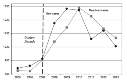
In Figure 1, we show the average evolution of both resolved cases vs. new cases for all the Catalan courts between 2005 and 2013. Until 2007, Spain enjoyed its Golden Age, an exceptional macroeconomic period. The crisis however increased the caseload in the civil courts of first instance till a peak in 2009. While in 2005 there was an average of 873.2 new cases per court, in 2009 this figure had risen to 1,311.9, i.e., a 50% increase. However, in the same period the number of cases re-solved per court increased from 855.92 to just 1,173.88, i.e., a 37% increase. Thus, while the raw data seem to confirm the conclusions of the EEAG report (2011) quoted before, it is also true that the number of resolved cases has followed the in-creasing path of new cases. In particular, since 2010, the number of resolved cases has been above the number of new cases. Thus, it seems courts have responded to an increasing workload (congestion) increasing efficiency.
Figure 1: EVOLUTION IN THE NUMBER OF NEW AND RESOLVED CASES(2005-2013)
Source: Consejo General del Poder Judicial (CGPJ), several years.
The ratio between Resolved cases (R) and New (N) cases –which is implicit to Figure 1 and referred to by the CGPJ as the “resolution ratio” (Rr)– is usually em-ployed to assess the relative performance of the courts. However, note that this ra-tio can be decomposed in the following way:
[1] Rr R R R N R N * * ≡ × =
Yet, assessing the performance from ratio [1] might offer a biased –or, at least, incomplete– picture of the performance of the courts of justice. The first factor of the ratio picks up the inefficiency component, R/R*, which tends to decrease the value of the resolution ratio if the number of resolved cases is below that of a given benchmark, which we label as R* (R<R*). The second factor picks up the conges-tion component, R*/N; even if a court resolves the optimal number of cases per year (R = R*), the resolution ratio might still be low if the number of new cases is suffi-ciently high, that is, if R*<N. Only in this latter case should we strictly speak of con-gestion. Ideally, in the absence of congestion (R* = N), Rr would be a good perfor-mance measure. However, this is not necessarily the case. All in all, according to the above decomposition, we should be able to identify to what extent the value of the resolution rate is due to the inefficiency attributable to the courts side and to a prob-lem of congestion. Next, we specify the empirical model that allows us to answer this and other related questions10.
1.2. Model specification: the frontier
In order to estimate judicial inefficiency, first, we have to estimate the best prac-tice (this idea dates back to 1951, and was proposed by Koopmans), that is, the sto-chastic frontier of production of the civil courts of first instance. Thus we define the following equation:
(10) Our (in)efficiency analysis specifically enables us to endogenously estimate this benchmark. (11) Resolved cases is a heterogeneous measure of court activity, as it includes both asuntos resueltos and ejecutorias, where the latter are a consequence of the former (basically, involving procedures im-plementing judges’ decisions), and so the amount of effort required for ejecutorias should be lower. We have distinguished between both types of case, and our results do not change qualitatively. Re-sults are available upon request from the authors.
(12) This is in contrast, though, with the approach followed by Pedraja-Chaparro and Salinas-Ji ménez (1996).
[2]
New Pending New Pending
ln Resolit i 1ln it 2ln it 3 ln it ln it 2 4 2 α β β β
(
)
β(
)
= + + + + New Pending ln it ln it 5 β(
)
+ × + Trend6 7Trend2 lnNewit Trend
8 β β β + + + × Pending Trend ln it 9 β
+ × ++β9Immigrationit+β10Qualityit+ηit
where Resolitis the output, defined as the total number of cases resolved by court i in
year t11, whileη
itis a composite error term, which is described more precisely in
sec-tion 2.3. All the variables are expressed in logs, and so pending key further explana-tion of the funcexplana-tional form below, the estimates can be interpreted as elasticities. The number of resolved cases should depend on physical inputs (personnel, computers, of-fices, and so on), as well as on the system’s caseload. As argued by Schneider (2005): “[…] omitting the caseload would imply that productivity is underestimated for those years in which a court is charged with a small caseload” (p. 134)12. Additionally, we
distinguish between those new cases entering the court in year t (New) from those pending at the beginning of year t (Pending). A priori, the productivity of new cases should be higher than that of pending ones if we suppose that by definition
qualita-tively the latter are more difficult to resolve [e.g., this is also the assumption made by Beenstock and Haitovsky (2004)].
As noted in section 1.1, each court of first instance comprises a judge and a court secretary, while the number of administrative staff can vary between courts but not over time. Thus, in a panel of data it is not possible to estimate the productivity of each member of staff, while in a cross-section it would only be possible to estimate the pro-ductivity of the administrative staff. However, although estimating the propro-ductivity of each production factor is not the aim of this paper, in order to obtain unbiased es-timates of the remaining parameters and, thus, to obtain a well estimated production function, we still need to control for differences in personnel between courts. In ex-pression [2] we control for this difference by means of fixed effects, αi. Note that, in common with most previous studies, by estimating a judicial production function we leave aside other physical inputs. In our case, this is due to a lack of data. Neverthe-less, in line with arguments presented elsewhere in the literature, this should not be a great problem as judicial production is very labor intensive13. Moreover, this should
be even less problematic in our case, as we are able to control for unobserved het-erogeneity. That is, we can reasonably assume that those other unobserved inputs are picked up by the fixed effects. Finally, we also include a time trend and a squared time trend in order to control for common shocks in the technology of production (e.g., in-stitutional reforms or changes in technology, such as those envisaged by the CGPJ in its Plan de Modernización, as described in section 1.1)14.
Thus, the use of panel data seems particularly convenient when controlling for common shocks and structural heterogeneity. A further source of heterogeneity between the courts could be their differing propensity to litigate depending on geographical area, although this has already been controlled for by explicitly including the number of new and pending cases in the frontier. Thus, no one court suffers discrimination in the em-pirical analysis if particular individuals under its jurisdiction tend to litigate more than average, as the court is compared with another with the same level of litigation. In spite of this control for levels, litigation might not provoke the same workload as this will ultimately depend on the nature of the lawsuits. In this sense, the effect of immigra-tion might be paradigmatic [see Calvo et al. (2004)]. Disputes involving immigrants might be more difficult to resolve as in some cases language and cultural differences might prove an additional obstacle, and the social and economic fragility of some im-migrants (primarily because of irregular place of residence) might hinder communi-cation between litigants and the justice administration. For this reason, in [2], we in-clude, in an ad hoc manner, the percentage of immigrants with respect to total population, being non-positive its expected sign, β9≤ 0. Hence, our estimates of (in)ef-ficiency are net of the potential effect of immigration (see also fn. 2).
(13) This is the approach adopted by all previous studies surveyed in the Introduction. For example, Kittelsen and Førsund (1992) argue that “while the absence of capital data is regrettable, it does not destroy the relevance of the results, since the sector is very labor-intensive” (p. 282).
(14) For ease of interpretation, but also in line with most of the previous empirical literature on the estimation of stochastic frontiers, we include a time trend and a squared time trend. However, our qual-itative results both in the frontier and in the inefficiency effects model (available upon request) remain unchanged if we employ time effects instead.
In contrast with other papers, we also try to disentangle strict inefficiency from quality15. Otherwise, ceteris paribus, it might penalize those courts passing a lower
number of resolutions, but which are of higher quality. The problem is how to mea-sure quality. We do this by dividing the number of sentences (fully or partially) non-revoked by another court with respect to the total number of court appeals. This is not a perfect measure as there is a delay between the appeal and its resolution, and so our ratio might be above one. However, we think it is the most reasonable one given the information at our disposal. We expect a negative estimate of this variable, β10≤ 0.
Dimitrova-Grajzl et al. (2011) have estimated a judicial production function like [2], but in a linear fashion. These authors tackle a potential technical problem in the es-timation of the production function, that of simultaneity bias and/or of reverse causal-ity. This would produce inconsistent and biased estimates in the frontier calling for an instrumental variables approach. In our case, though, this should not be a problem. These authors argue that on the one hand, ceteris paribus, if the number of resolved cases in a court is low, more judges may be allocated to that court. However, in the Spanish first instance courts the number of judges (uni-personal) and of the rest of staff is fixed. On the other hand, they argue that ceteris paribus, a court that is able to resolve more cases will likely see an increase in its caseload [see also Priest (1989)]. In the Spanish case, though, the lawsuit must be brought in the court located there where the defendant lives. And if there are several courts in the place of residence of the defendant, the plaintiff cannot choose, but the lawsuit is allocated to a court according to exogenous criteria, which basically aim at guaranteeing an equal caseload among courts.
Finally, note that the functional form of expression [2] is translogarithmic, i.e. we estimate a function that is as flexible as possible16. This is in contrast with
pre-vious analyses and as we will see becomes key to interpret the judicial production function. The form chosen implies that the productivity rate of new cases is not in-dependent of pending cases at the beginning of the year, which might seem reason-able since pending cases could well create something of a bottleneck. Then, from expression [2], the impact on resolved cases (in terms of elasticity, given we are work-ing with logs) of an increase in new ones is the followwork-ing:
(15) For example, Kittelsen and Førsund (1992) take it for granted (p. 278); Tulkens (1993) implic-itly recognizes that delays (or inefficiency) may be seen as a decrease in quality (p. 204, fn. 17); be-ing this latter approach also implicitly adopted by Yeung and Azevedo (2011) when they conclude that “… efficiency constitutes one aspect of overall quality” (p. 4); Ramseyer (2012) argues that due to lack of data it is impossible to gauge quality; while Christensen and Szmer (2012) leave it for future research. (16) See, for example, Coelli et al. (2005) for a definition of flexibility in this context, which is ob-viously welcome so as to provide a more precise estimation of the parameters of the model, together with other properties of the trans-log specification (pp. 211-212).
[3]
New Pending Trend
2 ln ln
R N, 1 3 5 8
ε =β + β +β +β
and similarly if we wish to estimate the impact of pending cases on the total num-ber of resolved ones. We can then test empirically whether the translogarithm is the adequate specification. Were a Cobb-Douglas specification to be preferred (common functional form employed by the previous literature) β3= β4= β5= β7= β8= β9= 0;
cases would increase by β1, independently of the initial number of new cases, pend-ing cases, and the specific moment in time. By contrast, our more flexible specifi-cation allows elasticity to be highly non-linear. Having explained the frontier, we now move to the specification of the inefficiency effects model.
1.3. Model specification: the inefficiency effects model
Up to this juncture, we have been concerned with providing a detailed expla-nation of the stochastic frontier. However, a further concern must be explaining the differences in the efficiency of the courts of first instance over time. In other words, we are interested in explaining deviations from the stochastic frontier leaving aside the error term17. In a stochastic18frontier model such as that specified in [2], we have
a composite error term:
(17) Note that given the definition of our frontier (expression [2]), our measure of technical inefficiency is outputoriented. That is, it conveys information about how many additional cases –in percen -tage terms– could be resolved while keeping demand (see fn. 6) and all staff numbers constant. (18) We refer here to a stochastic frontier production function because the output values are bounded from above by a random variable that does not only include the inputs but also the error term [see, for example, Coelli et al. (2005), pp. 243-4]. Otherwise, if the frontier were deterministic, the dis-tance to the frontier would be a mix of noise (i.e., error of estimation) and inefficiency.
(19) The factor h ensures that the model exhibits the “scaling property”. See Wang and Ho (2010) and the references cited therein for a discussion of the technical advantages of this property. In fact, according to Wang and Schmidt (2002), p.132, one of the advantages of this property is that it allows the researcher to obtain the estimates of partial effects as in any linear model. Note this linearity is immediate from [5], since the partial effect of the variables, z’s, included in hit(expression [6]) does not depend on u*.
(20) In the empirical application, we also ran a truncated normal distribution but the convergence process of the maximum likelihood function did not work.
[4]
v u
it it it
η = −
where vitis a zero-mean random error with the usual statistical properties, vit~ N(0, σv2),
and the term uitis a stochastic variable that accounts for technical inefficiency, so that:
[5] uit =h uit. i* [6] hit = f z
( )
itδ [7] ui N 0, u ,i 1,...,46,t 1,...,10 * 2 ∼ +(
σ)
= =where hitis a positive function of 1×L vector of non-stochastic inefficiency
deter-minants zit19, and δ is a vector or parameters to be estimated. The notation “+”
in-dicates that the underlying distribution is truncated from below at zero so that real-ized values of the random variable ui*are zero. We suppose ui*follows a half-normal
distribution20. Note, though, that according to [5], technical inefficiency, h
it, is a
prod-uct of a time-varying function, f(zitδ), and a time-invariant random variable (once we have accounted for structural heterogeneity in the frontier), ui*. Our purpose is
The model proposed above follows Wang and Ho (2010). Greene (2005) argues that traditional stochastic frontier models fail to distinguish structural heterogeneity in the frontier –which is critical in our case due to the equal number of judges and court secretaries in all the courts and the invariant composition of the rest of staff– from struc-tural inefficiency. In fact, by disentangling the two components we obtain the so-called “true fixed-effect model”, which basically involves controlling for fixed effects both in the stochastic frontier and in the inefficiency effects model [Greene (2005)]. Leaving aside any computational difficulties, however, such a specification gives rise to an “in-cidental parameters problem” (Neyman and Scott, 1948). That is, for a fixed T, estimates become inconsistent. In order to overcome this problem of inconsistency and yet still deal with heterogeneity in the stochastic frontier framework, Wang and Ho (2010) pro-pose a transformation of the stochastic frontier model. Specifically, after transforming the model (in our case, expression [2]) by either first-difference or within-transfor-mation (both transforwithin-transfor-mations produce the same results), the fixed effects are removed before the estimation is carried out based on a consistent maximum likelihood mator for a panel stochastic frontier model. Hence, this approach enables us to esti-mate consistently a fixed-effect stochastic frontier model by means of a within-trans-formation, and so deal with time-invariant individual heterogeneity in the frontier.
Unfortunately, though, Wang and Ho’s (2010) approach has a potential drawback. The fixed effects in the frontier might not only pick structural heterogeneity (either due to environmental factors or/and to the invariant endowment of inputs21), but also
structural inefficiency (if any). Then, if this were the case, the estimated efficiency levels would be biased, as they would be net of structural inefficiency. In our case, this should not be a great concern, as we aim at estimating the evolution of inefficiency over time and also to infer the importance of other explanatory determinants of in-efficiency different from structural ones, which are mostly unobservable.
We, then, propose the following basic specification for expression [6]:
(21) Beenstock and Haitovsky (2004) argue that the inclusion of fixed effects in the judicial production function might also pick up the fact that a court could receive harder or easier cases on average than other courts (p. 364).
[8]
hit 1%TemporaryWorkersit 2%Vacanciesit 3Trend 4Trend it
2
δ δ δ δ ω
= + + + +
where ωitis a random error with the usual statistical properties, and δiare the
para-meters to be estimated. A positive sign implies a positive contribution of the corre-sponding variable to inefficiency. In the inefficiency effects model, we also include a trending function, but in this case it aims at estimating the extent to which the level of inefficiency depends on the passing of time. Additionally, we also include an in-ternal characteristic of the courts: the percentage number of days filled by tempo-rary workers and the percentage number of days that remain unfilled or vacant. These models do not permit dealing with a potential endogeneity problem. That is why, the estimates δ1and δ2will strictly account for correlations between the importance of
each type of staff and inefficiency.
Given the previous caveat, note on the one hand, temporary workers –albeit pro-ductive– might be less efficient than regular employees, or at most, equally efficient.
This is also the hypothesis adopted by Christensen and Szmer (2012) to estimate the efficiency of U.S. courts of appeals22. In particular, these authors are able to
qual-ify – according to their respective expertise – three types of designated judges due to systematic understaffing. They find that courts with “district court judges”, who are the least expert of the designated judges, are more inefficient. Thus, they obtain δ1 > 0, but only for the least expert temporary workers, while for the rest δ1 = 0 (i.e.,
neutral impact). Unfortunately, though, we will not be able to distinguish temporary workers according to their level of expertise. On the other hand, by definition an in-creasing number of vacancies should lead to a reduction in the number of cases re-solved, and so ceteris paribus increase inefficiency. This is the result obtained by Christensen and Szmer (2012). However, δ2 could be equal to zero if the staff
mem-ber whose position is unfilled is unproductive (pessimistic view) or if the rest of the staff then tend to work harder to compensate his or her absence (optimistic view). To a certain extent, this latter hypothesis is related to the theoretical framework de-veloped by Beenstock and Haitovsky (2004). According to their model, under pres-sure (e.g., vacancies) judges – their unit of analysis – tend to exert higher efforts in order to maintain chances of promotion. Thus, this strategic reaction, which could be reasonably extended to the rest of the judicial staff, might counterbalance the neg-ative impact of vacancies such that δ2 = 0.
1.4. Data
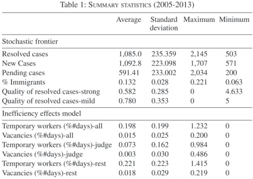
Descriptive statistics for all variables are shown below in Table 1. Our time span runs for the nine-year period, 2005-201323, and the basic units of analysis –as
pre-sented above– are the civil courts of first instance in Catalonia, including those spe-cialized in family law cases. The panel consists of 1,036 observations, with the num-ber of courts increasing over time: 110 (2005 and 2006), 112 (2007), 114 (2008) and 118 (2009-onwards) given that new courts were created during the period of analy-sis. However, in order to guarantee homogeneity, these courts were only included within the dataset two years after their creation, which explains why the number of courts varies over time24.
All the statistical information is drawn from the CGPJ (http://www.poderjudi-cial.es), with the exception of the percentage number of immigrants with respect to the overall population which was obtained from the Spanish National Institute of Sta-tistics (www.ine.es). This last variable is defined as the total number of immigrants minus those from the EU (15)25. We have defined quality before, but note we
em-(22) This work is certainly very interested, since identifies and estimates different “pathologies” of judicial inefficiency. However, we have not cited it in our Introduction, since –in contrast to those pa-pers cited therein– it does not properly estimate inefficiency, but a production function. This also ap-plies to Beenstock and Haitovsky (2004) and to Dimitrova-Grajzl et al. (2012) cited elsewhere. (23) Our sample ends in 2013, the last year available data at the moment of our analysis.
(24) We also discarded the years 2007 and 2008 for court #1 of Lleida after having detected incon-sistencies in the data for these two years.
(25) As discussed, there were 118 courts in 2009. However, they are organized geographically (par-tidos judiciales). In our sample, we have 11 areas (L’Hospitalet del Llobregat, Barcelona, Girona, Tar-ragona, Badalona, Lleida, Mataró, Terrassa, Reus, Granollers and Sabadell). Then, the percentage of immigrants was calculated for each of these broad areas, which means that each court within an area has the same percentage of immigrants.
ploy a strong version (number of fully non-revoked cases vs. number of appeals) and a mild one (including in the numerator the number of partially revoked cases as well). The percentage of temporary workers and vacancies (subscripts omitted, but cal-culated yearly for each court) was calcal-culated according to the formula:
Table 1: SUMMARY STATISTICS(2005-2013)
Average Standard Maximum Minimum deviation Stochastic frontier Resolved cases 1,085.0 235.359 2,145 503 New Cases 1,092.8 223.098 1,707 571 Pending cases 591.41 233.002 2,034 200 % Immigrants 0.132 0.028 0.221 0.063
Quality of resolved cases-strong 0.582 0.285 0 4.633
Quality of resolved cases-mild 0.780 0.353 0 5
Inefficiency effects model
Temporary workers (%#days)-all 0.198 0.199 1.232 0
Vacancies (%#days)-all 0.015 0.025 0.200 0
Temporary workers (%#days)-judge 0.073 0.162 0.984 0
Vacancies (%#days)-judge 0.003 0.030 0.486 0
Temporary workers (%#days)-rest 0.221 0.223 1.415 0
Vacancies (%#days)-rest 0.018 0.029 0.219 0
Note: Statistics based on pooled cross-sections for the whole set of courts throughout the period of analysis. Total number of observations = 1,036.
Source: Own elaboration.
[9] Temporary Wor % kers Jc Sc AJc GPc TPc 365 (1 1 #AJ #GP #TP) = + + + + × + + + +
J and S refer to judges and court secretaries, respectively, while AJ, GP and TP refer to the other staff positions. In the numerator of [9], for each staff type, we in-clude the number of days filled by temporary workers: for example, Jc is the num-ber of days filled by temporary judges. In the denominator, we include the maximum number of days that ought to be filled by regular personnel, 365. Recall from sec-tion 2.1 that in each court there is one judge and one court secretary; having said that, for example, #AJ picks up the number of AJ in the corresponding court. Similarly, in the case of vacancies we employ the following formula:
[10] Vacancie % s Jnc Snc AJnc GPnc TPnc 365 (1 1 #AJ #GP #TP) = + + + + × + + + +
While the denominator is equal to that of expression [9]26, in this case, the
nu-merator picks up the number of days unfilled for each category of personnel. Given the obvious differences in terms of the responsibilities and skills of the various cate-gories of personnel, we also calculated both indices for temporary workers and va-cancies for judges and court secretaries, on the one hand, and for the rest of the per-sonnel, on the other. If we look at Table 1, the percentage of vacancies –especially for judges and court secretaries– is very low on average. This, however, is not the case for temporary staff, where the maximum value of 0.984 for judges and court secretaries is quite outstanding. In the case of temporary workers the percentage is above 1, which means that in those cases the administration assigned reinforcement personnel. 2. EMPIRICAL RESULTS
2.1. Frontier and inefficiency effects model
Table 2 shows the empirical results. Model 1 is the basic model, where the fron-tier is specified as a Cobb-Douglas functional form, while we include a trend and control for the percentage of immigrants and for the strong version of quality. The estimate of new and pending cases is immediately interpretable as elasticity: a 10% increase in new cases results in a 5.49% increase in the cases resolved by the courts, which is above the elasticity of pending cases (2.13%). This seems reason-able as the nature of pending cases might mean it is more difficult to resolve them. Yet, given that the elasticity in both cases (and its summation) is below one, the per-formance of the courts on average generates delays. While immigration and quality have the expected negative, they are not statistically significant; the structure of staff (% of temporary workers and vacancies) do not correlate with inefficiency.
The mere passing of time, though, improves performance as is shown by the es-timates of the trend in the inefficiency effects model. Specifically, the relationship between inefficiency and time is non-linear: as long as the value of the trend is greater than 2 (note the marginal impact of the passing of time is 0.357-2 ×0.089 ×Trend)– recall in our sample: 2005 equals 1 and 2013 equals 9, the simple passing of time tends to increase performance. Thus, this represents good news for efficiency lev-els. Moreover, given the estimated non-linearity of the trend, the impact of time tends to increase over time. Yet, these results must be treated with caution as the frontier might not be properly specified. For this reason, in the models that follow we basi-cally seek to estimate more flexible production functions.
In Model 2, we estimated a translogarithmic function, and hence the interpre-tation of the estimates is not straightforward given the interactions between all the variables (see the example given by expression [3]), with the exception of immi-gration and quality that are included in an ad hoc fashion as it has only a potential influence on levels. According to a log-likelihood ratio test (λ = -2×[836.33-908.44] = 144.22, a value that is well above 11.07, the critical value at 5% for five degrees
(26) Note both expressions do not add to 1. First, as we show later, because of the use of reinforce-ment personnel; and, second, because obviously in order to sum one we still require the percentage number of days filled by regular personnel. This explains why in the regression we can include both potential explanatory variables.
T able 2: E STIMA TION O F S T O CHASTIC FR ONTIER : T O T AL NUMBER OF RESOL VED C ASES (2005-2013) (N = 1,036) Model 1 M odel 2 M odel 3 M odel 4 M odel 5 M odel 6 ln(ne w ) .549 *** 2.938 *** 2.518 *** 2.713 *** 2.905 *** 2.657 *** (18.34) (2.99) (2.55) (2.77) (2.95) (2.72) ln(ne w ) × ln(ne w ) — -.025 .008 -.009 -.021 -.006 (-.31) (.10) (-.11) (-.27) (-.07) ln(ne w ) × T rend — -.025 *** -.026 *** -.026 *** -.025 *** -.026 *** (-2.66) (-2.80) (-2.74) (-2.66) (-2.79) ln(pending) .213 *** .430 .478 .445 .441 .433 (16.16) (1.13) (1.27) (1.18) (1.16) (1.15) ln(pending) × ln(pending) — .141 *** .140 *** .139 *** .141 *** .139 *** (6.89) (6.93) (6.87) (6.90) (6.86) ln(pending) × T rend — .029 *** .029 *** .028 *** .029 *** .028 *** (6.62) (6.63) (6.57) (6.62) (6.59) ln(pending) × ln(ne w ) — -.307 *** -.312 *** -.306 *** -.309 *** -.304 *** (-5.84) (-5.98) (-5.87) (-5.88) (-5.83) T rend .001 .039 .045 .045 .038 .046 (.40) (.57) (.67) (.66) (.55) (.68) T rend 2 — -.004 *** -.004 *** -.004 *** -.004 *** -.004 *** (-3.65) (-3.76) (-3.71) (-3.63) (-3.65) % Immigrants -.133 -.588 -.575 -.603 -.591 -.608 (-.30) (-1.47) (-1.42) (-1.50) (-1.47) (-1.51) Quality of resolv ed cases-strong -.011 -.005 -.008 -.006 -.005 — (-.091) (-.45) (-.71) (-.58) (-.47) Quality of resolv ed cases- mild — — — — — -.012 (-1.28) Notes: *signif.: 10% le v el, ** signif.: 5% le v el, *** signif.: 1% le v el; C v and C u
are unconstrained constant parameters, such that C
v = ln( σv 2) and C u = ln( σu 2),
so according to the parameterization pro
v ided by Aigner et al . (1997), λ 2 = σu 2/σ v 2, if λ
= 0 there are no technical inef
ficienc
y ef
fects and all de
viations from
T able 2: E STIMA TION O F S T O CHASTIC FR ONTIER : T O T AL NUMBER OF RESOL VED C ASES (2005-2013) (N = 1,036) (continuation) Model 1 M odel 2 M odel 3 M odel 4 M odel 5 M odel 6 Inef ficienc y ef fects model T emporary w o rk ers (%#days)-all -.116 -.113 — — — — (-.62) (-.53) V acancies (%#days)-all .903 1.921 — — — — (.77) (1.18) T emporary w o rk ers (%#days)-judge — — .746 *** .567 ** — .580 ** (2.75) (2.35) (2.40) V acancies (%#days)-judge — — -0.534 -.157 — -.167 (-.45) (-0.13) (-.14) T emporary w o rk ers (%#days)-rest — — -.351 * — -.156 — (-1.82) (-.83) V
acancies (%#days)- rest
— — 1.050 — 1.659 — (.79) (1.17) T rend .357 *** .726 *** .657 *** .636 *** .716 *** .626 *** (3.66) (3.61) (4.18) (3.83) (3.72) (3.82) T rend 2 -.089 *** -.116 *** -.107 *** -.104 *** -.115 *** -.103 *** (-5.48) (-4.71) (-5.10) (-4.78) (-4.81) (-4.76) σv 2 -4.778 *** -4.913 *** -4.932 *** -4.923 *** -4.915 *** -4.924 *** (-94.11) (-97.60) (-98.49) (-98.25) (-97.63) (-98.31) σu 2 -.486 -6.176 *** -5.928 *** -6.042 *** -6.139 *** -6.047 *** (-.73) (-9.99) (-10.23) (-9.90) (-10.06) (-9.84) Mean ef ficienc y .984 .979 .978 .978 .979 .978 Log-lik elihood 836.33 908.44 912.39 910.27 908.61 910.92 Notes: *signif.: 10% le v el, ** signif.: 5% le v el, *** signif.: 1% le v el; C v and C u
are unconstrained constant parameters, such that C
v = ln( σv 2) and C u = ln( σu 2),
so according to the parameterization pro
v ided by Aigner et al . (1997), λ 2 = σu 2/σ v 2, if λ
= 0 there are no technical inef
ficienc
y
ef
fects and all de
viations from
of freedom –recall this test followed a Chi-square distribution), Model 2 is clearly preferred to Model 1. However, nothing changes in the inefficiency effects model. It would seem that because the percentage number of vacancies and temporary work-ers were measured too roughly (the situation for judges and court secretaries, and for the rest of the staff being included in a single variable) means we do not find any statistically significant effect on inefficiency. For this reason, from the transloga-rithmic specification, Model 2, we disaggregated these variables per type of worker. Now, in Model 3, we find that the higher the percentage number of days filled by temporary judges or court secretaries, the lower is the level of efficiency. This again is reasonable as we suppose that these members of the justice system are key for the good performance of the courts [this is in accordance with the empirical re-sults obtained for the U.S. by Christensen and Szmer (2012)]. In Models 4 and 5, we test whether we can reject the inclusion in the inefficiency effects model of these groups of variables, but then we cannot reject –because of the log-likelihood ratio test– the exclusion of the variables that refer to the rest of the staff. Thus we prefer Model 4. In Model 6, we used the mild version of quality in the frontier; while the sign is still negative as expected, the estimate is not statistically significant.
Therefore, we can conclude from Model 4 that over time, efficiency increased, and that also its impact increased over time. The percentage of temporary workers (acting as judges and court secretaries) correlates with efficiency. However, this is not the case for the percentage of vacancies for any category of personnel. This would seem a reasonable finding as for all categories of personnel –especially for judges and court secretaries– the percentage of vacancies was very low (see Table 1), but it could also reflect the optimistic view developed in section 1.3.
In the case of the frontier, given the (flexible) functional form of Model 4, it is not as straightforward as it was in Model 1 to interpret the elasticities. As we know, this is due to the interactions between the explanatory variables of the frontier. In Table 3 we show the estimates of elasticity for different levels of congestion (defined as the num-ber of cases pending at the beginning of the year) and for different points in time. We present the elasticity both with respect to new and with respect to pending cases, but also the sum of both. The characterization of the frontier is quite clear: independently of the level of congestion, total elasticity is similar for all three levels of congestion and increasing over time. The key difference between courts is their specialization: in the more heavily congested courts, the elasticity of pending cases is equal or greater than that of new cases. Note, also, that over time there seems to be a trend towards the res-olution of pending cases, i.e. towards reducing the backlog. Therefore, on average, the management of pending cases seems to be being conducted appropriately. Note these results are fully in accordance with Beenstock and Haitovsky’s (2004) results. They ob-tain a positive impact both of new and pending cases on the number of resolved ones. In their case, the impact, though, is higher for new cases. We are able to be more pre-cise about this27due to the specialization of courts stressed above.
(27) We can be more precise due to the flexible estimation of the frontier by means of a transloga-rithmic function.
T able 3: C HARA C TERIZA TION O F T HE FR ONTIER : E LASTICITY OF RESOL VED C ASES WITH RESPECT T O NEW AND PENDING CASES High le v el of congestion 2005 2007 2009 2011 2013 Ne w 0.4882 *** 0.4372 *** 0.3863 *** 0.3353 *** 0.2843 *** (10.25) (11.58) (10.82) (7.88) (5.16) Pending 0.2235 *** 0.2803 *** 0.3372 *** 0.3941 *** 0.4510 *** (6.71) (10.12) (14.05) (17.05) (17.78) T O T A L 0.7117 *** 0.7176 *** 0.7235 *** 0.7294 *** 0.7353 *** (13.06) (16.78) (19.11) (17.25) (13.67) Medium le v el of congestion Ne w 0.6124 *** 0.5614 *** 0.5104 *** 0.4594 *** 0.4085 *** (15.18) (19.50) (19.04) (12.75) (8.06) Pending 0.1104 *** 0.1673 *** 0.2242 *** 0.2811 *** 0.3380 *** (4.72) (9.85) (16.71) (18.86) (16.61) T O T A L 0.7228 *** 0.7287 *** 0.7346 *** 0.7405 *** 0.7464 *** (16.27) (22.98) (26.19) (20.40) (14.65) Lo w le v el of congestion Ne w 0.8246 *** 0.7736 *** 0.7227 *** 0.6717 *** 0.6207 *** (9.67) (17.85) (16.84) (13.45) (10.03) Pending -0.0828 *** -0.0259 0.0310 0.0878 *** 0.1447 *** (-2.86) (-0.96) (1.13) (2.86) (4.05) T O T A L 0.7418 *** 0.7477 *** 0.7536 *** 0.7595 *** 0.7654 *** (14.27) (16.58) (16.39) (13.99) (11.38)
Note: In a court with a medium le
v
el of congestion, the number of pending cases is equal to the a
v
erage for the period (591.41)
, while in courts with high
and lo
w le
v
els of congestion, the number of pending cases is 50% abo
v e (887.12) and belo w (295.71) the a v erage, respecti v ely . I
n all cases, though, we
use the a
v
erage number of ne
w cases (1,092.83).
2.2. Inefficiency: levels and distribution among courts
Finally, in Table 4, we show a description of the results obtained for efficiency levels28.
(28) The rankings per year for the whole set of courts are available upon request from the authors. (29) Therefore, having access to a panel of data not only increases the efficiency of the estimates of the production function [see, e.g., Fried et al. (2008), p.39], but it also avoids the risk of obtaining potentially misleading rankings of efficiency due to the arbitrariness of the year chosen for the analy-sis. In our case, this is particularly important as efficiency clearly evolves over time.
(30) The annual decomposition of the resolution rate by court as suggested in 1.1 is available upon request.
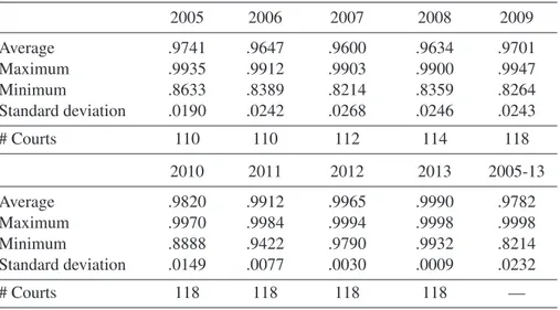
Table 4: DESCRIPTION OF EFFICIENCY LEVELS(%) FOR PERIOD(2005-13): CIVIL COURTS OF FIRST INSTANCE(MODEL4, TABLE2)
2005 2006 2007 2008 2009 Average .9741 .9647 .9600 .9634 .9701 Maximum .9935 .9912 .9903 .9900 .9947 Minimum .8633 .8389 .8214 .8359 .8264 Standard deviation .0190 .0242 .0268 .0246 .0243 # Courts 110 110 112 114 118 2010 2011 2012 2013 2005-13 Average .9820 .9912 .9965 .9990 .9782 Maximum .9970 .9984 .9994 .9998 .9998 Minimum .8888 .9422 .9790 .9932 .8214 Standard deviation .0149 .0077 .0030 .0009 .0232 # Courts 118 118 118 118 —
Source: Own elaboration.
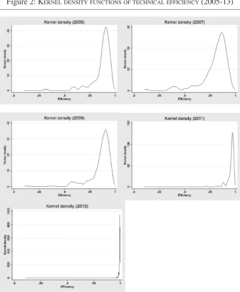
According to the estimates obtained from Model 4, the average efficiency value increased over time (from 0.9741 to 0.9990), and most importantly, dispersion in levels of efficiency tended to vanish in the last period of our sample29. This is more
readily verifiable in Figure 2, where the distribution function of the efficiency ratio is shown for every two years. Overall, we can conclude that the falling trend in the resolution ratio shown in section 2.1 (Figure 1) till 2008 (minimum) was not due to decreasing efficiency, but rather to an increase in the amount of litigation (a factor picked up by N), which was not matched by a corresponding increase in supply (i.e., congestion). Since then on, the resolution ratio increases again due to a combination of increasing efficiency and lower congestion30.
Figure 2: KERNEL DENSITY FUNCTIONS OF TECHNICAL EFFICIENCY(2005-13)
Note: Calculated from results provided by Model 4 (Table 2). The range of values on the x-axis is common to all years (0.82-1).
3. CONCLUSIONS
In this paper, we have sought to assess the performance of the civil courts of first instance. Based on our efficiency estimates, which are increasing along time, the poor performance of the justice administration can only be due to an increasing level of litigation (congestion). Hence, this points to the need to somehow regulate access to the justice system and/or to increase the number of courts.
In contrast to previous studies, here, in conducting our analysis we have been able to take advantage of a panel of data –which has allowed us to verify the evolution in efficiency levels over time, as we already suggested in the previous paragraph– and of a stochastic frontier analysis –which has enabled us to conduct a consistent estimation of the explanatory factors of efficiency–. Among these factors, we have identified the negative impact of the percentage of temporary judges and of the percentage of tem-porary court secretaries. Thus, inefficiency tends to increase the greater the number of days these positions are filled by temporary staff. As regards future research, it would be interesting to apply this type of analysis to the universe of Spanish courts.
REFERENCES
Acemoglu, D., James, S. and J. Robinson (2005): “Institutions as the Fundamental Cause of Long-Run Growth”, in Handbook of Economic Growth, P. Aghion and S. Durlauf (edi-tors), pp. 385-472, Elsevier, North Holland.
Barro, R.J. (1997): The Determinants of Economic Growth: A Cross-Country Empirical Study, MIT Press, Cambridge.
Beenstock, B. and Y. Haitovsky (2004): “Does the appointment of judges increase the out-put of the judiciary?”, International Review of Law and Economics, vol. 24, pp. 351-369. Calvo, M., Gascón, E. and J. Gracia (2004): “El tratamiento de la inmigración en la Admin-istración de Justicia”, en Justicia, Migración y Derecho, pp. 175-189, L. Miraut (Editor), Dykinson, Madrid.
Christensen, R.K. and J. Szmer (2012): “Examining the efficiency of the U.S. courts of ap-peals: Pathologies and prescriptions”, International Review of Law and Economics, vol. 32, pp. 30-37.
Coelli, T.J., Rao, D.S.P., O’Donnell, C.J. and G.E. Battese (2005): An Introduction to
Effi-ciency and Productivity Analysis, 2nd Edition, Springer, New York.
Coelli, T.J., Perelman, S. and E. Romano (1999): “Accounting for Environmental Influences in Stochastic Frontier Models: With Application to International Airlines”, Journal of
Pro-ductivity Analysis, vol. 11, pp. 251-273.
Deyneli, F. (2012): “Analysis of relationship between efficiency of justice services and salaries of judges with twostage DEA method”, European Journal of Law and Econo
-mics, vol. 34, pp. 477-493.
Dimitrova-Grajzl, V., Grajzl, P., Sustersic, J. and K. Zajc (2012): “Court output, judicial staffing, and the demand for court services: Evidence from Slovenian courts of first in-stance”, International Review of Law and Economics, vol. 32, pp. 19-29.
Di Vita, G. (2010): “Normative complexity and the length of administrative disputes: evidence from Italian regions”, European Journal of Law and Economics, vol. 34, pp. 197-213. EEAG (2011): The EEAG Report on the European Economy, “Spain”, pp. 127-145, CESifo,
Munich.
E
A
Esteller-Moré, A. (2002): “La configuración de una tasa judicial: análisis teórico”,
Investi-gaciones Económicas, vol. 26, pp. 525-549.
Fried, H.O., Knox Lovell, C.A. and S.S. Schmidt (2008): “Efficiency and Productivity”, in
The Measurement of Productive Efficiency and Productivity Growth, pp. 3-91, H.O.
Fried, C.A. Knox Lovell. S.S. Schmidt, Oxford University Press.
García-Rubio, M.A. and V. Rosales-López (2010): “Justicia y Economía: Evaluando la Eficiencia Judicial en Andalucía”, InDret, Revista para el análisis del Derecho, vol. 4, October. Gravelle, H. (1990): “Rationing Trials by Waiting: Welfare Implications”, International
Re-view of Law and Economics, vol. 10, pp. 255-270.
Greene, W. (2005): “Reconsidering heterogeneity in panel data estimators of the stochastic frontier model”, Journal of Econometrics, vol. 126, pp. 269-303.
Kittelsen, S.A.C. and F.R. Førsund (1992): “Efficiency analysis of Norwegian district courts”,
Journal of Productivity Analysis, vol. 3, pp. 277-306.
Koopmans, T.C. (1951): “An Analysis of Production as an Efficient Combination of Activi-ties”, pp. 33-97, in Activity Analysis of Production and Allocation, T.C. Koopmans (Ed-itor), Cowles Commission for Research in Economics, Monograph #13, Wiley, New York. Kumbhakar S.C. and C.K. Lovell (2000): Stochastic Frontier Analysis, Cambridge
Univer-sity Press, Cambridge.
Neyman, J. and E.L. Scott (1948): “Consistent estimation from partially consistent observa-tions”, Econometrica, vol. 16, pp. 1-32.
North, D. (1990): Institutions, institutional change and economic performance, Cambridge University Press, Cambridge.
Pastor, S. (2003a): “Eficacia y eficiencia de la justicia”, Papeles de Economía Española, vol. 95, pp. 272-305.
Pastor, S. (2003b): “Dilación, eficiencia y costes. ¿Cómo ayudar a que la imagen de la Justicia se corresponda mejor con la realidad?”, Documento de trabajo nº 5, Fundación BBVA. Pedraja, F. and J. Salinas (1996): “An assessment of the efficiency of Spanish Courts using
DEA”, Applied Economics, vol. 28, pp. 1391-1403.
Priest, G.L. (1989): “Private litigants and the court congestion problem”, Boston University
Law Review, vol. 69, pp. 527-559.
Ramello, G.B. and S. Voigt (2011): “Introduction”, Special Issue of the International Review
of Law and Economics on The Economics of efficiency and the judicial system, vol. 32,
pp. 1-2.
Ramseyer, J.M. (2012): “Talent matters: Judicial productivity and speed in Japan”,
Interna-tional Review of Law and Economics, vol. 32, pp. 38-48.
Rosales-López, V. (2008): “Economics of court performance: an empirical analysis”,
Euro-pean Journal of Law and Economics, vol. 25, pp. 231-251.
Schneider, M.R. (2005): “Judicial Career Incentives and Court Performance: An Empirical Study of the German Labour Courts of Appeal”, European Journal of Law and Economics, vol. 20, pp. 127-144.
Simar, L. and P.W. Wilson (2007): “Estimation and inference in two-stage, semi-parametric models of production processes”, Journal of Econometrics, vol. 136, pp. 31-64. Tulkens, H. (1993): “On FDH efficiency analysis: some methodological issues and
applica-tions to retail banking, courts and urban transit”, Journal of Productivity Analysis, vol. 4, pp. 183-210.
Tulkens H. and P. van den Eeckaut (1995): “Non-parametric efficiency, progress and regress measures for panel data: methodological aspects”, European Journal of Operations
Vereeck, L. and M. Mühl (2000): “An Economic Theory of Court Delay”, European
Jour-nal of Law and Economics, vol. 10, pp. 243-268.
Wang, H.J. and P. Schmidt (2002): “One-Step and Two-Step Estimation of the Effects of Ex-ogenous Variables on Technical Efficiency Levels”, Journal of Productivity Analysis, vol. 18, pp. 129-144.
Wang, H-J. and Ch.-W. Ho (2010): “Estimating fixed-effect panel stochastic frontier models by model transformation”, Journal of Econometrics, vol. 157, pp. 286-296.
Yeung, L.L. and P.F. Azevedo (2011): “Measuring efficiency of Brazilian courts with data en-velopment analysis (DEA)”, IMA Journal of Management Mathematics, vol. 25, pp. 1-14.
Fecha de recepción del original: junio, 2013 Versión final: enero, 2015
RESUMEN
Inferir las causas de las diferencias entre unidades de la administración pú-blica en el desempeño de sus funciones es cuanto menos tan importante como cuantificar el propio nivel de desempeño. Identificamos dos causas: ineficiencia y congestión. La ineficiencia puede ser debida al hecho de que los inputs son de una calidad relativamente menor (por ejemplo, trabajado-res temporales) o que, dado un nivel de calidad, los inputs no tienen incen-tivos a maximizar el nivel de esfuerzo. Los problemas de congestión surgen cuando el número de nuevos casos está por encima de los que se pueden re-solver cuando el nivel de eficiencia es máximo. Esta descomposición es apli-cada al universo de juzgados catalanes de primera instancia para el período 2005-13 aplicando un modelo de frontera estocástica con efectos fijos de pa-nel (Wang and Ho, 2010). De nuestro análisis, se concluye que el nivel de desempeño no es bajo a consecuencia de ineficiencia técnica por parte de los juzgados, sino al incremento en la litigiosidad, esto es, debido a la con-gestión, mientras que la ineficiencia tiende a disminuir a lo largo del tiempo y está correlacionada con la presencia en los juzgados de jueces sustitutos.
Palabras clave: juzgados de primera instancia, eficiencia técnica,
análi-sis de frontera estocástica, datos de panel.