Analysing monetary and fiscal policy regimes using deterministic and stochastic simulations

(1)

Economics Department

Analysing Monetary and Fiscal Policy Regimes Using Deterministic and Stochastic Simulations

R

ay

B

arrell

, K

aren

D

ury and

I

an

H

urst

ECO No. 99/37

EUI WORKING PAPERS

WP

330 EUR

(2)

q n n n i mi ni J 0001 0038 5336 5 © The Author(s). European University Institute. version produced by the EUI Library in 2020. Available Open Access on Cadmus, European University Institute Research Repository.

(3)

EUROPEAN UNIVERSITY INSTITUTE, FLORENCE ECONOMICS DEPARTMENT

WP 330

EUR

EUI Working Paper ECO No. 99/37

Analysing Monetary and Fiscal Policy Regimes

Using Deterministic and Stochastic Simulations

R

ay

B

arrell

, K

aren

D

ury

and

I

an

H

urst _©The Author(s). European University Institute. version produced by the EUI Library in 2020. Available Open Access on Cadmus, European University Institute Research Repository.

(4)

No part of this paper may be reproduced in any form without permission of the authors.

European University Institute Badia Fiesolana I - 50016 San Domenico (FI)

Italy © The Author(s). European University Institute. version produced by the EUI Library in 2020. Available Open Access on Cadmus, European University Institute Research Repository.

(5)

Analysing Monetary and Fiscal policy regimes using

deterministic and stochastic simulations

Ray Barrell, Karen Dury and Ian Hurst National Institute of Economic and Social Research

2 Dean Trench Street Smith Square

London SW1P3HE

Rharrell@ntesr.ac.uk. K.Durv (fflnicsr.ac.uk

Abstract

We wish to analyse the new rules in the European fiscal and monetary environment, and to investigate the effects of fiscal and monetary activism in Europe. The new European Central Bank has to decide on its monetary policy stance and we aim in this paper to contribute to the debate on the best overall policy rule for Euroland. We discuss the types of rules that the Bank may consider implementing and their effectiveness in stabilising individual economies. We look at policy options under our preferred rule, and we undertake stochastic simulations on the National Institutes Global Econometric Model, NiGEM, in order to evaluate different parameterisations of the rules. © The Author(s). European University Institute. version produced by the EUI Library in 2020. Available Open Access on Cadmus, European University Institute Research Repository.

(6)

(7)

Fiscal and Monetary Policy in Europe

The European Union economies have embarked on a programme of economic transformation that changes their mode of governance. Rules for monetary policy making have been fundamentally altered for 11 of them, and all 15 are variously bound by Treaty or Protocol to fiscal programmes that have significant implications for the flexibility with which they operate stabilisation policy.

We start with a brief discussion of the policy environment, and then look at stochastic simulations and at the structure of the model, NiGEM. We then discuss monetary policy in EMU and the possibilities facing the ECB and the central banks outside EMU. We look at the potential variability of inflation in the EMU area and the possibility of exceeding the potential target bounds. The paper then discusses the fiscal policies of the individual countries, both in terms of their current commitments and the prospects for improvement. We then look at estimates of the variability of output and the effects of output on deficits in order to evaluate the possibilities that the Stability Pact and Maastricht guidelines may be breached. We then look at two forms of analysis of fiscal policy. We briefly discuss some results from stochastic simulations under different monetary policy rules using our model, Nigem, and in an Annex we undertake some deterministic simulations that we think represent the policy options that must be discussed in Europe at present.

The Policy Environment

We argue that the policy responses employed by the authorities will have direct consequences for the overall effects of a stochastic sequence of shocks, and hence we cannot isolate the effects of the change from that response without undertaking further analyses of the effects of different parameterisations of feedback rules. We focus on combining a standard monetary policy rule, where the central bank targets some monetary or nominal aggregate, with elements of an inflation targeting regime and we also look at a pure inflation targeting regime.

A typical policy for a central bank may be to target some nominal aggregate such as nominal GDP or the money stock. We use these terms as substitutes for each other, as a velocity de trended monetary aggregate will move in line with nominal GDP in the medium term, and as we are not assuming that the authorities wish to hit their target period by period, responses will be similar with either target. A standard monetary policy rule would be to change the interest rate according to some proportion of the deviation of the targeted variable from its desired path. For example a proportionate control rule on the money stock would be:

r, = ^ P , Y , - P * , y,*)

(

1 )

where P = Price level and Y is real output with an asterix denoting target variables. However, a nominal target only stabilises inflation in the long run and policy makers are likely to be concerned with keeping inflation at some desired level in the short tenm. During the 90’s several countries, including the UK and New Zealand have moved to a new monetary policy regime of inflation targeting and have announced a formal inflation targeting framework. The target for the UK is 2.5% per annum, although the details of the targeting regime are not announced, and hence markets have to form judgements. We might write a similar rule as (1) with the money stock

(8)

replaced with the inflation rate. This would give a simple proportional rule on the inflation rate:

r, = y 2(AP, - AP,*) (2)

It appears from Duisenberg (1998) that the ECB will adopt a combination of these two approaches. Here we assume the ECB will adopt a combined rule of nominal GDP (as opposed to the money stock) and inflation rate targeting for reasons mentioned above. This gives:

r, = y l ( P , Y , - P * , Y,*) + y 2( AP, - AP, * ) (3)

This can be re-written as

r, = y n {P, - P * , ) + y l2{Y, - Y * , ) + y 2( A P , - A P , * ) (4)

where yn = Y12 for nominal targeting.

The rules used in this paper use the Consumer Price Index (CPI) inflation rate as a target.1 In each rule we look at we are targeting the current rate of inflation and the current level of a nominal magnitude. It is argued that a measure of forecast inflation is more appropriate due to the lag in monetary policy affecting the economy2. However we believe it is likely that the ECB is actually reacting to current conditions and it is also the case that in a forward looking model current conditions are in part reflecting future outturns. For these reasons we concentrate on using current

deviations from target in our rules. The coefficient on the nominal aggregate, yu/12 , in

the target rule was initially derived by inverting the long run solution to estimated standard money demand equations, with r, the nominal short-term interest rate being put on the LHS

r = M P Y

-c c c

where M is the nominal money target (nominal money supply) and PY is nominal domestic output. This can be simplified to:

r = -y,[nominalmoney stock target- nominal K|

substituting the money stock target with a nominal GDP target, we get: r - -y JN o m in a lf target- nominalT]

where yi is the strength of feedback. This can be altered to speed up or slow down adjustment. The coefficient on the inflation target is set at l.3 The three rules considered in this paper are fully nested in equation 4. They are:

RULE 1: Nominal GDP targeting (yn = yi2 > 0)

RULE 2: Nominal GDP targeting + inflation targeting (yn = yu > 0 and jz = 1) RULE 3: Pure inflation targeting. (y2 = 1)

' Issues arising from targeting the domestic inflation rate (where only inflation in the domestic component of the CPI, or GDP deflator) is targeted are dealt with in Svensson (1998). ! See Svensson 1997

3 In another paper by Barrell, Dury and Hurst (1999), further parameterisations of the rules are explored and the issue of the size of coefficient on the inflation rate is discussed. We also demonstrate that in models with real balance effects a coefficient of one on the feedback rule is stabilising.

(9)

A single monetary policy is applied to the Euro wide area in that interest rates do not react to individual country developments but to EMU wide aggregates. The United Kingdom is not in EMU and so follows its own interest rate reaction function and the results reported for the UK reflect the effect of changing the UK monetary policy rule. Denmark is not in EMU but has declared that it will follow EMU monetary policy and so the results for Denmark are the effects of changing the monetary policy rule in EMU. Denmark is also used in calculating the EMU aggregates. Sweden and Greece are also out of EMU and their individual policy rule is left unchanged across the stochastic simulations. Therefore results for these countries reflect changes to other country policy rules.

The Model

NiGEM is an estimated model that uses a ‘New-Keynesian’ framework in that agents are presumed to be forward-looking but nominal rigidities slow the process of adjustment to external events. The theoretical structure and the relevant simulation properties of NiGEM are described in Barrell and Sefton (1997) and NIESR (1998). The model contains estimated structures for the whole world, with the major economies having 60-90 equation models with around 20 key behavioural equations. It has complete demand and supply sides, and there is an extensive monetary and financial sector. All countries in the OECD, including South Korea, are modelled separately, as is China. There are regional blocks for East Asia, Latin America, Africa, Miscellaneous Developing countries, and Developing Europe.

Short term interest rate changes should have an impact on long term interest rates, equity prices and exchange rates. NiGEM is most commonly used for scenario analysis under the assumption that expectations in financial markets are rational, in that they are fully consistent with the outcomes of an event given the reactions of policy makers. Hence financial variables can 'jump' in the first period of a scenario. These assumptions are adopted here. An anticipated and sustained fall in interest rates in Japan, say, will cause the Yen/dollar rate to jump in the first period4. The size of the jump depends upon the interest differential that opens up. The anticipation of lower short-term rates will cause long-term rates to fall by the forward convolution of short term interest rate changes. Equity prices will rise when interest rates are anticipated to fall. Hence any shock that is expected to slow down activity will have its effects partly offset by the automatic shock absorbers in the monetary system. The size of the effect will depend upon the monetary rules used by the authorities.

Forward looking long rates have to look T periods forward

1) (l+LR,) = nj=1,T(l+SRltj)T

Forward looking exchange rates have to look one period forward 2) RX, = RX,+i (1 +SRH,)/( 1 +SRFt)

Terminal conditions are needed - a rate of growth of RX terminal condition is applied. These variables can ‘jump’ in the first period of the run

The forward-looking nature of these markets is central to model properties. The model is solved in a sequence of loops, utilising the sparse structure of forward links in time. A shock is applied, and the model is run over the full time period, and interest rates are allowed to be endogenous. A fall in demand will, for instance, cut interest rates.

4 The forward solution utilises a version of Fan/Taylor.

(10)

Forward looking agents know this, and we emulate this knowledge by running the model a second time, but calculating the long rate as the forward convolution of short rates in the previous run. The model is continually run forward and starts again, and this is repeated until a solution is found where rates of growth of expected variables are constant at the terminal date, and all equations are converged.

Policy rules are important in ‘closing the model’ and we have them for fiscal and monetary policy. We assume budget deficits are kept within bounds in the longer term, and taxes rise to do this. This simple feedback rule is important in ensuring the long run stability of the model. Indeed, as Blanchard, 1986, shows, without a solvency rule (or a no Ponzi games assumption) there is no solution to a forward-looking model. We can describe the simple fiscal rule as

Tax, = Tax,.i + <|p[T - S]

Where Tax is the direct tax rate, and T and S are the government surplus target and actual surplus respectively, and $ is the feedback parameter designed to remove an excess deficit in less that five years.

In our analyses labour markets are assumed to embody rational expectations, at least where we have evidence that bargainers use forward expectations, much as in Anderton and Barrell (1995). However, consumers are not assumed to look forward when making their decisions today. This does not mean that future events do not affect their behaviour, as forward looking long rates and equity prices affect debt interest payments and asset values now. Hence financial markets bring forward the consequences of future events, acting as ‘agents’ for more passive households. Changing to forward looking household behaviour does not affect our results in any significant way. The model is large, but with a common (estimated and calibrated) underlying structure across all economies. The whole model is solved simultaneously in forward mode.

The speed of adjustment of wages and prices is estimated to vary between countries, and depends upon institutions in the labour and product markets. In general the US and the UK react more quickly to excess capacity than do the more regulated continental European markets, and our results reflect these differences. There arc also differences in speeds of adjustment in personal sector consumption, as well as differences in the underlying structure of wealth and hence its effects on consumption. Stochastic simulations

The most common way to evaluate the robustness of policy is to undertake stochastic simulations, and the techniques we use are fully detailed in Barrell, Dury and Hurst (1999a). Within this framework, a variety of shocks are imposed on the model. These shocks are taken at random from a particular distribution and are repeatedly applied to the model. Hence the moments of the solution of the endogenous variables can be calculated and uncertainty investigated. Stochastic simulation can be either in respect to the error terms, coefficient estimates or both. In this paper we assume that the coefficient estimates are known with certainty and the stochastic shocks to the model are only applied to the error terms, much as in the rest of the economic literature. We use the boot strap method where the shocks are generated by repeatedly drawing random errors for individual time periods for all equations from the matrix of single equation residuals (SER). The shocks drawn will have the same contemporaneous distribution as the empirical distribution of the SER, which is assumed to be normally

(11)

distributed, N(0,a2). In this way the historical correlations of the error terms is maintained across variables, but not through time. If, for example, investment shocks across Europe are highly positively correlated, the error terms will tend to be high together for these countries. There are a number of other methods for drawing the shocks which rely on specifying the variance-covariance matrix or generating pseudo random shocks which are consistent with the historical residuals.

Monetary Policy in The Euro Area

On January Is', EMU began its third stage, and eleven European economies entered into a monetary union. This occurred under relatively favourable economic conditions. All countries except Italy were expected to have grown by more than 2Vi per cent in 1998; and inflation is at historically low levels. The Euro Area fiscal deficit is below 3 per cent of GDP; Euro Area government debt is approximately 75 per cent of GDP, having declined for three years in succession, and the launch was surrounded by a general optimism. Co-ordinated rate cuts in early December ensured short-term interest rate convergence. Only Italy maintained an interest rate differential following these cuts, and this was eliminated by the end of December. The initial key repo interest rate of the European Central Bank stands at 3 per cent. This rate was cut to 2.5 percent in April 1999

European-wide financial markets are already being created, but their regulation is likely to be largely left to the discretion of the national authorities. All government bonds of the member countries were re-denominated into Euros prior to the first trading day of 1999. Some very short-term debt was exempt from re-denomination, although all new debt must now be issued in Euro. Some private bonds will also be re denominated, although there is no requirement to do so until January 1, 2002. There is no explicit reference in the Maastricht Treaty to a lender of last resort role for the ECB. The banking system is regulated at the national level, and in banking crises the individual Central banks would have to step in to provide liquidity in their country. However, this may put pressure on the liquidity of the whole European market, and hence the ECB may well still have to act as a lender of last resort for the provision of short-term liquidity, in order to promote the smooth operation of payment systems. The fixed exchange rate in itself does not represent a sharp deviation in policy commitments, as all have been members of the Exchange Rate Mechanism for several years. The most significant change is that monetary policy decisions have been handed over to the European System of Central Banks (ESCB). This consists of the ECB and the Central Banks of all countries in the EU. The ESCB will maintain control over key interest rates, reserve ratios, foreign exchange operations and central bank money. National central banks will be responsible for carrying out the monetary policy decisions and hence intervening in domestic financial markets to ensure that asset prices are at levels that will sustain the interest rate decisions of the ESCB. The primary goal of the ESCB is to maintain price stability in the Euro Area, defined as a year-on-year increase in the Harmonised Index on Consumer Prices of less than 2 per cent. The dominant monetary policy strategy will be to monitor the growth of Euro M3 relative to a reference value, currently set at an annualised rate of 4Vi per cent. The policy is complicated by the fact that not all countries have regularly published comparable money aggregates, so the target has no historical reference. The M3 aggregate includes cash and bank deposits, repurchase agreements, money market fund units and short-term debt certificates issued up to 2 years. The ESCB will make a broadly based assessment of the outlook for price developments using a

(12)

variety economic and financial indicators. It will assess developments in the dollar exchange rate, producer prices and commodity prices, and may react to increases and decreases in inflation that seem initially unrelated to monetary developments. This mixed targeting rule differs a little from that explicitly adopted by the Bundesbank, and is partly designed to take account of the uncertainties in financial environment. With inflation remaining below 1 per cent in the Euro Area, and activity having begun to slow significantly, the ECB cut interest rates by 50 basis points in mid-April. The objective of the ECB is to hold inflation within a range of 0-2 per cent, implying that action will be taken to avoid the prospect of outright deflation. Clearly there were worries that inflation might fall too far in the near future, and hence the ECB acted. Table 1. Impact of Vi per cent rate cut on GDP

Per cent difference from base

Germany France Italy Spain Neths. Belgium Finland Portugal

1999 0.34 0.15 0.14 0.29 0.26 0.28 0.19 0.19 2000 0.36 0.27 0.27 0.45 0.29 0.26 0.28 0.19 2001 0.26 0.27 0.26 0.38 0.24 0.21 0.2 6 0.18 2002 0.15 0.21 0.18 0.22 0.19 0.18 0.23 0.17 2003 0.07 0.12 0.09 0.06 0.15 0.16 0.19 0.16 2004 0.02 0.03 0.00 -0.05 0.13 0.14 0.15 0.15

Austria Ireland UK Denmark Greece Sweden E U 11 EU15

1999 0.30 0.23 -0.07 0.20 -0.39 -0.10 0.24 0.17 2000 0.25 0.29 -0.04 0.26 -0.51 -0.11 0.31 0.23 2001 0.23 0.19 -0.01 0.29 -0.31 -0.04 0.26 0.21 2002 0.21 0.11 0.03 0.32 0.00 0.02 0.18 0.16 2003 0.19 0.07 0.05 0.35 0.25 0.05 0 .10 0.10 2004 0.16 0.06 0.06 0 .36 0.36 0.05 0.04 0.05

Table 2. Impact of Vi per cent rate cut on inflation

Percentage points difference from base

Germany France Italy Spain Neths. Belgium Finland Portugal

1999 0.06 0.07 0.16 0.02 0.07 0.07 0.11 0.05 2000 0.14 0 .10 0.11 0.08 0.19 0.23 0.15 0.12 2001 0.31 0.13 0.23 0.19 0.19 0.17 0.16 0.13 2002 0.32 0.19 0.28 0.25 0.17 0.12 0.16 0.13 2003 0.22 0.23 0.25 0.22 0.14 0.12 0.15 0.12 2004 0.11 0.21 0.16 0.15 0.12 0.11 0.13 0.12

Austria Ireland UK Denmark Greece Sweden EU11 EU15

1999 0.07 0.21 -0.07 0.06 -0.07 -0.02 0.08 0.05 2000 0.16 0.27 -0.04 0.18 -0.21 -0.08 0.13 0.08 2001 0.17 0.21 -0.02 0.21 -0.23 -0.10 0.22 0.16 2002 0.16 0.13 0.00 0.18 -0.14 -0.04 0.25 0.18 2003 0.15 0.06 0.01 0.19 0.00 0.04 0.21 0.17 2004 0.13 0.04 0.02 0.21 0.11 0.07 0.15 0.12 © The Author(s). European University Institute. version produced by the EUI Library in 2020. Available Open Access on Cadmus, European University Institute Research Repository.

(13)

There are several avenues through which a loosening of monetary policy can affect real activity. In a forward-looking model such as NiGEM it is common to find that a reduction in interest rates is associated with an initial depreciation of the nominal, and hence the real, exchange rate. We generally find that a Vi per cent cut in interest rates is associated with an initial depreciation of 1 per cent in the real exchange rate. In the table 1 we report the results of a simulation of the effects of the 50 basis point reduction in the Euro Area nominal short-term interest rate. We shock the nominal interest rate by -Vi point for 2 quarters and shift the monetary target of the ECB by the amount required to validate the shock. If we failed to do this, and left the money target unchanged, the ECB would in effect be reversing its monetary expansion after the first two periods. This impact is temporary, with the real exchange rate returning towards base over a few years, but it will provide a temporary boost to export demand while curbing imports. Lower interest rates also encourage investment by reducing the cost of capital, it also stimulates construction, and temporarily increases consumption through the impact of higher equity prices on wealth.

The interest rate cut raises Euro Area output above its baseline by about ‘A per cent over the first 3 years. As the baseline involves a return to full capacity output in the long run, the simulation returns to the same place and hence the effects are transitory. Germany experiences the largest initial effect on GDP, rising by over 0.3 per cent from its baseline in the first year, largely because it is more open to trade with the rest of the world than are the other major economies. The impact on Italy is weaker in the first year, although it is likely to accelerate in 2000. Apart from Germany, Spain, Belgium, Netherlands and Austria are expected to experience effects on GDP above the EU11 average. GDP is slower to react in France. Without complimentary cuts in interest rates, a contractionary effect is likely to be felt in those EU countries outside monetary union as their exchange rates are likely to appreciate against the Euro. Denmark’s exchange rate is tied to the Euro, and so we assume that interest rate movements in the Euro Area will be mirrored in Denmark.

The monetary stimulus produces a price level that is one percent higher than it would have otherwise been in the long run as compared to our baseline. Hence the impact on inflation has to be limited, although it is expected to accelerate over the next four years, with an increase of V* percentage points expected in 2002. The Euro area would remain comfortably inside the 0 to 2 per cent target range that the ECB has set itself. The strongest impact is likely to be felt in Ireland and Italy, where inflation levels are already high relative to the rest of the Euro Area. This is, of course, the risk attached to monetary loosening. A strong impact on Germany, where inflation is exceptionally low, is likely to be felt only after two years. A welcome negative impact in inflation will be felt in Greece, whereas the negative impact on Sweden is less desirable, as inflation in Sweden is running below the lower band of the central bank’s target. However, pre-emptive interest rate cuts by the Swedish central bank are likely to have counter-balanced this impact.

Evaluating Monetary Policy by Stochastic Simulations

We have argued that we should not only evaluate monetary policy by its deterministic effects. Policies are designed to deal with uncertainty, and we need to be sure that they are robust across a range of different outcomes. There is a choice to be made between rules in the Euro area, and we want to compare a simple money stock based rule with the same rule augmented by a feedback on current inflation and also a pure inflation targeting rule. Table 3 presents variabilities for short term interest rates under

(14)

the three different rules. Table 4 presents individual country inflation variabilities and inflation variability for the Euro area as a whole. The summary statistic given in the following tables are the root mean squared deviations (RMSDs)5.

Table 3: Root Mean Squared Deviations (RMSDs) for interest rates. RULE 1 RULE 2 RULE 3

Short rates UK 0.20 0.78 0.76 EL 0.70 1.28 1.23 Long rates EL 0.10 0.11 0.10 UK 0.10 0.08 0.07

We have undertaken over 200 replications on each rule, where each replication represents a complete set of forward looking runs over 20 quarters. Hence we have over 4000 observations upon which to base our comparisons of the rules, and hence we can test for differences between them. The ratio of two variances is distributed as an F statistic with degrees of freedom associated with the number of sample points. If we form the ratio of the larger variance over the smaller one we have a valid test. We may say that if variances differ by more than 6 to 7 percent then they are significantly different from each other. Each table reports the ratios of the RMSDs for each of the rules we have used in our experiments and indicates where the variances are significantly different from Rule 1 (*) and where the variances are significantly different from Rule 2 (#).

Table 4: Root Mean Squared Deviations (RMSD) of inflation RULE 1 =100

RULE 1 RULE 2 RULE 3 RULE 2 RULE 3

GE 1.33 1.18 1.15 88.72* 86.47* FR 0.82 0.76 0.67 92.68* 81.71*# SP 1.12 1.06 1.03 94.64* 91.96* IT 1.23 1.02 0.94 82.93* 76.42*# NL 1.05 1.01 0.99 96.19* 94.29* BG 1.97 1.87 1.86 94.92* 94.42* PT 2.38 2.03 1.71 85.29* 71.85*# IR 1.16 1.03 1.01 88.79* 87.07* FN 0.85 0.81 0.79 95.29* 92.94* OE 2.29 2.02 1.82 88.21* 79.48*# EL 0.78 0.76 0.79 97.44 101.28*# DK 1.42 1.38 1.33 97.18 93.66*# SD 2.06 1.78 1.54 86.41* 74.76*# GR 2.27 2.08 1.7 91.63* 74.89*# UK 0.79 0.68 0.58 86.08* 73.42*# © The Author(s). European University Institute. version produced by the EUI Library in 2020. Available Open Access on Cadmus, European University Institute Research Repository.

(15)

Table 3 shows that the reaction of the short-term interest rates increases substantially for all countries as a direct inflation target is added to a nominal magnitude based rule. For the EMU member states the volatility of the interest rate almost doubles and for the UK it is over 3 times that under Rule 1. The removal of the nominal magnitude from the rule as we move from 2 to 3 decreases variability, albeit slightly, in all cases. Under Rule 2 the variability of the long rate for the Euro Area increases but by only 10%. Rule 2 substantially increases the variability of the short rate but the long rate doesn’t increase nearly as much because of their forward looking nature on the model. Long rates are the forward convolution of the short rates and look forward 40 periods (i.e.10 years) which is further than the period over which we apply shocks in the simulations. The rule may increase the volatility of the short rates in the short run but over the medium and longer run inflation under the combined rule may be settling down a lot quicker causing long rates to be less variable over the simulation period. We have followed common practice, as in Masson and Symansky (1993) and Fair (1998) for instance, and not shocked the exchange rate. For a large relatively closed economy such as the Euro area this is not particularly important as an assumption, as we show in Barrell, Dury and Hurst (1999a). Inflation variability in the Euro area rises by around six percent if we shock exchange rates, but by fifty percent in the UK, which is much smaller and more open to the rest of the world. Not shocking the exchange rate also means we can elide the issue of defining shocks to the Euro, a currency that did not exist in our historical period. Table 4 shows that the combined rule with a coefficient of 1.0 on inflation appears to be slightly better for the Euro Area in terms of reduced inflation variability than a nominal targeting rule. A pure inflation targeting rule with the same coefficient appears to increase inflation variability.

It is interesting that under the combined rule, each individual country appears to benefit more than the Euro area does as a whole and that under the inflation targeting rule, while each country benefits, inflation variability for the Euro area actually increases. This implies that the covariance structure of Euro area changes over the different rules, as the variance of a sum (the Euro aggregate) is the weighted sum of the variances and covariances where the weights are squares or products of those used in constructing the aggregate. Denmark, Sweden and Greece all benefit from the ECB using a combined rule and benefit further from a pure inflating targeting rule. The table shows that the ECB may be indifferent between the nominal GDP rule and the combined rule as the variance is not significantly different, but would not prefer the pure inflation targeting rule over the nominal GDP or combined rule as the variance is significantly higher. However the variance is still lower under Rule 2 than Rule 1 and at a higher significance level it may prove to be the preferred rule. Individual member countries would seem to prefer the combined rule to Rule 1 and France, Italy, Portugal and Austria appear to prefer the pure inflation targeting rule above the other rules. Variances for Germany and Spain under Rule 3 are only just insignificantly different from those of Rule 2 and so it seems that there could be a strong support for a pure inflation targeting rule from individual countries. This could cause a potential conflict between the ECB and the ECB council with the former preferring either a nominal GDP or combined rule and the latter preferring a pure inflation targeting rule. The ECB has set itself the task of keeping inflation within the 0 to 2 percent band, but it has not been absolutely clear that this band is symmetric or that it is centred on one. This lack of clarity may be important for the future of monetary policy in Europe. However, we have used a forecast base where inflation is in the upper half of this

(16)

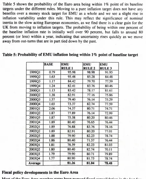
band in almost all periods (much as it has been for 30 years) and hence we feel that it is more valuable to assess the risks of being within one percent of our baseline. Table 5 shows the probability of the Euro area being within 1 % point of its baseline targets under the different rules. Moving to a pure inflation target does not have any benefits over a money stock target for EMU as a whole and we see a slight rise in inflation variability under this rule. This may reflect the significance of nominal inertia in the slow acting European economies, as we find there is a clear gain for the UK from moving to inflation targets. The probability of being within one percent of the baseline inflation rate is initially well over 90 percent, but falls to around 80 percent (or less) within a year, indicating that uncertainty rises quickly as wc move away from out-turns that are in part tied down by the past.

Table 5: Probability of EMU inflation being within 1 % point of baseline target

BASE EMU RULE 1 EMU RULE 2 EMU RULE 3 1999Q1 0.79 95.98 98.98 91.95 1999Q2 1.63 95.48 85.28 84.48 1999Q3 1.17 84.42 79.70 77.59 1999Q4 1.24 82.41 83.76 80.46 2000Q1 1.13 83.42 78.17 81.61 2000Q2 1.38 82.91 77.16 75.86 2000Q3 1.57 79.40 76.14 75.29 2000Q4 1.65 73.37 82.74 77.59 2001Q1 2.06 74.37 80.71 74.71 2001Q2 1.87 77.89 76.14 72.99 2001Q3 1.87 75.38 80.20 80.46 2001Q4 1.89 80.40 76.65 76.44 2002Q1 1.89 76.88 83.76 78.16 2002Q2 1.89 82.91 80.20 77.01 2002Q3 1.88 79.90 82.23 78.74 2002Q4 1.86 80.40 71.57 76.44 2003Q1 1.81 78.39 82.23 81.03 2003Q2 1.80 80.40 82.74 70.11 2003Q3 1.79 79.90 80.71 79.89 2003Q4 1.77 80.90 81.73 78.74 Average 81.26 81.04 78.48

Fiscal policy developments in the Euro Area

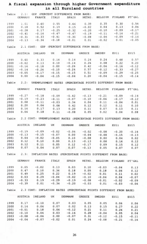
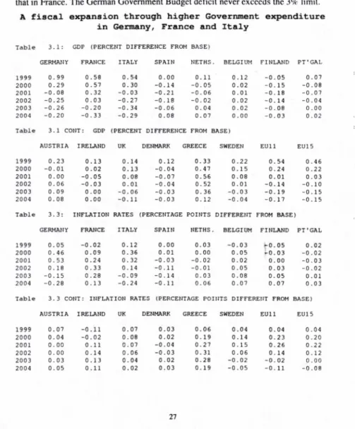
Most of the Euro Area member states have pursued fiscal consolidation in the last few years. The reduction in government deficits has generally been successful, as can be seen from Table 6, with some countries expected to run budget surpluses in 1999 and beyond. However more than half the countries may still have deficits of about 2 per cent of GDP, as special measures that were designed to achieve targets in the run up to Monetary Union are unwound. This poses the question whether current fiscal consolidation has been sufficient to remain below the reference value of 3 per cent of GDP if growth slows down more than expected. It is important to ask whether fiscal consolidation set out in various stability programmes is sufficient for all countries, or whether some governments may have to introduce additional measures.

(17)

Government expenditure in the EU declined overall in the second half of 1998. following a sharp increase in the first half of the year. This fiscal expansion was largely due to the postponement of expenditure in 1997 in order to ensure the budget deficit fell within the Maastricht criteria. The combined fiscal deficit for the Euro Area relative to GDP fell slightly in 1998, to about 2!4 per cent. We expect to see a small further reduction to 1.9 per cent of GDP in 1999. The need to meet the strict fiscal guidelines laid out in the Stability and Growth Pact is likely to continue to restrain the growth of expenditure. The four EU countries outside the monetary union are also maintaining a fairly tight or neutral fiscal policy, in accordance with the Convergence Programme guidelines of the Stability and Growth Pact. Fiscal surpluses are expected in Denmark, Finland, Ireland, and Sweden. Anticipated improvements in government finances are expected to lead to substantial reductions in the ratio of government debt to GDP over the next several years.

Table 6: Base line Government budget deficit to GDP ratios

GE FR SP IT NL BG PT IR FN OE UK 1999Q1 -2.38 -2.69 -1.48 -1.52 -1.79 -1.27 -1.78 2.65 2.55 -2.89 -0.75 1999Q2 -2.28 -2.59 -1.55 -1.89 -1.72 -0.90 -2.01 2.18 2.78 -2.59 -0.26 1999Q3 -2.27 -2.45 -1.44 -2.08 -1.53 -0.81 -1.99 2.19 2.89 -2.40 -1.12 1999Q4 -2.17 -2.33 -1.45 -2.23 -1.48 -0.73 -2.08 2.26 3.01 -2.15 -1.31 2000Q1 -2.07 -2.08 -1.32 -2.25 -1.43 -0.56 -1.97 2.33 2.88 -3.14 -1.55 2000Q2 -1.91 -1.85 -1.15 -2.27 -1.36 -0.53 -1.86 2.31 2.75 -2.45 -0.76 2000Q3 -1.77 -1.63 -0.89 -2.26 -1.26 -0.45 -1.74 2.27 2.60 -1.94 -0.57 2000Q4 -1.64 -1.42 -0.67 -2.26 -1.18 -0.44 -1.64 2.21 2.43 -1.56 -0.61 2001Q1 -1.78 -1.37 -0.43 -2.22 -1.00 -0.46 -1.44 2.22 2.37 -1.28 -0.46 2001Q2 -1.63 -1.35 -0.25 -2.11 -0.89 -0.53 -1.34 2.23 2.32 -1.08 -0.60 2001Q3 -1.47 -1.32 -0.08 -1.99 -0.79 -0.60 -1.28 2.17 2.30 -0.94 -0.60 2001Q4 -1.40 -1.28 0.05 -1.87 -0.75 -0.66 -1.25 2.07 2.29 -0.84 -0.69 2002Q1 -1.32 -1.25 0.21 -1.77 -0.70 -0.66 -1.18 1.98 2.26 -0.76 -0.72 2002Q2 -1.24 -1.21 0.11 -1.69 -0.67 -0.66 -1.14 1.85 2.22 -0.71 -0.48 2002Q3 -1.18 -1.19 0.00 -1.63 -0.65 -0.67 -1.14 1.70 2.16 -0.69 -0.44 2002Q4 -1.12 -1.16 -0.10 -1.59 -0.65 -0.68 -1.17 1.54 2.09 -0.69 -0.44 2003Q1 -1.01 -1.14 -0.18 -1.55 -0.65 -0.68 -1.19 1.38 1.91 -0.69 -0.40 2003Q2 -0.89 -1.12 -0.26 -1.64 -0.65 -0.69 -1.21 1.21 1.56 -0.68 -0.34 2003Q3 -0.78 -1.09 -0.31 -1.73 -0.64 -0.70 -1.23 1.05 1.28 -0.68 -0.31 2003Q4 -0.68 -1.07 -0.36 -1.82 -0.63 -0.71 -1.26 0.88 1.06 -0.68 -0.30

Note Base denotes our April baseline forecast for the budget deficit as a percent of GDP

Tight fiscal policy in Europe has restricted output in the short ran, and we can expect it to continue to be tightened, especially in the larger countries. The Stability and Growth Pact puts clear limits on the size of deficits that can be run, and has a rather loose fines system associated with it. Each European country has an announced Stability Pact Programme, and details of these are summarised in appendix 2 and our forecast for deficits for each member state are given in Table 6 above. The pact sets a deficit of 3 percent as a floor, and if sustained deficits of 3 per cent are maintained then there is a system of fines. There are also reference values that have to be adhered to in the long run, and deficits should stay in the range 1 to 0 percent of GDP. The suitability (not optimality) of these rules depends on the stochastic environment in which the countries exist. In order to assess this we have replicated the stochastic

(18)

environment from 1993 to 1997 with 200 replications of stochastic simulations over a five year period 1999 to 2003 using our April baseline.

We can draw some reasonably strong conclusions from our results, which arc reported in Tables 7 - 9 . Under the nominal targeting rule there appears to be a 13 per cent chance of Germany breaking the 3 percent barrier in 1999. The fiscal packages and projections expected to be in place are likely to reduce the probability to around 3 percent in 2000. On the same basis the probability of the French deficit exceeding 3 per cent in 1999 was lower at around 4 per cent, dropping to around 0.1 % in 2000. The probability of the Italian deficit exceeding 3% in 1999 is around 1.5% rising to around 5% in 2000 and dropping slightly thereafter. This would suggest that there was a need for further fiscal tightening in order to stay within the guidelines with a reasonable degree of certainty.

In contrast Spain, Ireland, Portugal, Netherlands, Belgium and Finland arc all estimated to almost certainly not exceed the limit. Austria however is estimated to have a 16% chance of exceeding the 3% limit in 1999 and 2000. The UK also appears to be well within the limit required by the Treaty. This reflects both the distance of the deficit from the boundary, the volatility of output and the effects of changes in output on the budget deficit. Our estimates of these three magnitudes depend upon our base and our structural economic model, and not on historical estimates of these variances. Variability may have been large in the past because of policy mistakes rather than the innate variability associated with economic behaviour. Our results factor these mistakes out to the extent that they were associated with devaluations, and hence by not shocking their exchange rates we have avoided polluting our results for the future with the devaluation cycles seen in Finland, Sweden, Spain and Portugal. In our analysis in Barrell, Dury and Hurst (1999a) we draw our shocks from an historical synthetic exchange rate for the Euro, based on shocks to the core ERM countries, rather than take the average of the shocks to each of the exchange rates. Hence only Sweden would be shocked in relation to its historical devaluation cycle, and our results for the Euro members is probably a better representation of the future than any based on using all past data.

Under Rule 2, the combined nominal aggregate and inflation target rule, the probability of exceeding the fiscal target of a 3 percent deficit increases in all countries except for Belgium and Portugal. Under the pure inflation targeting regime, Rule 3, the probabilities increase further except for Belgium, Portugal, Austria and the Netherlands. The probabilities of a breach in 1999 rise more for France than they do for Germany as we increase the relative importance of the inflation component of the monetary targeting regime. Indeed, the change in rule increases the probability of the French breaching the guideline from 4 percent to over 11 percent in 1999. The same change in rules from targeting a nominal aggregate to targeting inflation raises the probability of an Italian breach of the guidelines from 1.5 percent in 1999 and 4.5 percent in 2000 to 5.5 percent in 1999 and nearly 14 percent in 2000. Italy is the only large country where the probability of a breach rises significantly between 1999 and 2000.

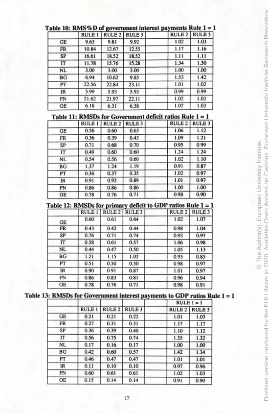
The probability of a breach depends on the variability of income and prices and on their effects on the deficits, either directly or through policy reactions such as interest rate changes. Table 10 shows that Government interest payments become more volatile under Rule 2 and 3 compared with Rule 1. The degree to which the variability in interest rates feeds through to the variability of government interest payments

(19)

depends on the structure of the debt. For example, the Italian government has issued a lot of short term debt and so the variability of the short term interest rate will substantially affect the variability of the interest payments. Detailed descriptions of the sources of potential volatility are useful in this context, and we report the components of the deficit in tables 10 to 13. Table 12 gives the variability of the primary deficit ratio. In general the variability of the primary deficit ratio is quite a lot larger than the variability of the Government interest payments ratio. Of course decomposing the variability of the overall deficit in this way we must lake into account the covariance, but the tables show that the volatility of the overall deficit ratio is mainly generated by volatility in the primary deficit ratio. Table 13 shows that interest payments become more volatile as the short term interest rate variability increases as we shift toward inflation targets. This effect is particularly significant in Italy and Belgium, both of which are high debt and high short term debt countries and so their Government interest payments are affected more by the variability of the short term interest rate. Interestingly for Belgium the sharp rise in the variability of the Government interest payments ratio does not outweigh the fall in the primary deficit ratio and the variability of the overall ratio still falls.

The pact rules on ‘near budget balance’ are obviously of interest, and Tables 1 4 - 1 6 report on the probabilities of being within the range of 0 to 1 for the deficit under all three rules. This is low in 1999 for all EMU members except for Spain, Belgium and the Netherlands under Rule 1. The UK has the highest probability of being near balance in 1999, whilst Ireland and Finland stand little chance of falling within this range as they have been running substantial surpluses and are expected to continue to do so over our horizon. The probability of being in balance or near it under Rule 1, rises for Germany, and by the end of our period has risen to around 54 percent, whilst it is around 32 percent for France, and 45 percent for Spain and 58 percent for the Netherlands.

Tables 14-16 show that for all rules, most countries improve their positions over time. The tables also show that the probabilities rise as we include a direct inflation target into the rule and rise further as we move to a pure inflation targeting rule. Charts 1 -3 show the distribution of German Budget ratios over time for Rule 2. This is as expected as feedbacks in the model bring the deficit ratio back to its baseline trajectory over time. It is interesting to look at how the distribution of results change over the different rules. Tables 7 to 9 show that, for the larger economies in EMU, the probability of exceeding the target increases as we move from Rule 1 up to Rule 3. Tables 14-16 show that the probability of being near balance increases as we move from Rule 1 to Rule 3. This implies the distribution of the results flattens out as we move up the rales. One of the countries this is particularly prevalent for is Italy. Charts 4 to 6 show how the distribution of the results spread out for Italy as we move from Rule 1 up to Rule 3 for 2001q4, the same pattern can be seen for other years but are not shown here6.

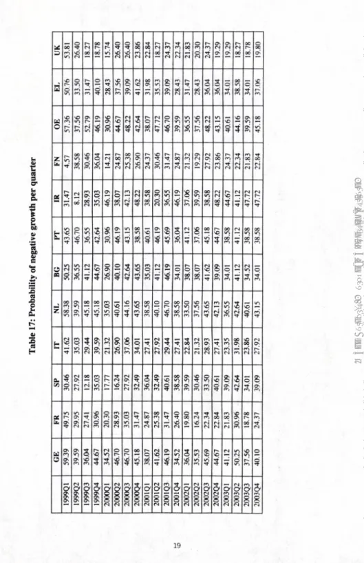
The pact cannot be seen as particularly stringent, and it has other let-our clauses for the persistently penurious. They are allowed to borrow excessively if they have moved sharply into recession or are a long way from full capacity. The possibility of negative growth for any quarter is quite high, as can be seen from Table 17. Probabilities range from 25% to 50% in 1999 and 21% to 43% for 2000. For Euroland

6 For most countries for 4 out of the 5 years the Kurtosis value falls over the rules indicating the distribution is becoming less peaked as we increase the reliance of inflation targeting.

(20)

as a whole there is around a 38% chance of having negative growth in any one quarter, and the probabilities are initially higher than this. If shocks are serially independent, as we would hope, then the trigger cause (2 quarters of income decline! could happen in about 15 percent of all cases.

Commission Based Estimates of Fiscal Breaches

Our technique uses a whole model, and shocks all stochastic equations, including the tax and expenditure equations on the model, and hence the calculations are not easily reducible to the interesting simple formulae in Buti, Franco and Ongcna (1997) or Bayar and Ongena (1998). Tables from these papers are reproduced in Annex 2 and Annex 3, and we can utilise them in order to make some preliminary estimates of the probabilities of exceeding the target deficits and then compare them with those from our model based analysis.

In order to assess the probability of a country breaching the fiscal guidelines wc need some estimates of the volatility of output and the effects of output on the deficit. Wc also need some baseline estimates of the expected deficit in order that we can put bounds around it. Bayer and Ongena (1998) have used Hodrick-Prescott filters to obtain estimates of trend output and hence of the volatility of output around trend. They use a relatively long time span, and they calculate that output is (was) most variable (as measured by its standard deviation as a percent of GDP) in Finland (2.2), Sweden (1.7), Spain (1.5) and the UK (1.4) and least variable in Italy (0.7), Austria (0.7) and France (0.8). These depend on history, the nature of automatic stabilisers and the policy reaction functions in place over the period and they may not be good indicators for the future. For instance politically induced devaluation cycles are at least part of the reason for volatile output in the first four countries mentioned, and this can explain why they have chosen to give up the exchange rate instrument and join EMU.

The effects of volatile incomes depend on the sensitivity of the budget deficit to the cycle, and these again depend upon automatic stabilisers. Buti, Franco and Ongena (1997) have calculated these for the European economies, and they suggest that a one percent of GDP fall in output causes a 0.7 percent worsening of the budget deficit in Sweden, 0.6 percent in the Netherlands and 0.5 percent in the UK, Finland and Belgium. Other countries are lower. If historical volatilities are applied to these coefficients it is clear that budget deficits would be most volatile in Sweden and Finland, much as they have been over the last 30 years.

If we have the standard deviation of output and the impact of changes in output on the budget, then we can calculate the probability that the deficit differs from baseline by any given amount. Given the targets for budget deficits in Annex 3 we can calculate the probability of the deficit exceeding 3 percent in 1999. Given this information we can say that the probabilities are around 10 percent for Spain and the Netherlands, 5 percent for Germany and France, and less for the other members. This in part reflects the fact that the historically more volatile countries are currently running budget surpluses. It is also possible to invert the question and ask, given historical volatilities, what would the target deficit have to be to reduce to 1 percent the probability of having a deficit in excess of 3 percent of GDP. The information in the tables suggests that the Finns and the Swedes would have to aim for surpluses of 2.5 percent of GDP and 1.8 percent of GDP respectively. The UK, the Netherlands (both -0.5 percent), Spain (-0.6 percent) and Denmark (-0.7 percent) should heed the Commissions desire to keep within a target range of 0 to -1.0 percent. However, the less volatile or

(21)

responsive countries could aim for larger deficits than the Stability and Growth Pact suggests. Belgium (-1.4 percent), Portugal (-1.5 percent), Ireland (-1.6 percent) and Germany (-1.7 percent) could all run reasonable deficits, and the rest of the members of EMU could aim at -2.0 percent.

Given these estimates the Pact appears to be rather tight given its initial aims. Wc should of course treat the estimates for the more historically volatile countries with caution, as they have all attempted to reduce uncertainties by either adopting an inflation targeting regime (UK and Sweden) or they have joined EMU to ensure the same thing. Given these caveats, our model based estimates are similar in many ways. Conclusions

Evaluating monetary and fiscal policy by deterministic simulations is of great value, and can suggest options that are of use in the current conjuncture. However, the evaluation of options and risks in a stochastic environment using feedback rules that can be seen as relevant is important. Stochastic simulations can also be used to search over relevant rules when deciding on the framework of governance. This paper has begun to look at these problems for the European economies, and in particular we have tried to draw some light on the possibilities of the ECB being within one percentage point of our baseline target and Individual European countries defaulting on the Stability and Growth Pact (SGP). We have found that inflation targeting does not seem to benefit the ECB in terms of helping to hit the inflation target but some form of inflation targeting can be disadvantageous for individual countries in terms of being within the criteria of the SGP. The degree to which the rule affects the probability of default depends on the variability of the short term interest rate under the rule and the size and structure of government debt. With a high proportion of debt held in short term bonds, a high variability of the short term interest rate will have a greater affect on the variability of the government budget ratio and this could increase the probability of defaulting on the SGP. The results also suggest that it may be more appropriate for the primary deficit ratio to be the target and not the overall budget ratio as this is in the control of the fiscal authorities. What happens to Government interest payments reflects the variability of short term interest rates which is in the hands of the monetary authorities. It may also be more appropriate for there to be individual targets for each member country instead of a ‘one size fits all’ fiscal

requirement. © The Author(s). European University Institute. version produced by the EUI Library in 2020. Available Open Access on Cadmus, European University Institute Research Repository.

(22)

T a b ic 7: P ro b a b il it y o f G o v e rn m e n t b u d g e t d e fi c it r a ti o ex ce e d in g 3 % u n d e r R u le 1 U K G BR m sO © m r* d m SO d n m 5 d ELGBR s d o o o 8 d W .V A 7 0 .0 0 OEGB R 1 8 0 9 1 2 1 .6 1 CTs ro (S n m - vO d d FNGBR 0 0 0 0 0 0 U V V / o o o 0 .0 0 IR GB R0 0 0 o o o 8 S d c 0.0 0 PTG BRm sO d oo 00 d 8 Sd c o o o n n * n B G GB R © PS 00 00 SC cPS n PS r< h SO n r-> r> (S NLG B R o_o o 0.13 8 § d c§ :>8d ITGB R in msC ■«t — o m n cU .JO 1 .3 8 SP GB R o o o o o o 0 .00 n n r» w .w 0 .0 0 FRGBR PS q Tf 0.13 u u u o o o § 8 d GEGBR Os rn PS q rn 00 r m - O C 2 8 i d 0 0 6 6 6 1 1 1 o o o o o z 1 8 S 8 5 cs r 4.W 4 .. W 2003 .00 & £>_ea JO c £ U K G B R 0 .89 ₁A l \ ? s - d m d m d EL G BR_{8 S} d c5 85 d o o o o o o OEGB Rin si r~~ r o r oc m d »nd FNG BR_{8 5} d c o o o n rv n o o o o o o IRG BR_{8 5} d c 0.0 0 oo o s z o PT GBR c y \ j £9 0 V.W J 0.13 o o o o o o BG GBR psin r r 3 .0 5 2 oo PS (S NLGB R 0. 38 n 7 Q ₈ d £ 1 0 rn d ITGBR 5 .08 o a n 00_in in OO f-; insC SP GB R 2 g d c 8d 0 0 0 8 d FRGBR in ps r oc c 0.0 0 00 0 o o o GE GBR10 r■*i O 12 p 1.1 4 00 0 o o o 8 g Os C s I — rfcW U .U U 200 1.00 I 200 2. 00 I I 0 0 £ 0 0 Z | PO CJ "5 X o ò\ CJ X2_a H o' CD O a: CD O Zj UJ DC CD

E

a: CO D_X 19 99 .00 1 5 .5 7 1 1 .5 7 0 .0 0 5 .43 0 .0 0 0. 14 0. 14 0. 00 0. 00 14 43 0 .0 0 0.00 200 0. 00 4. 4 3 0 .1 4 0 .0 0 1 3 .7 1 0 .0 0 0 .7 1 0 .0 0 O O O O O O 18.0 0 O O O 0.57 2001 .00 1 .4 3 0 .0 0 0 .0 0 6 .8 6 0 .0 0 0 .7 1 0 .1 4 O O O O O O 0 7 Ì O O O O O O 200 2. 00 0 .0 0 0 .0 0 0 .0 0 0,43 0. 00 ______ IT I ______

oo

o

oó

o

oo

ò

lo o O O O

o

!7

200 3. 00 0 .0 0 0 .0 0 0 .00 0.43 0 .0 0 1. 71 0 .0 0 O O Ò O O Ò " (M X ) O O Ò O O O © The Author(s). European University Institute. version produced by the EUI Library in 2020. Available Open Access on Cadmus, European University Institute Research Repository.

(23)

Table 10: RMS%D of government interest payments Rule 1 = 1

RULE 1 RULE 2 RULE 3 RULE 2 RULE 3

GE 9.63 9.81 9.92 1.02 1.03 FR 10.84 12.67 12.55 1.17 1.16 SP 16.61 18.52 18.52 1.11 1.11 IT 11.78 15.76 15.28 1.34 1.30 NL 3.00 3.00 3.00 1.00 1.00 BG 6.94 10.62 9.85 1.53 1.42 PT 22.56 22.84 23.11 1.01 1.02 IR 5.99 5.93 5.93 0.99 0.99 FN 21.62 21.97 22.11 1.02 1.02 OE 6.18 6.31 6.38 1.02 1.03

Table 1 1 : RMSDs for Government deficit ratios Rule 1 = 1

Table 12: RMSDs for primary deficit to GDP ratios Rule 1 = 1

Table 13: RMSDs for Government interest payments to GDP ratios Rule 1 = 1 RULE 1 = 1

GE 0.21 0.21 0.22 1.01 1.03 FR 0.27 0.31 0.31 1.17 1.17 SP 0.36 0.39 0.40 1.10 1.12 IT 0.56 0.75 0.74 1.35 1.32 NL 0.17 0.16 0.17 1.00 1.00 BG 0.42 0.60 0.57 1.42 1.34 PT 0.46 0.47 0.47 1.01 1.01 IR 0.11 0.10 0.10 0.97 0.96 FN 0.60 0.61 0.61 1.02 1.03 OE 0.15 0.14 0.14 0.91 0.90 © The Author(s). European University Institute. version produced by the EUI Library in 2020. Available Open Access on Cadmus, European University Institute Research Repository.

(24)

OC co ! O * i 3 ce CO ; S : Ü> ce CQ ' O ; ^ ! D £ ce co -s UJ oc CQ ■ O w ■ o CJ *3 0£J a: CQ ' O 1 oC CQ i O « UU ■ O ce CQ : O : -J ! UJ ce CQ ■ O ' [ü ■ O u S es "es oc CQ < O ce CQ : O 1 QC CQ ; O ! oc c 0 •a oS © M v 1 v OC CQ ! ü OC 1 S

E

« > *s

1

Sf v

c 0) E O ►> JO es oc CQ ; ü 1 ES ' ce

8 ;

fc ' S i

S:

CQ S '

§:

Z oC CQ ; o H ' C oc G '5 a ° -o V 5 V c a> N E

E

g

<5

«*-o >> -C es oc CQ < ü OC ! oC CQ 1 ü 1 OC cq ; O ü , CQ

g

I

Z oc CQ ; ü h* ( © es H S i g : OC CQ < ü 1 Ë ' O vO £ es H oc co : P . oc OQ « q < CJ JO es H « ; ü . oc CQ ' ü ' Ë ' OC CQ 1 S ü QC 03 < O « 11} < ü oC CQ > ü ' UJ -O

8

2 0 00 .0 0 1 3 .9 4 7 .6 1 44.2 5 2 .30 32.76 3 2. 76 2 .1 6 0 .0 0 0 .0 0 8.19 1 .4 4 4 H )9 200 1. 00 25.00 2 5.7 2 45.98 6 .6 1 55.1 7 34.34 22.8 4 0 ,0 0 " 0 ,1 4 43 .5 3 21 .98 44. 54 2 0 02 .0 0 38.07 35 .3 4 4 0.8 0 12 .6 4 54 .02 3 0 .6 0 35.9 2 0 7 2 Ô Ô Ô 48 .9 9 59 .34 3 9 .5 1 2 0 03 .0 0 5 7 .7 6 4 1 .9 5 50.7 2 11 .7 8 5 2. 44 3 1. 90 30 .46 5 /7 5 4 J 4 51 .72 73.2 8 36.06 © The Author(s). European University Institute. version produced by the EUI Library in 2020. Available Open Access on Cadmus, European University Institute Research Repository.