Methodology for the definition of case study farms and model structure for each case study

(1)

FACEPA

Farm Accountancy Cost Estimation and

Policy Analysis of European Agriculture

Methodology for the definition of case

study farms and model structure for each

case study

FACEPA Deliverable No. 6.2 – March 2010

INEA

Authors:

Filippo Arfini, Luca Cesaro, Quirino Paris

Michele Donati, Maria Giacinta Capelli, Sonia Marongiu

The research leading to these results has received funding from the European Community’s Seventh Framework Programme (FP7/2007-2013) under grant agreement no 212292.

(2)

Executive Summary

The PMP model developed within the framework of the FACEPA project can be considered as a FADN specific accounting cost estimator open to policy and market assessment. Indeed, the model can recover the information about the specific costs per crop and use this new information to measure the impact of policy and/or market scenario changes on farm behaviour at territorial and sector level. In this deliverable, we discuss the first property of the model, the specific cost estimation.

The analysis has been developed recovering the specific costs per crop in three European case studies: farms belonging to the farm type "arable crops" in the Veneto-Lombardy-Piedmont regions in Italy, Belgium and Hungary. The data for the three Italian regions and Hungary were collected from the national FADN archive (year 2007), while for Belgium the model input came from European FADN information (year 2006). Despite the other available databases, the Italian FADN has allowed the estimates obtained for the three regions to be compared with the same information present in the national archives. This latter has represented the observed information against which the estimation procedure has been validated. The lack of observed specific accounting costs for Belgium and Hungary has prevented the possibility of extending the validation to the estimation for these two countries.

The estimation procedure uses the known information about acreage, prices, yields, other specific earnings, like coupled subsidies, per crop and the total variable costs at farm level. This exogenous information is used to estimate two types of costs: the specific marginal accounting cost and hidden marginal cost. The first type is directly related to the accounting information on total variable cost at farm level; the summation of specific accounting costs for the whole set of crops is equal to the total variable cost provided by the European FADN. The estimation of this latter cost component is the main aim of the present analysis. The second cost type is related to the part of the cost that eludes the farm accounting system, but is nevertheless considered within the farmer's decision process depicting the observed production plan.

The second cost type is the hidden cost, to be considered as a specific cost that is not registered by the farm accountancy but that influences the production choices. This is effectively an opportunity cost that each farmer takes in account during the

(3)

decision process and it is characterized by several factors, like the farmer’s experience, risk attitude, market expectation and so on. These factors are not all explicitly considered by the PMP model, but implicitly assumed present within the observed production plan. Thanks to this cost component it is possible to recover the economic information that has led farmers to define the actual farm activity configuration and, thus, calibrate the observed situation.

The estimation procedure has been developed with respect to the three case studies, trying to identify homogenous groups of farms for improving the capacity of the model to estimate the observed accounting specific costs at farm and activity level. For this purpose, the analysis has adopted a multivariate analysis technique using principal component detection and the cluster analysis method (k-mean), which has contributed to reduce the variability of the information used in the estimation phase and to control the outliers. For the three Italian regions, the analysis has explored the estimation using farm information stratified according to region.

Just for the Italian results, the estimates have been submitted to a validation process using as a term of comparison the registered accounting costs available in the national FADN archive. The estimated accounting cost values have been compared with the observed accounting costs in order to verify that the average accounting costs per crop provided by the PMP model were not significantly different from the observed one. In respect to the estimate validation, the usual t-test has been implemented on paired groups of information (estimated and observed).

The results obtained demonstrate a strong influence of some factors in the estimation procedure, which can be summarized as follows:

- presence of outliers: the out-of-range values have without doubt an important effect on the estimation and a preventive check is fundamental for minimizing the interference of this kind of component in the estimation procedure; cluster analysis has also been adopted in order to reduce this risk further.

- variability in yield: the high internal variability in yield for some crops, like maize, has produced unreliable estimates in some cases even when there are a large number of observations. The case of maize in Veneto-Lombardy-Piedmont regions is highly emblematic of such a problem, because it had the highest number of observations among the considered crops but has generated estimates that are not statistically significant; in this specific case, the variability in yields is mainly due to the irrigation practices adopted, for

(4)

which the related costs are not considered within the observed specific accounting costs used as reference term for the validation phase.

- Level of internal sample homogeneity: the obtained estimates are much more significant the more homogeneous the sample is. This is evident for the three Italian regions, where the territorial stratification and the clustering have produced a marked improvement of the estimate significance.

Among the farm processes, soft wheat is the crop with the best significance in term of accounting cost estimation. For this crop, the hypothesis test has shown a good significance for all the estimations, with values not lower than 60%; only in the case of the sample formed using the cluster analysis the significance for the soft wheat accounting cost drops near 30%, but leading to an improvement for the other product estimates. This confirms the relevance of the grouping of farms in the estimation outcomes. For the three Italian regions, the territorial stratification has produced very good estimates for the most representative crops of the related farm type, i.e. soft wheat and barley, while in respect to the cluster analysis sample, the acceptable estimates are more distributed among the crops.

A cross comparison of the Belgian-Hungarian results with respect to the three Italian regions estimates has demonstrated that the estimation for Belgium presents the same scale value as the Italian one, while the Hungarian results are more distant. This comparison does not constitute a method for checking the estimation goodness, but rather, given the lack of observed accounting costs, provides a narrow judgement of the estimate scale and the degree of approximation to the three Italian regions validated estimates. It is quite clear that, for a deeper validation of the results achieved for Belgium and Hungary, observed accounting costs per crop are necessary. To date, the only information available for this scope is the estimation of soft wheat developed within WP5, which has reached estimates very close to the values obtained for the Italian and Belgian case studies; while, for Hungary the PMP estimates are much higher than the WP5 outcome.

In conclusion, the PMP model has demonstrated a good capacity to reproduce the observed accounting costs for cereals, apart from maize, and for the crops with a high level of homogeneity in prices and yields, like sugarbeet. To improve the level of estimation fitness it is important to reduce the variability as much as possible and, thus, the dispersion in the observations submitted to the estimation procedure, adopting an adequate method of farm grouping, like sector and territorial stratification and/or multivariate methods. The estimated accounting costs and the hidden marginal cost component will be used to evaluate possible productive

(5)

reactions of farmers facing policy and market dynamics within a perspective of extensive use of the European FADN information.

(6)

Abbreviations and Acronyms

ACC_COST Estimated marginal accounting costs

CA Cluster Analysis

CAP Common Agricultural Policy D_WHEAT Durum wheat

F_MAIZE Fodder maize

FADN Farm Accountancy Data Network

FT Farm Type

FT1 Arable Crops Farm Type FT4 Animal Production Farm Type GAMS General Algebraic Modeling System

GM Gross Margin

GSP Gross Saleable Production

HID_COST Estimated marginal differential costs INEA Istituto Nazionale di Economia Agraria OBS_COST Observed marginal accounting costs PCA Principal Component Analysis PMP Positive Mathematical Programming RICA Réseau d'Information Comptable Agricole S_WHEAT Soft wheat

T_GRASS Temporary grass TVC Total Variable Cost UAA Utilized Agricultural Area

VEGETABLE Fresh vegetables grown in open field (FADN code: K136) VEGETABLE2 Fresh vegetables grown in market garden (FADN code: K137)

(8)

List of Figures and Tables

Figures

Fig. 2.1: PMP Model architecture 7

Fig. 3.1.a: Crop distribution in Veneto Farm type 1 sample 9 Fig. 3.1.b: Crop distribution in Lombardy Farm type 1 sample 9 Fig. 3.1.c: Crop distribution in Piedmont Farm type 1 sample 9 Fig. 3.1.d: Crop distribution in the entire Farm type 1 sample area 9 Fig. 3.2: Price and yield distribution in FT1 Sample for the Italian case study 10 Fig. 3.3: Farm distribution between GSP/ha and TVC/ha

(Veneto-Lombardy-Piedmont)- standard scale 11

Fig. 3.4: Farm distribution between GSP/ha and TVC/ha

(Veneto-Lombardy-Piedmont) - reduced scale 11

Fig. 3.5: Total marginal cost distribution - Veneto, Lombardy and Piedmont – Farm

type 1, Year 2007 (€/t). 14

Fig. 3.6: Comparison between observed variable costs and estimated accounting costs - Veneto, Lombardy and Piedmont – Farm type 1, Year 2007 (€/t.) 14 Fig. 3.7: Total marginal cost distribution - Veneto sample (€/t) 18 Fig. 3.8: Comparison between observed costs and estimated accounting costs -

Veneto sample (€/t) 18

Fig. 3.9: Total marginal cost distribution - Lombardy sample (€/t) 20 Fig. 3.10: Comparison between observed costs and estimated accounting costs -

Lombardy sample (€/t) 20

Fig. 3.11: Total marginal cost distribution - Piedmont sample (€/t) 21 Fig. 3.12: Comparison between observed costs and estimated accounting costs -

Piedmont sample (€/t) 21

Fig. 3.13: Total marginal cost distribution, Veneto-Lombardy- Piedmont - 10

groups, 6th cluster (€/t) 27

Fig. 3.14: Comparison between observed costs and estimated accounting costs, Veneto-Lombardy- Piedmont - 10 groups, 6th cluster (€/t) 27 Fig. 4.1: Crop distribution in the entire Farm Type 1 sample area - Belgium 29 Fig. 4.2: Price and yield distribution in FT1 Sample for Belgian case study 30 Fig. 4.3: Farm distribution between GSP/ha and TVC/ha (Belgium ) - standard

scale 31

(9)

Fig. 4.5: Total marginal cost distribution - Belgium - (€/t) 33 Fig. 4.6: Total marginal cost distribution - Belgium, 8 groups, 5th cluster - (€/t) 35 Fig. 5.1: Crop distribution in the entire Farm Type 1 sample area - Hungary 36 Fig. 5.2: Price and yield distribution in FT1 Sample for Hungarian case study 37 Fig. 5.3: Farm distribution between GSP/ha and TVC/ha (Hungary) - standard

scale 38

Fig. 5.4: Farm distribution between GSP/ha and TVC/ha (Hungary) - reduced scale38 Fig. 5.5: Total marginal cost distribution - Hungary - (€/t) 40 Fig. 5.6: Total marginal cost distribution - Hungary, 10 groups, 10th cluster (€/t) 42

Tables

Table 3.1: Statistical description of Italian FADN sample – Farm type 1 8 Table 3.2: Descriptives of some crops selected from FADN sample (Lombardy,

Piedmont and Veneto): price in €/100 Kg; Yields in 100 kg/ha 10 Table 3.3: Comparison between observed accounting cost and specific variable

cost estimated from PMP model – Veneto, Lombardy and Piedmont – Farm

type 1, Year 2007 13

Table 3.4: t Student’s t-test for estimated and observed accounting costs - Veneto,

Lombardy and Piedmont – Farm type 1, Year 2007. 15

Table 3.5: Specific cost estimates obtained from PMP model - Veneto sample 17 Table 3.6: T-test for estimated and observed accounting costs - Veneto sample 18 Table 3.7: Specific cost estimates obtained from PMP model - Lombardy sample 19 Table 3.8: T-test for estimated and observed accounting costs - Lombardy sample 20 Table 3.9: Specific cost estimates obtained from PMP model - Piedmont sample 21 Table 3.10: T-test for estimated and observed accounting costs - Piedmont sample 22 Table 3.11: Specific cost estimates obtained from PMP model, Veneto-Lombardy-

Piedmont, 10 groups, 6th cluster 26

Table 3.12: T-test for estimated and observed accounting costs,

Veneto-Lombardy- Piedmont, 10 groups, 6th cluster 27

Table 4.1: Statistical description of Belgian sample – Farm type 1 29 Table 4.2: Descriptives of some crops selected from Belgian sample: price in €/ton;

yields in ton/ha 31

Table 4.3: Specific cost estimates obtained from PMP model - Belgium 32 Tab. 4.4: Comparison between accounting cost estimates on Italian and Belgian

(10)

samples - €/t 33

Table 4.5: Cluster analysis results for Belgium 34

Table 4.6: Specific cost estimates obtained from PMP model - Belgium, 8 groups,

5th cluster 34

Tab. 4.7: Comparison between accounting cost estimates on Italian and Belgian

samples with cluster analysis (CA) - €/t 35

Table 5.1: Statistical description of Hungarian sample – Farm type 1 36 Table 5.2: Descriptives of some crops selected from Hungarian sample: price in

€/ton; yields in ton/ha 38

Table 5.3: Specific cost estimates obtained from PMP model - Hungary 40 Tab. 5.4: Comparison between accounting cost estimates on Italian and Belgian

sample - €/t 41

Table 5.5: Cluster analysis results for Hungary 41

Table 5.6: Specific cost estimates obtained from PMP model - Hungary, 10 groups,

10th cluster 42

Tab. 5.7: Comparison between accounting cost estimates on Italian, Belgian and

Hungarian samples with cluster analysis (CA) - €/t 43

Tab. 6.1: Estimated and observed specific accounting costs for soft wheat per

class of size - €/t. 45

Table A1.1: PCA Belgium (Yields) 48

Table A1.2: PCA Belgium (Prices) 50

Table A1.3: PCA Italy (Yields) 52

Table A1.4: PCA Italy(Prices) 54

Table A1.5: PCA Hungary (Yields) 56

Table A1.6: PCA Hungary (Prices) 59

Table A2.1: Belgium Cluster Analysis 62

Table A2.2: Italy Cluster Analysis 65

(11)

1 PMP methodology for estimating specific

production costs from FADN

The PMP methodology is widely used for evaluating the effects of policy and market changes on farm behaviour in order to give to policymakers some useful information for taking decisions about the CAP mechanisms. One of the major strengths of PMP is its capacity to recover the farm decision information using a relatively small amount of data. More specifically, PMP reconstructs, by the way of a calibration technique, the total variable cost function that farmers have taken into account in order to define the observed production plan. This information is used in the simulation phase for interpreting the farm responses to exogenous shocks. The PMP approach, adequately modified, is applied for the specific purpose of estimating the specific costs per product lacking in the FADN database.

The PMP in its classical approach, presented in the paper by Paris and Howitt (1998), is an articulated method consisting of three different phases, each of which is geared to obtaining additional information on the behaviour of each observed farm so as to be able to simulate its behaviour in conditions of maximization of the total gross margin (Howitt and Paris, 1998; Paris and Arfini, 2000). The PMP method has been widely used in the simulation of alternative policy and market scenarios, utilizing micro technical-economic data relative both to individual farms and to mean farms that are representative of a region or a sector (Arfini et al., 2005). The success of the method is to be largely attributed to the relatively low requirement for information on the business and, first and foremost, to the possibility of using databases, including the FADN database (Arfini et al., 2003, 2005, 2008).

Notwithstanding the numerous studies that adopt the PMP approach using the FADN data, the methodology nonetheless comes up against a limitation consisting of the lack of FADN data on specific production costs per process. The lack of this information poses a problem during the calibration phase of the model, when the estimation of the cost function requires a non negative marginal cost for all production processes activated by a single holding (Paris and Arfini, 2000).

This problem is dealt with in this analysis by resorting to an approach that utilizes dual optimality conditions directly in the estimation phase of the non linear function. The approach qualifies itself as an extension of the Heckelei proposal (2005), according to which the first phase of the classical PMP method can be avoided by imposing first order conditions directly in the second cost function estimation phase. Moreover, as a guide to the correct estimation of the explicit corporate costs, the model considers the information relative to the total corporate variable costs available in the European FADN archive. This “innovation”

(12)

becomes particularly important as it enables us to perform analyses utilizing the European database without having to resort to parameters that are exogenous to the model.

According to this new approach, the PMP model divides into two phases: a) the aim of the first is to estimate specific accounting variable costs by activity through the reconstruction of a non linear function of the total variable cost that considers the exogenous observed information on the total variable costs for the individual farm; b) the aim of the second is the calibration of the observed production situation through the resolving of a farm gross margin maximization problem, in the objective function of which the cost function estimated in the previous phase is included.

The first phase is defined by an estimation model of a quadratic cost function in which the squares of errors are minimized:

1 min ' 2 u LS = u u (1) subject to se x 0 + = + > c λ R'Rx u (2) se x 0 + ≤ + = c λ R'Rx u (3) TC ≤ c'x (4)

(

)

1 ' 2 TC + ≥ u x x' R'R x (5) + + ≥ + c λ A'y p A's (6) -+ = + b'y λ'x p'x s'h cx (7) 1/ 2 = R LD (8) , 1 0 n j n u = =

∑

(9)

By means of the model (1)-(9) a non linear cost function can be estimated using the explicit information on the total farm variable costs (TVC) available in the FADN database. The restrictions (2) and (3) define the relationship between marginal costs derived from a linear function and marginal costs derived from a quadratic cost function. c+λ_{defines the sum of}

the explicit process costs and the differential marginal costs, i.e. the costs that are implicit in the decision-making process of the entrepreneur and not accounted for in the holding’s bookkeeping. Both components are variables that are endogenous to the minimization problem. To guarantee consistency between the estimate of the total specific costs and those effectively recorded by the corporate accounting system, the restriction (4) imposes that the total estimated explicit cost should not be more than the total variable cost observed in the FADN database. Restriction (5) defines a further restriction on the costs estimated by the model, where the non linear cost function must at least equal the value of the total variable cost (TVC) measured. In order to guarantee consistency between the estimation procedure and

(13)

the optimal conditions, restriction (6) introduces the traditional condition of economic equilibrium, where total marginal costs must be greater or equal to marginal revenues.

The total marginal costs also consider the use cost of the production factors defined by the product of the technical coefficients matrix A’ and the shadow price of the restricting factors y; while the marginal revenues are defined by the sum of the products’ selling prices, p, and any existing public subsidies. The additional restriction (7) defines the optimal condition, where the value of the primary function must correspond exactly to the value of the objective function of the dual problem. In order to ensure that the matrix of the quadratic cost function is symmetrical, positive and semi-defined, the model adopts Cholesky’s decomposition method, according to which a matrix that respects the conditions stated is the result of the product of a triangular matrix, a diagonal matrix and the transpose of the first triangular matrix (8). Last but not least, restriction (9) establishes that the sum of the errors, u, must be equivalent to zero.

The cost function estimated with the model (1)-(9) may be used in a model of maximization of the corporate gross margin, ignoring the calibration restrictions imposed during the first phase of the classical PMP approach. In this case, the dual relations entered in the preceding cost estimation model guarantee the reproduction of the situation observed. The model, therefore, appears as follows:

0 1 _ˆ ˆ max 2 x≥ ML   = + −_ + _   p'x s'h x'Qx u'x (10) subject to ≤ Ax b (11) 0 1,..., j j j A x −h = ∀ =j J (12)

The model (10)-(12) precisely calibrates the farming system observed, thanks to the function of non linear cost entered in the objective function which preserves the (economic) information on the levels of production effectively attained. Restriction (11) represents the restriction on the structural capacity of the farm, while equation (12) enables us to obtain information on the hectares of land (or number of animals) associated with each process j. Once the initial situation has been calibrated through the maximization of the corporate gross margin, it is possible to introduce variations in the public aid mechanisms and/or in the market price levels in order to evaluate the reaction of the farm to the changed environmental conditions. The reaction of the farm business will take into account the information used during the estimation phase of the cost function, in which it is possible to identify a real, true matrix of the farm choices, i.e. Q. Within this framework, the PMP methodology described in this section will be implemented for recovering the specific production costs related to the process whose data are collected by the FADN.

(14)

2 The 3 Case Studies selected for the cost

estimation and Model structure

2.1 FADN case studies

The specific cost estimation using FADN information and the PMP model described above, is developed with respect to national and regional FADN databases selected among the WP6 partners. Within this framework, the scope of the work is to develop and test the PMP-based methodology able to capture the information about variable costs per activity. For validating the methodology, the results obtained by the PMP are compared with observed information recovered from the same database when available. The partners providing FADN data have been selected considering the availability of observed specific costs in the national database. For this reason, the FADN databases selected for estimation are:

- Veneto, Piedmont, Lombardy regions (Italy), - Belgium,

- Hungary.

The three national FADN databases contain the information on the specific variable costs, so permit the aforementioned comparison.

The Italian FADN liaison office, INEA, for example, collects the specific variable costs for each crop concerning seeds, fertilizers, pesticides and services provided by third parties. This information, obtained every year and not transferred to the European database, is the result of a process of accounting attribution starting from the farm invoice information collected by the RICA local interviewer. It is clear that the result of the process of cost distribution among activities leads to an imperfect evaluation of the farm specific costs, but it is the closest possible to the real information. For our purposes, it represents the benchmark, in respect of which we can validate the estimating methodology for the Italian specific costs.

In order to do the estimation, the quality check of the data is an important task that must be carried out to avoid results influenced by outliers. It is well known that FADN, despite a control on the statistical data goodness, is affected by “out of range” values that have to be adequately treated. This is why the estimation procedure is anticipated by an outliers check, so that the estimation can be applied reducing the influence of out of range values.

For the purpose of the present analysis, the cost estimation is developed for each farm belonging to a specific farm type stratification in order to keep a sufficient degree of

(15)

homogeneity with respect to the farm technology. Not all farm types have been investigated, but only the most numerous in terms of observations, which are arable crops FT (11) and livestock production FT (41).

In the following sections, the estimates will be presented as well as a statistical description of the case study sample considered in the analysis.

2.2 Model architecture

The PMP model for the estimation of FADN specific costs is part of an articulated elaboration system developed using GAMS. This system is divided in different modules each one devoted to a specific task and interfaced with the others providing the input information. Four modules can be distinguished by which the PMP cost estimation model is composed: the data entry, the stratification, estimation and calibration, and output module. Figure 2.1 shows the flow chart where the different phases of the model are specified and linked.

2.2.1 Data entry

The basic information used is the FADN related to the countries specified above. The FADN database is preliminarily treated in order to fit the GAMS syntax requirements. More specifically, starting from a database composed of all the variables (fields) included in the FADN database, we have selected the group of variables relevant for the scope of the analysis. The complete list of variables is shown in Annex 1. The database obtained in the preliminary treatment has been organized in tables readable and manageable by GAMS. In this phase, GDX-routines have allowed the interface between GAMS and the common .csv and .xls files where the basic data is stored.

2.2.2 Stratification

This module is devoted to selecting the farm information used for the estimation procedure. Each database is stratified according two criteria: the specific farm type (8 groups) and the reference clusters obtained using the set of multivariate analysis tools described in the next sections. In this study, for each considered farm type, the reference cluster is the one that has the highest number of farms without outliers. As will be explained in section 3, the cluster analysis technique is adopted in order to group farms that are homogeneous in terms of production technology and market conditions. This procedure allows to not consider in the analysis farms that can be considered as outliers due to technology and market conditions or due to incomplete information or data entry errors.

(16)

2.2.3 Estimation and Calibration

The estimation and calibration part of the model is connected with the two previous modules. Adopting the methodology presented in the first section, this module estimates the specific variable costs associated with each activity for each farm considered in the sample. The model foresees two calibration phases: the first is obtained during the estimation phase, while the second is achieved in a non-linear mathematical programming model, where the information related to the estimated costs is used within the objective function of this model; The latter is conducted to test the solution reached in the first estimation phase and to obtain a model for simulations.

2.2.4 Output

The results obtained are stored in specific output files readable by statistical and spreadsheet software, adopting GDX routines. The generated output is composed of calibrating checks, the matrices related to the accounting cost and latent cost estimation, c and λ, and the matrix of the specific variable cost per activity. For the Italian case study, the output also considers the observed specific variable costs that allow a direct comparison with the estimated variable cost. This last phase is carried out using Student’s t-tests provided by statistical packages (SPSS) to evaluate the estimation goodness.

(17)

7 ig . 2 .1 : P M P M o d el a r ch it ec tu r e F A D N D A T A F T 1 F T n F a rm 1 F a rm 2 F a rm n C1 j + λλλλ1j F a rm 1 F a rm 2 F a rm n F a rm 1 F a rm 2 F a rm _n F T 2 C lu s te r 1 C lu s te r 2 C lu s te r 3 F a rm 1 F a rm 2 F a rm _n F a rm 1 F a rm 2 F a rm n F a rm 1 F a rm 2 F a rm n C lu s te r 1 C lu s te r 2 C lu s te r n F a rm 1 F a rm 2 F a rm n F a rm 1 F a rm 2 F a rm n F a rm 1 F a rm 2 F a rm _n C lu s te r 1 C lu s te r 2 C lu s te r n C2 j + λλλλ2j Cn j + λλλλnj C1 j + λλλλ1j C2 j + λλλλ2j Cn j + λλλλnj C1 j + λλλλ1j C2 j + λλλλ2j Cn j + λλλλnj ΣΣΣΣk Q1 jk x1 k ΣΣΣΣk Q2 jk x2 k ΣΣΣΣk Qn jk xn k ΣΣΣΣk Q1 jk x1 k ΣΣΣΣk Q2 jk x2 k ΣΣΣΣk Qn jk xn k ΣΣΣΣk Q1 jk x1 k ΣΣΣΣk Q2 jk x2 k ΣΣΣΣk Qn jk xn k R e s u lt s a n d V a li d a ti o n 1 R e s u lt s a n d V a li d a ti o n 2 R e s u lt s a n d V a li d a ti o n n R e s u lt s a n d V a li d a ti o n 1 R e s u lt s a n d V a li d a ti o n 2 R e s u lt s a n d V a li d a ti o n n R e s u lt s a n d V a li d a ti o n 1 R e s u lt s V a li d a ti o n 2 R e s u lt s a n d V a li d a ti o n n D a ta e n tr y S tr a ti fi c a ti o n E s ti m a ti o n a n d C a li b ra ti o n O u tp u t

(18)

3 Italian regions - Veneto, Lombardy and

Piedmont

3.1 Data entry description and quality control procedure

The Italian regions selected for the analysis are in Northern Italy (north of the Po River) and are characterized by highly specialized and intensive agricultural practices. The most important activities are livestock production (mainly dairy and beef cattle) and arable crops. According the 2009 Eurostat information, the Veneto-Lombardy-Piedmont area represents 50% of the entire livestock in Italy. The average size of each farm is 5 ha, against the national average of 2 ha (Eurostat, 2009).

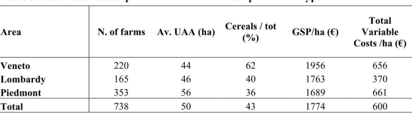
The farm sample considered in this analysis is composed of 738 farms belonging to FT1 (arable crops). The average size of each farm in the sample is 50 ha. The RICA farms in Piedmont are the largest in terms of hectares. On average the incidence of cereals on the total UAA in the sample is 43%. The average GSP per hectare is 1,774 Euros, while the total variable cost per hectare is 600 Euros (Table 3.1).

Table 3.1: Statistical description of Italian FAD' sample – Farm type 1

Area '. of farms Av. UAA (ha) Cereals / tot

(%) GSP/ha (€) Total Variable Costs /ha (€) Veneto 220 44 62 1956 656 Lombardy 165 46 40 1763 370 Piedmont 353 56 36 1689 661 Total 738 50 43 1774 600

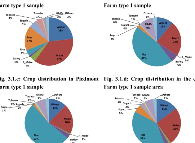
Considering the entire sample, rice covers 39% of the total land area, followed by maize with 25% and soft wheat with 15%. In Veneto maize is the main crop, while in Lombardy and Piedmont the most important crop in terms of area is rice. Another important crop is soya, that in the Veneto sample represents 17% of the entire acreage. Indeed, Veneto is specialized in producing maize and soya due to the presence of dairy and beef farms and important foodstuff industries.

(19)

Fig. 3.1.a: Crop distribution in Veneto Farm type 1 sample

Fig. 3.1.b: Crop distribution in Lombardy Farm type 1 sample

Wheat 23% Maize 37% F_Maize 4% Barley 1% Rice 4% Soya 17% Sugarb 5% Tobacco 4% Tomato 1% Alfalfa 2% Others 2% Wheat 11% Maize 23% F_Maize 0% Barley 5% Rice 46% Soya 2% Sugarb 0% Tobacco 0% Tomato 1% Alfalfa 9% Others 3%

Fig. 3.1.c: Crop distribution in Piedmont Farm type 1 sample

Fig. 3.1.d: Crop distribution in the entire Farm type 1 sample area

Wheat 12% Maize 20% F_Maize 1% Barley 3% Rice 53% Soya 1% Sugarb 0% Tobacco 0% Tomato 1% Alfalfa 7% Others 2% Wheat 15% Maize 25% F_Maize 1% Barley 3% Rice 39% Soya 5% Sugarb 2% Tobacco 1% Tomato 1% Alfalfa 6% Others 2%

All the crops depicted above are considered in the PMP model analysis and specific variable production costs are estimated for each one. As described in the previous section, the estimation is made using the information about acreage, yields, prices for each crop at farm level and the total variable cost at farm level.

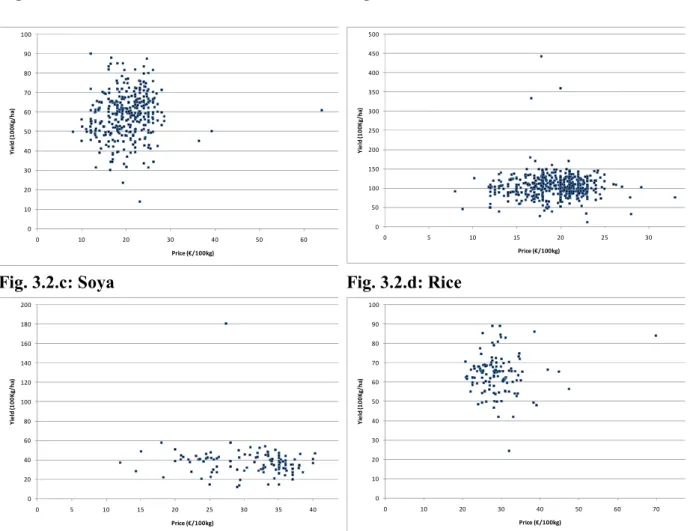
In order to achieve a good fitness of the estimation to the reality, it is important to avoid the presences of outliers, but it is also useful to utilize a homogeneous sample of farms with respect to the main variable that influences the production function and dynamics of production cost, like yields and output prices. Figure 3.2 and Table 3.2 present some descriptive information on prices and yields of four main crops included in the FADN sample.

As one can see at a first glance, the observations are less dispersed for some crops, like soft wheat and rice, while for others, like maize and soya, the dispersion is very high. The main factor that influences the observations' dispersion is the variation in yields. Indeed, for maize, the standard deviation is very high, equal to 31, which means a variation with respect the mean of 3.1 tons per hectare; while, for rice, the dispersion in yields is more restrained, 0.9 tons per hectare.

(20)

Fig. 3.2: Price and yield distribution in FT1 Sample for the Italian case study

Fig. 3.2.a: Soft wheat Fig. 3.2.b: Maize

0 10 20 30 40 50 60 70 80 90 100 0 10 20 30 40 50 60 Y ie ld ( 1 0 0 K g / h a ) Price (€/100kg) 0 50 100 150 200 250 300 350 400 450 500 0 5 10 15 20 25 30 Y ie ld ( 1 0 0 K g / h a ) Price (€/100kg)

Fig. 3.2.c: Soya Fig. 3.2.d: Rice

0 20 40 60 80 100 120 140 160 180 200 0 5 10 15 20 25 30 35 40 Y ie ld ( 1 0 0 K g / h a ) Price (€/100kg) 0 10 20 30 40 50 60 70 80 90 100 0 10 20 30 40 50 60 70 Y ie ld ( 1 0 0 K g / h a ) Price (€/100kg)

Table 3.2: Descriptives of some crops selected from FAD' sample (Lombardy, Piedmont and Veneto): price in €/100 Kg; Yields in 100 kg/ha

Crop Variable '. of Obs. MI' MAX Mean Std.

Deviation Statistic Std. Error Soft wheat Prices 335.00 8.00 64.00 20.01 0.27 5.09 Yields 335.00 13.99 90.00 58.54 0.59 11.41 Maize Prices 546.00 7.98 33.01 19.14 0.15 3.39 Yields 548.00 12.00 442.48 106.02 1.32 30.83 Soya Prices 127.00 12.00 40.26 30.85 0.53 5.98 Yields 125.00 12.19 180.77 37.74 1.42 15.88 Rice Prices 145.00 20.72 69.83 29.01 0.46 5.55 Yields 144.00 24.36 89.05 63.80 0.77 9.23

The high level of dispersion also hides the presence of outliers that can strongly influence the estimation results for some crops. For example, maize is characterized by several observations

(21)

that are out of range. Indeed, figure 3.2.b shows a cluster of points surrounded by several out of range observations. These points represent outliers that influence the capacity of the model to correctly estimate production cost and should thus be eliminated from the estimation procedure.

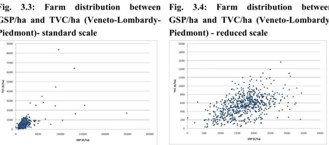
The disturbing information represented by the outliers can be appreciated at both process level and farm level. In regard to the farm information, one can see that the bad information is also present for the normalized variables concerning the gross saleable production (GSP) and farm total variable cost (TVC). Figure 3.3 shows the farms on a scatter plot considering the GSP per hectare and TVC per hectare on the axes. It is evident that some points are extremely far from the average observations and they can be considered as outliers. If we observe a detail of the same sample reducing the scale, the possibility to adopt statistical techniques aiming to detect a homogeneous set of observations is obvious.

Fig. 3.3: Farm distribution between GSP/ha and TVC/ha (Veneto-Lombardy-Piedmont)- standard scale

Fig. 3.4: Farm distribution between GSP/ha and TVC/ha (Veneto-Lombardy-Piedmont) - reduced scale

0 1000 2000 3000 4000 5000 6000 7000 8000 9000 0 5000 10000 15000 20000 25000 30000 T V C ( € / h a ) GSP (€/ha) 0 200 400 600 800 1000 1200 1400 1600 1800 2000 0 500 1000 1500 2000 2500 3000 3500 4000 T V C ( € / h a ) GSP (€/ha)

In conclusion, the strategy with respect to the outlier is to always consider all the activities present on the observed farm and to not consider in the cost estimations those farms that are outliers due to the fact that they present a single crop or many activities that are not homogeneous with respect to the characteristics of the sample. The homogeneity is evaluated by using Principal Component Analysis (PCA) and Cluster Analysis (CA). This latter is implemented using the K-mean methodology. Only the clusters with the highest number of homogeneous farms are used for the process of cost estimation by PMP model in order to guarantee sufficient numbers of observations for crops to submit to estimation.

3.2 Validation procedure

In order to validate the estimation procedure, the "estimated specific variable costs" are compared with the "observed specific variable costs" through t-test. The test allows to verify

(22)

that the two means derive from a population with the same mean (H0 : µ1 = µ2). When the probability is very low the hypothesis µ1 = µ2 is rejected.

This procedure is only possible for the Italian FADN that includes the information about specific costs per activity, while the other EU regional FADNs considered in this analysis (Belgium and Hungary) do not collect the information on production cost per activity at farm level.

3.3 Specific accounting cost estimation

In this section, we provide the estimation of variable cost per observed activity in the Italian FADN (Veneto, Lombardy and Piedmont) in different environments:

a) the entire area (the three regions together); b) each region;

c) homogeneous farm belonging the Italian FADN detected by cluster analysis.

The objective is also to show how the criteria used in the definition of the set of data becomes crucial in order to obtain a good estimation of observed variable cost.

Before discussing the analysis of the results is useful to recall that PMP allows two types of specific variable costs for each activity to be estimated: the accounting cost (c) and the marginal cost (lambda). We should be aware that these costs are estimated under economic constraints because the dual property of a profit maximization problem is used, that is implicit in the model (1)-(9), where the shadow prices associated to production activities are exactly equal to the sum of the estimated accounting cost and the estimated differential marginal

costs. The estimated accounting cost may be interpreted as the part of production shadow

price that can be explained by the accounting values, while the estimated differential marginal cost might be considered as the opportunity cost associated to each activity. The sum of the estimated accounting cost and the estimated differential marginal cost provide the exact measure of the total variable (marginal) cost associated to each activity.

The estimated differential marginal costs are defined in this work as "hidden costs", to indicate the part of estimated marginal costs that are considered by farmers in defining their production plans but which are absent from the farm accounting sheets. These are the part of marginal costs related to the specific and individual opportunity costs that each farmer has considered for deciding to introduce a given crop in the production plan. We can consider this category of costs as “pure economic cost” due to the fact that it depends on the profit maximization logic (expressed by the observed price) and on characteristics of the production function (expressed by the observed yields).

(23)

On the contrary the observed variable accounting cost registered by FADN can, in theory, contain errors due to several reasons: gathering at farm level and/or imputation. In particular farmers may wrongly specify some costs related to a production technique. One example is provided by the irrigation costs where it is difficult for farmers to properly record such costs because they are often not explicit. For these reasons the comparison of estimated variable cost with the observed marginal accounting cost can fail when some types of cost are not explicit even for farmers.

3.3.1 The estimation for Veneto, Lombardy and Piedmont as homogenous area

Table 3.3 shows the results obtained using the information on the entire sample, where the observed accounting costs are compared with the estimated accounting. Certainly the comparison is only between observed and estimated accounting cost because the hidden cost, as opportunity cost, is not collected by FADN.

Table 3.3: Comparison between observed accounting cost and specific variable cost estimated from PMP model – Veneto, Lombardy and Piedmont – Farm type 1, Year 2007 Crop Observed cost Std. Error Estimated Accounting Cost Std. Error Hidden cost Std. Error Total Marginal Cost Std. Error D_wheat 0.07575 0.00598 0.13428 0.01738 0.02680 0.00205 0.16108 0.00244 S_wheat 0.07016 0.00170 0.06602 0.00332 0.03275 0.00289 0.09878 0.00309 Maize 0.06232 0.00161 0.07439 0.00172 0.04685 0.00243 0.12124 0.00206 Barley 0.06052 0.00329 0.05130 0.00543 0.02099 0.00167 0.07229 0.00206 Rice 0.11425 0.00313 0.12368 0.00470 0.03833 0.00363 0.16201 0.00575 Sorghum 0.06466 0.01705 0.04719 0.01233 0.01949 0.00200 0.06669 0.00200 Prot_crops 0.08839 0.00904 0.08747 0.01744 0.01959 0.00323 0.10706 0.00352 Soya 0.11664 0.00590 0.09133 0.00676 0.02504 0.00333 0.11636 0.00427 Suagarbeet 0.01405 0.00050 0.01721 0.00124 0.00096 0.00015 0.01817 0.00031 Potato 0.05974 0.01268 0.12623 0.02343 0.03735 0.00908 0.16358 0.01381 Rape 0.18170 0.04158 0.11232 0.02731 0.02266 0.00238 0.13497 0.00283 Sunflower 0.11240 0.02158 0.11070 0.03307 0.02117 0.00150 0.13188 0.00197 Tobacco 0.97254 0.10625 1.03875 0.08186 0.02164 0.01118 1.06039 0.02012 Melon 0.11124 0.02712 0.12270 0.03737 0.01627 0.00230 0.13897 0.00280 Tomato 0.05094 0.01876 0.09376 0.04093 0.01844 0.00624 0.11219 0.01364 F_maize 0.02065 0.00557 0.00924 0.00240 0.00136 0.00064 0.01060 0.00084 T_grass 0.02434 0.00287 0.03165 0.00779 0.00224 0.00022 0.03389 0.00038 Alfalfa 0.01352 0.00130 0.02766 0.00316 0.00616 0.00073 0.03382 0.00088 Meadow 0.01403 0.00086 0.02986 0.00336 0.00789 0.00058 0.03775 0.00086

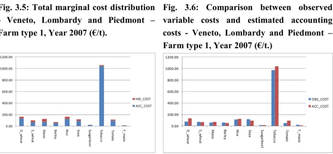
The same consideration can be appreciated observing Figure 3.5, where the estimated total variable cost is split between the accounting costs (ACC_COST) and hidden costs

(24)

(HID_COST) for some relevant activities. Tobacco is the crop with highest accounting cost, justified by the high cost of production treatment.

Fig. 3.5: Total marginal cost distribution - Veneto, Lombardy and Piedmont – Farm type 1, Year 2007 (€/t).

Fig. 3.6: Comparison between observed variable costs and estimated accounting costs - Veneto, Lombardy and Piedmont – Farm type 1, Year 2007 (€/t.)

0.00 200.00 400.00 600.00 800.00 1000.00 1200.00 D _ w h e a t S _ w h e a t M a iz e B a rle y R ic e S o y a S u a g a rb e e t T o b a c c o T o m a to F _ m a iz e HID_COST ACC_COST 0.00 200.00 400.00 600.00 800.00 1000.00 1200.00 D _ w h e a t S _ w h e a t M a iz e B a rle y R ic e S o y a S u a g a rb e e t T o b a c c o T o m a to F _ m a iz e OBS_COST ACC_COST

Figure 3.6 compares the observed accounting cost with the estimated one. For the most numerous crops, like soft wheat, maize, barley, rice and soya, the differences in absolute value remain within the range of 6% (soft wheat) to 20% (soya).

Nevertheless, the pure investigation of the differences says nothing about the statistical significance of the estimation from an inferential point of view. For this reason the t-test is introduced to verify the goodness of fit of the estimation through the comparison the mean of the estimated accounting cost with the mean of observed accounting costs.

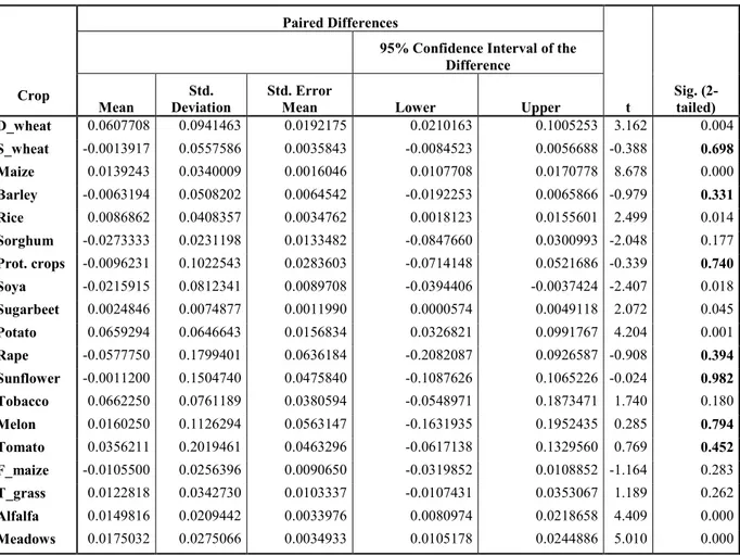
The results obtained applying Student’s t-test are presented in Table 3.4, where the most significant values are written in bold. For the entire Italian sample, the test of paired groups indicates a high significance for soft wheat, protein crops and sunflower, while for barley, rape and fodder maize the significance level is only good. For the other estimates, the null hypothesis has to be rejected for most of the crops, since the probability is lower than 1%.

(25)

Table 3.4: Student’s t-test for estimated and observed accounting costs - Veneto, Lombardy and Piedmont – Farm type 1, Year 2007.

_{Paired Differences} t Sig. (2-tailed)

95% Confidence Interval of the Difference Crop Mean Std. Deviation Std. Error

Mean Lower Upper

D_wheat 0.0607708 0.0941463 0.0192175 0.0210163 0.1005253 3.162 0.004 S_wheat -0.0013917 0.0557586 0.0035843 -0.0084523 0.0056688 -0.388 0.698 Maize 0.0139243 0.0340009 0.0016046 0.0107708 0.0170778 8.678 0.000 Barley -0.0063194 0.0508202 0.0064542 -0.0192253 0.0065866 -0.979 0.331 Rice 0.0086862 0.0408357 0.0034762 0.0018123 0.0155601 2.499 0.014 Sorghum -0.0273333 0.0231198 0.0133482 -0.0847660 0.0300993 -2.048 0.177 Prot. crops -0.0096231 0.1022543 0.0283603 -0.0714148 0.0521686 -0.339 0.740 Soya -0.0215915 0.0812341 0.0089708 -0.0394406 -0.0037424 -2.407 0.018 Sugarbeet 0.0024846 0.0074877 0.0011990 0.0000574 0.0049118 2.072 0.045 Potato 0.0659294 0.0646643 0.0156834 0.0326821 0.0991767 4.204 0.001 Rape -0.0577750 0.1799401 0.0636184 -0.2082087 0.0926587 -0.908 0.394 Sunflower -0.0011200 0.1504740 0.0475840 -0.1087626 0.1065226 -0.024 0.982 Tobacco 0.0662250 0.0761189 0.0380594 -0.0548971 0.1873471 1.740 0.180 Melon 0.0160250 0.1126294 0.0563147 -0.1631935 0.1952435 0.285 0.794 Tomato 0.0356211 0.2019461 0.0463296 -0.0617138 0.1329560 0.769 0.452 F_maize -0.0105500 0.0256396 0.0090650 -0.0319852 0.0108852 -1.164 0.283 T_grass 0.0122818 0.0342730 0.0103337 -0.0107431 0.0353067 1.189 0.262 Alfalfa 0.0149816 0.0209442 0.0033976 0.0080974 0.0218658 4.409 0.000 Meadows 0.0175032 0.0275066 0.0034933 0.0105178 0.0244886 5.010 0.000

For instance, maize that presented a difference of the estimated mean with respect the observed mean of 19%, doesn't pass the test t at a level of probability equal to zero. In other words, it is not true that the estimated mean can explain the mean of the observed costs. According to the brief statistical description of maize observations previously presented, this results may be attributable to the strong dispersion in prices and yields and to the lack of gathering specific cost related to the irrigation (that strongly influences the yields).

3.3.2 The estimation of accounting costs for each region as homogenous area

In order to assess the capability of the model to capture the territorial specificities and, thus, improve the estimates, the entire Italian sample has been stratified in three groups of farms corresponding to the three regions considered for Italy. Also in this case, the PMP model performs the estimation using all the available information presents in the sample, that consists in the activity observations for each individual farm.

3.3.2.1 The case of Veneto Region

The table 3.5 shows the estimation outputs for the Veneto region. Observing and comparing the estimated accounting cost with the observed costs is evident a strong improvement of goodness, with respect to the previous analysis. The most part of the activities, like for

(26)

example soft wheat, barley, soya and sugarbeet, the difference between the estimated and the observed accounting costs is lower than 10%. On the contrary, for some crops the divergence on the observed values remains: durum wheat estimate is completely different with respect For instance, maize, which presented a difference of the estimated mean with respect to the observed mean of 19%, doesn't pass the t-test at a level of probability equal to zero. In other words, it is not true that the estimated mean can explain the mean of the observed costs. According to the brief statistical description of maize observations given previously, this result may be attributable to the strong dispersion in prices and yields and to the lack of gathering the specific cost related to irrigation (that strongly influences yields).

3.3.2 The estimation of accounting costs for each region as a homogenous area

In order to assess the capacity of the model to capture the territorial specificities and, thus, improve the estimates, the entire Italian sample has been stratified in three groups of farms corresponding to the three regions considered. Also in this case, the PMP model performs the estimation using all the available information present in the sample, which consists of the activity observations for each individual farm.

3.3.2.1 The case of Veneto Region

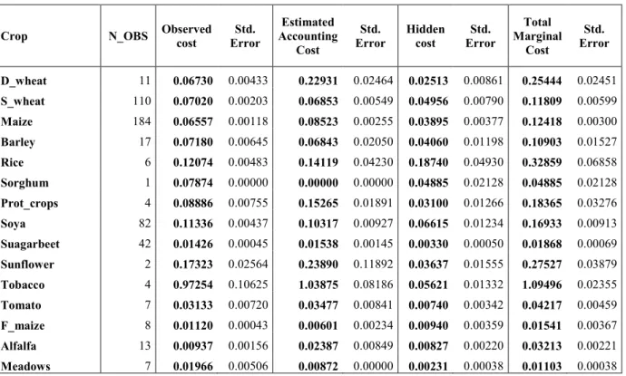
Table 3.5 shows the estimation outputs for the Veneto region. Observing and comparing the estimated accounting cost with the observed costs, there is a strong improvement with respect to the previous analysis. For most of the crops, e.g. soft wheat, barley, soya and sugarbeet, the difference between the estimated and observed accounting costs is lower than 10%. On the contrary, for some crops the divergence from the observed values remains: the durum wheat estimate is completely different from the observed data, maize also presents a divergence of 30% with respect to the observed value.

(27)

Table 3.5: Specific cost estimates obtained from PMP model - Veneto sample

Crop '_OBS Observed

cost Std. Error Estimated Accounting Cost Std. Error Hidden cost Std. Error Total Marginal Cost Std. Error D_wheat 11 0.06730 0.00433 0.22931 0.02464 0.02513 0.00861 0.25444 0.02451 S_wheat 110 0.07020 0.00203 0.06853 0.00549 0.04956 0.00790 0.11809 0.00599 Maize 184 0.06557 0.00118 0.08523 0.00255 0.03895 0.00377 0.12418 0.00300 Barley 17 0.07180 0.00645 0.06843 0.02050 0.04060 0.01198 0.10903 0.01527 Rice 6 0.12074 0.00483 0.14119 0.04230 0.18740 0.04930 0.32859 0.06858 Sorghum 1 0.07874 0.00000 0.00000 0.00000 0.04885 0.02128 0.04885 0.02128 Prot_crops 4 0.08886 0.00755 0.15265 0.01891 0.03100 0.01266 0.18365 0.03276 Soya 82 0.11336 0.00437 0.10317 0.00927 0.06615 0.01234 0.16933 0.00913 Suagarbeet 42 0.01426 0.00045 0.01538 0.00145 0.00330 0.00050 0.01868 0.00069 Sunflower 2 0.17323 0.02564 0.23890 0.11892 0.03637 0.01555 0.27527 0.03879 Tobacco 4 0.97254 0.10625 1.03875 0.08186 0.05621 0.01332 1.09496 0.02355 Tomato 7 0.03133 0.00720 0.03477 0.00841 0.00740 0.00342 0.04217 0.00459 F_maize 8 0.01120 0.00043 0.00601 0.00234 0.00940 0.00359 0.01541 0.00367 Alfalfa 13 0.00937 0.00156 0.02387 0.00849 0.00827 0.00220 0.03213 0.00221 Meadows 7 0.01966 0.00506 0.00872 0.00000 0.00231 0.00038 0.01103 0.00038

If there is a problem of number of observations for durum wheat that may have influenced the estimation, for maize the problem is different. Indeed, the number observations for this crop is very high (184), but a strong dispersion of the information on prices and, more importantly, on yields, plays an important role in procuring a distortion in the estimation results.

The analysis of the estimated accounting and hidden marginal costs (Fig. 3.7) doesn't substantially change the considerations developed for the entire sample, in the sense that the hidden cost remains a residual cost component with respect the accounting cost. As stated previously, most of the estimations are in line with the observed values, but few other estimates amplify the divergence with respect to the previous estimation (Fig. 3.8).

(28)

Fig. 3.7: Total marginal cost distribution - Veneto sample (€/t)

Fig. 3.8: Comparison between observed costs and estimated accounting costs - Veneto sample (€/t) 0.00 200.00 400.00 600.00 800.00 1000.00 1200.00 D _ w h e a t S _ w h e a t M a iz e B a rle y S o y a S u a g a rb e e t T o b a c c o T o m a to F _ m a iz e A lfa lfa HID_COST ACC_COST 0.00 200.00 400.00 600.00 800.00 1000.00 1200.00 D _ w h e a t S _ w h e a t M a iz e B a rl e y S o y a S u a g a rb e e t T o b a c c o T o m a to F _ m a iz e A lfa lfa OBS_COST ACC_COST

Table 3.6: T-test for estimated and observed accounting costs - Veneto sample

_{Paired Differences} t Sig. (2-tailed) 95% Confidence Interval of the Difference Crops Mean Std. Deviation Std. Error

D_wheat 0.1623200 0.0839499 0.0265473 0.1022659 0.2223741 6.114 0.000 S_wheat -0.0004943 0.0554849 0.0059486 -0.0123197 0.0113312 -0.083 0.934 Maize 0.0194960 0.0304049 0.0022854 0.0149858 0.0240063 8.531 0.000 Barley 0.0009273 0.0647307 0.0195170 -0.0425594 0.0444139 0.048 0.963 Rice 0.0204333 0.1101644 0.0449744 -0.0951772 0.1360438 0.454 0.669 Protein crops 0.0637500 0.0545134 0.0272567 -0.0229930 0.1504930 2.339 0.101 Soya -0.0132200 0.0873351 0.0104385 -0.0340443 0.0076043 -1.266 0.210 Sugarbeet 0.0011690 0.0086062 0.0015981 -0.0021047 0.0044426 0.731 0.471 Sunflower 0.0656500 0.2891360 0.2044500 -2.5321336 2.6634336 0.321 0.802 Tobacco 0.0662250 0.0761189 0.0380594 -0.0548971 0.1873471 1.740 0.180 Tomato 0.0019500 0.0239079 0.0097604 -0.0231398 0.0270398 0.200 0.850 F_maize -0.0044667 0.0058586 0.0033825 -0.0190203 0.0100869 -1.321 0.318 Alfalfa 0.0152000 0.0142836 0.0101000 -0.1131327 0.1435327 1.505 0.373

The t-test shows a relevant improvement in the estimation significance for most crops. For soft wheat and barley the t-test indicates a higher than 90% probability that the estimated mean is equal to the observed mean, while for sunflower and tomato the significance is over 80%. Sugarbeet, fodder maize and alfalfa also present a very good significance of the mean estimation. The worst results correspond to durum wheat and maize, for which the level of probability that the two means are equal is null. The maize results confirm those obtained for the entire sample.

3.3.2.2 The case of Lombardy region

The estimate obtained for this region, presented in Table 3.7, provides a notable increase in the estimation fitness for durum wheat, barley and soya. For durum wheat the estimated

(29)

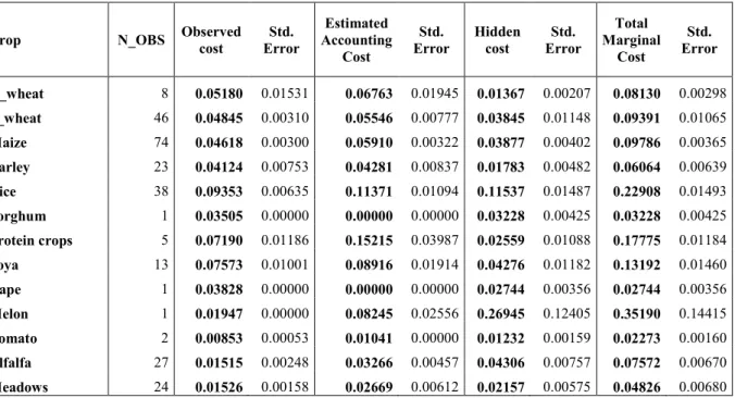
accounting cost is 30% higher than the observed cost, barley +3.8% and soya +17%. For this subset, the estimated accounting cost for soft wheat worsens with respect to Veneto and the entire sample outcomes, with a difference of +14.5% from the observed data.

Table 3.7: Specific cost estimates obtained from PMP model - Lombardy sample

Crop '_OBS Observed

cost Std. Error Estimated Accounting Cost Std. Error Hidden cost Std. Error Total Marginal Cost Std. Error D_wheat 8 0.05180 0.01531 0.06763 0.01945 0.01367 0.00207 0.08130 0.00298 S_wheat 46 0.04845 0.00310 0.05546 0.00777 0.03845 0.01148 0.09391 0.01065 Maize 74 0.04618 0.00300 0.05910 0.00322 0.03877 0.00402 0.09786 0.00365 Barley 23 0.04124 0.00753 0.04281 0.00837 0.01783 0.00482 0.06064 0.00639 Rice 38 0.09353 0.00635 0.11371 0.01094 0.11537 0.01487 0.22908 0.01493 Sorghum 1 0.03505 0.00000 0.00000 0.00000 0.03228 0.00425 0.03228 0.00425 Protein crops 5 0.07190 0.01186 0.15215 0.03987 0.02559 0.01088 0.17775 0.01184 Soya 13 0.07573 0.01001 0.08916 0.01914 0.04276 0.01182 0.13192 0.01460 Rape 1 0.03828 0.00000 0.00000 0.00000 0.02744 0.00356 0.02744 0.00356 Melon 1 0.01947 0.00000 0.08245 0.02556 0.26945 0.12405 0.35190 0.14415 Tomato 2 0.00853 0.00053 0.01041 0.00000 0.01232 0.00159 0.02273 0.00160 Alfalfa 27 0.01515 0.00248 0.03266 0.00457 0.04306 0.00757 0.07572 0.00670 Meadows 24 0.01526 0.00158 0.02669 0.00612 0.02157 0.00575 0.04826 0.00680

Figure 3.9 shows that, for Lombardy, the hidden cost represents an important component of the farmer’s decision process. In particular, this added marginal cost is important for cereals and alfalfa. Considering that the estimation deviations are all positive, this means that the outcomes overestimate the "real" accounting cost, so the production plan at regional level is strongly influenced by implicit costs that are not captured by the agricultural accounting systems.

An analysis of Figure 3.10 verifies that the estimations for cereals, soya and tomato are roughly near the target value represented by the observed accounting costs, while for protein crops and alfalfa the estimations are far from the target value. This is a simple comparison between two means that has to be verified using a statistical test.

(30)

Fig. 3.9: Total marginal cost distribution - Lombardy sample (€/t)

Fig. 3.10: Comparison between observed costs and estimated accounting costs - Lombardy sample (€/t) 0.00 50.00 100.00 150.00 200.00 250.00 D _ w h e a t S _ w h e a t M a iz e B a rle y R ic e P ro te in c ro p s S o y a T o m a to A lfa lfa M e a d o w s HID_COST ACC_COST 0.00 20.00 40.00 60.00 80.00 100.00 120.00 140.00 160.00 D _ w h e a t S _ w h e a t M a iz e B a rle y R ic e P ro te in c ro p s S o y a T o m a to A lf a lf a M e a d o w s OBS_COST ACC_COST

In order to verify that the means obtained from the individual estimated accounting costs are representative of the mean originated from the observed values, this hypothesis is submitted to the t-test. In this way, it will be possible to accept or reject the estimate obtained by implementing the PMP model. Table 3.8 presents the level of probability associated to paired groups of values (estimated and observed) for each crop. The level of significance is high for durum wheat and soft wheat, indicating that it is not possible to reject the hypothesis that the two means are different, with a probability of 66% and 63% respectively. Barley also shows a high level of significance.

Table 3.8: T-test for estimated and observed accounting costs - Lombardy sample

_{Paired Differences} t Sig. (2-tailed) 95% Confidence Interval of the Difference Crops Mean Std. Deviation Std. Error

D_wheat 0.0086167 0.0448852 0.0183243 -0.0384875 0.0557208 0.470 0.658 S_wheat 0.0044280 0.0449068 0.0089814 -0.0141086 0.0229646 0.493 0.626 Maize 0.0038746 0.0259270 0.0031675 -0.0024495 0.0101987 1.223 0.226 Barley -0.0068000 0.0339325 0.0102310 -0.0295961 0.0159961 -0.665 0.521 Rice 0.0164342 0.0495990 0.0080460 0.0001314 0.0327370 2.043 0.048 Protein crops 0.0823333 0.1128924 0.0651785 -0.1981069 0.3627736 1.263 0.334 Soya 0.0240000 0.0785200 0.0277610 -0.0416444 0.0896444 0.865 0.416 Alfalfa 0.0161696 0.0276196 0.0057591 0.0042260 0.0281132 2.808 0.010 Meadows 0.0095091 0.0273577 0.0082487 -0.0088701 0.0278882 1.153 0.276

Despite the t-test conducted for the previous samples, in this case the probability level for maize reveals a value different from zero equal to 22.6%. The significance is evidently low, but we have no reason to reject the hypothesis of equality between the two means for this crop. It is interesting to note that the significance level for maize is better where the cropping technique is almost homogenous in all the area.