Integrated experimental and numerical comparison of different approaches for planar biaxial testing of a hyperelastic material

(1)

Research Article

Integrated Experimental and Numerical

Comparison of Different Approaches for Planar

Biaxial Testing of a Hyperelastic Material

Andrea Avanzini and Davide Battini

Department of Mechanical and Industrial Engineering, University of Brescia, Via Branze 38, 25128 Brescia, Italy

Correspondence should be addressed to Andrea Avanzini; andrea.avanzini@unibs.it Received 28 October 2015; Revised 26 January 2016; Accepted 3 February 2016 Academic Editor: Jun Liu

Copyright © 2016 A. Avanzini and D. Battini. This is an open access article distributed under the Creative Commons Attribution License, which permits unrestricted use, distribution, and reproduction in any medium, provided the original work is properly cited.

Planar biaxial testing has been applied to a variety of materials to obtain relevant information for mechanical characterization and constitutive modeling in presence of complex stress states. Despite its diffusion, there is currently no standardized testing procedure or a unique specimen design of common use. Consequently, comparison of results obtained with different configurations is not always straightforward and several types of optimized shapes have been proposed. The purpose of the present work is to develop a procedure for comprehensive comparison of results of biaxial tests carried out on the same soft hyperelastic material, using different types of gripping methods and specimen shapes (i.e., cruciform and square). Five configurations were investigated experimentally using a biaxial test rig designed and built by the authors, using digital imaging techniques to track the displacements of markers apposed in selected positions on the surfaces. Then, material parameters for a suitable hyperelastic law were determined for each configuration examined, employing an inverse method which combines numerical simulations with the finite element method (FEM) and optimization algorithms. Finally, efficiency of examined biaxial configurations was assessed comparing stress reductions factor, degree and uniformity of biaxial deformation, and operative strain ranges.

1. Introduction

Biaxial testing has been employed for a long time for the study of a variety of engineering materials, including fiber reinforced composites [1, 2], plastic fabrics [3], sheet metals [4], elastomers and rubbers [5, 6], or polymers [7, 8]. This type of test has also gained considerable diffusion in the field of biomechanics and biomedical engineering, emerging as a primary technique for mechanical characterization of anisotropic, hyperelastic, and heterogeneous materials such as soft biological tissues [9–11] or biomaterials for their substitution or repair [12, 13].

The main reason that motivates planar biaxial testing is the possibility of investigating mechanical response for different combinations of stress states, providing information especially useful for the development of constitutive laws and eventually taking into account local anisotropic properties in a very effective way.

Depending on the nature of the material under investi-gation the operative range of interest, in terms of applicable loads or strains, can be quite different. Hence biaxial tests rigs (either commercial or in-house built) are often customized to serve for a specific target material [14, 15]. Consequently, there is currently no standardized testing method or a specimen configuration of universal use.

In practice two main types of specimen are employed, square or cruciform, but with several design variants and gripping techniques that can be adopted to effectively obtain a biaxial stress state over the largest possible gage area.

For square specimens load is applied along the edges, using fixtures and loading systems that allow lateral expan-sion of the specimen as the force applied along the two orthogonal axes increases. Ideally, the specimen should retain a square (or rectangular) shape with a large central region stressed biaxially. To this aim, multiple grips are distributed along the edges with low friction supports for

Volume 2016, Article ID 6014129, 12 pages http://dx.doi.org/10.1155/2016/6014129

(2)

a free transversal movement. Locally gripping may perturb this condition and special care is needed to limit frictional effects. Square specimens are usually employed also for soft biological tissues, since it may be difficult to cut them into more complex shapes. In this case, further specific issues must be considered. Different mechanisms of load transmission to the specimen may result in different degree of fiber recruitment and consequent apparent stiffness, as remarked by Waldman and Lee in [16]. The use of traditional clamping systems is prevented by the relatively small size of specimen (i.e.<20 mm) and by the risk of tissue damaging or slipping from the grips. Hence, most often the load is transferred to the specimen by means of hooks (or sutures) connected to the loading arm by suture wires and pulley systems. Special skill and fixtures for precise positioning of the hooks are needed. Such a pointwise loading may result in a less uniform stress state and premature failure of the specimen may occur due to high local stress concentrations.

Cruciform specimens are instead clamped at the end of each arm to transfer the load in the central area. In this case, the identification of an optimal shape remains a debated question, as demonstrated by the number of recent papers in which very different “optimized” specimens were proposed. Optimal cruciform specimens were investigated and analyzed by means of finite element method for stiff materials and soft materials, such as composites and various elastomers or polymeric membranes [2, 17–19]. Such “optimized” shapes may involve the introduction of different types of fillets between crossed arms, tapering of the arms, or the use of arms with slits (or even the combination of above variants). Overall, the definition of an optimal specimen shape is dictated by specific constraints imposed by the nature of material under examination as well as by the possibility of machining, cutting, or molding it into a given configuration. A further aspect that should be underlined concerns measurement of strain fields and determination of stress state actually present in the gage region of the specimen, which may represent very critical issues for biaxial testing, especially for low stiffness materials.

Different approaches to strain measurement can be found in literature. In some cases strain determination is simply based on initial reference dimensions and grips displace-ments [7], when feasible extensimetric techniques or needle extensometers [20] are used. However, for soft materials the use of noncontact methods is mandatory and video-extensometry is typically employed, tracking markers or lines apposed on the surface of the specimen during the test [9, 10]. Digital Image Correlation (DIC) techniques were also applied to analyze the whole field of biaxial deformation in the specimen [21].

A little bit more of uncertainty remains instead when considering the determination of the stress state in the central gage region of the specimen, in particular for cruciform specimens. The amount of load actually transferred to this region may differ substantially from the force measured by the load cells, depending on details of the gripping system, arms, and presence of fillets or slits. The determination by means of finite element analyses of stress correction factors is possibly the most common approach [20].

An alternative strategy, which does not require determi-nation of such correction factors, involves instead the use of inverse methods. A FE model of the test is created and by varying values of material parameters the solution of the model is iterated until some constraints imposed in terms of force or prescribed displacement are satisfied. Examples of application of this technique in presence of uniaxial and biaxial loads can be found in [22] for an estimation of parameters of Neo-Hookean and Mooney-Rivlin laws for silicon rubbers. Overall, it can be concluded that comparison of results obtained with different test rigs and different specimen shapes is not always straightforward, due to the variety of test configurations that were adopted by researchers and some inherent difficulties when interpreting results.

The purpose of the present work is to address this issue by comparing results of biaxial tests carried out on the same material but with different types of gripping methods and specimen shapes.

As anticipated, several optimized shapes were proposed but the nature of the material or the type of samples available may dictate specific constraints on the test procedure or prevent the use of an “ideal” shape as identified by means of numerical simulations. Further to this, such ideal shape could be different depending on the mechanical response expected or the strain range investigated. For this reason, rather than looking for another optimized shape, we selected a few cruciform shapes which could be readily obtained without special tools and that were previously used in different engineering fields. In particular the case of a soft material undergoing large deformation was considered, focusing on systems and specimen shapes applicable to samples of small size, obtained by means of simple cutting (or die-cutting) operations.

Then, we checked whether it was possible to determine material parameters independently of the test configuration adopted, even in presence of quite different load transmission mechanisms as well as of small mounting errors, which may be difficult to avoid when working with small compliant samples.

The final goal was to rationally compare and interpret results from different testing strategies to develop a robust and versatile testing procedure that produces comparable results independently of the test approach. This could be particularly relevant when dealing with complex materials, such as biological tissues or scaffolds used in the context of tissue engineering, in which case it may be necessary to adopt different experimental procedures depending on specific constraints imposed by the nature of materials or type of samples available.

As detailed in the next paragraphs different configura-tions were first compared experimentally, using a biaxial test rig designed and built by the authors, measuring strain by optically tracking the displacements of markers apposed on the surface in selected positions.

Then material parameters for a suitable hyperelastic law were determined for all configurations examined employing an inverse method, which combines numerical simulations and optimization algorithms.

(3)

Figure 1: Biaxial test rig.

Finally, consistency of results and efficiency of examined biaxial configurations were assessed comparing stress reduc-tions factor, biaxiality indexes, and operative strain ranges.

2. Methods

2.1. Biaxial Test Rig. Biaxial tests were carried out using a

biaxial test bench designed by the authors for testing soft materials, including soft biological tissues (see Figure 1). Briefly, the test bench consists of four independent lin-ear actuators that can be moved with a load or displace-ment/speed control. The linear motion is guaranteed by four brushed 12 V DC motors, connected to as many nylon joints that transmit the drive torque to four precision single axis actuators from Misumi (LX2001 model). Load measurements are handled by four PW6C3MR single point load cells from HBM, designed for weighing static application. The operative ranges are±200 N in terms of loads and >130 mm in terms of displacements (thus>260 mm considering an axis and not a single actuator). Load accuracy is lower than 0.05 N and displacement resolution is lower than 1𝜇m.

Different fast interchangeable gripping systems have been developed, including pulley system for tests with hooks in a trampoline-like fashion as common for soft tissues [23, 24], standard screw clamps, and wedge grips (Figure 2). Fixture and jigs for external mounting of the specimens were also designed and manufactured by rapid prototyping, both for cruciform and hooks system.

The software for the bench control and the optical meas-urements have been developed within a NI Labview real-time environment to ensure best performance.

The setup to read all the signals and to control actuators consists of an 8-slot compact RIO (cRIO-9074) module, which hosts four NI9505 modules dedicated to motors and encoders. These provide power, control the motors with a PWM (Pulse-Width-Modulation) signal, and read the output of the encoders. A single NI9237 module is dedicated to all four load cells: each load cell is connected to the module with a six-wire connection. Further modules are available to control thermocouple or heating elements (not connected for present research).

The test bench comes with an optical strain measurement based on digital tracking of the displacements of markers on the surface of the specimen. This is implemented using a Logitech C920 webcam that can record videos up to a 1920

× 1080 resolution at 30 fps, with DirectShow video output, which is very convenient for handling it with NI Labview.

The VI that operates on the webcam lets the user set opti-mal camera setting (focus, contrast, brightness, sharpness, white balance, etc.) and extracts a grayscale image for every processed frame.

The grayscale image is achieved by extracting one of the color planes describing the original image of the frame (best color plane is usually one among, red, green blue, and luminance planes). Each image is saved by Labview with the appropriate frame time so that the time information can be used for the subsequent processing and synchronizations with load cells signals.

2.2. Experimental Tests: Specimens and Procedures. This study

is focused on biaxial testing techniques for hyperelastic materials, in particular considering relatively small size of specimen. Due to the comparative nature of the investigation, tests were carried out using a rubber specimen (caoutchouc) capable of undergoing large elastic deformations but with homogeneous isotropic properties, to exclude effects directly related to specific local features of the material. As discussed in the introduction of the paper, there is currently no stan-dardized approach to biaxial testing, both for what concerns specimen and for gripping methods. Specimens shapes were therefore derived from a selection of configurations proposed in literature [18–20, 25, 26] in different fields. They were cut from a sheet of material with thickness of 0.5 mm, consider-ing different configurations as summarized in Figure 3. Four configurations had cruciform shapes that differ for presence of a fillet between intersecting arms, tapering, or inclusion of longitudinal slits to improve efficiency of load transfer. A square specimen was tested using four hooks for each side and a uniaxial tensile test was also carried out on a rectangular strip.

All the specimens were tested in displacement control moving each actuator at a speed of 0.1 mm/s.

On the surface of each specimen markers were located at specific positions of interest. For all tests, four markers were in the center of the specimen. For cruciform specimens four markers were at the intersection between the arms or in the middle of the fillets. At least one marker was located near connections between arms and central area, either at the middle or on each slit portion. The position of the hooks was also monitored. After the test, a Matlab script developed by the authors was used to process all the images saved during the test to extract the displacements of the markers. The image processing script is based on a combination of filters, edge detection, and morphing operations (dilations, erosions, filling, etc.). The script allows the user to interactively set a rectangular region of interest (ROI) and to set the number of markers to be searched. Marker centroids were calculated for every frame and their displacements were saved as a function of time into a text file for use in subsequent numerical simulation.

Note that it is also possible to calculate strain at the center of the specimen using the approach described in [27], in which central markers are treated as the nodes of an isoparametric finite element mesh.

(4)

(a) (b) (c) Figure 2: Different mounting options: hooks (a), screw clamps (b), and wedge grips (c).

20 15 40 15 15 40 40 10 15 15 50 8,50 R5 15 15 40 55 55 15 15 20 40 ₄₀ Cruciform Cruciform-fillet Square (hooks) Cruciform-slits Cruciform-tapered Uniaxial

Figure 3: Specimens (dimensions in mm).

2.3. Numerical Simulations: Constitutive Modeling and Inverse Method. The stress-strain response of the material under

examination was studied in the framework of finite strain continuum mechanics, considering constitutive models applicable to nearly incompressible hyperelastic materials. The existence of a Helmholtz free-energy or strain-energy function 𝑊 is postulated and the nearly incompressible hyperelastic behavior is treated by additive decomposition of𝑊 into the isochoric elastic part 𝑊_isoand the volumetric elastic part𝑊_vol.

This type of formulation is very often used if large elastic deformations of rubber or rubber-like material are con-cerned, because of the advantages in the numerical treatment of either incompressible or nearly incompressible properties. Several specific forms of strain-energy functions can be defined to describe the hyperelastic properties [28, 29]. Here we considered the Mooney-Rivlin (MR) form, often

employed in the description of the nonlinear behavior of isotropic rubber-like materials at moderate strain [30], as reported in

𝑊_MR= 𝑊_iso(𝐼₁, 𝐼₂) + 𝑊_vol(𝐽_el)

= 𝐶₁₀(𝐼₁− 3) + 𝐶₁₀(𝐼₂− 3) + 1₂𝑘 (𝐽_el− 1)2 (1) in which the material constants to be determined are 𝐶₁₀ and𝐶₀₁. Usually these parameters are determined by apply-ing fittapply-ing algorithms to match predicted and experimental stress-strain response. Data typically refer to a specimen gage region where strain is measured and a nominal stress can be calculated, based on some reference dimensions or assumptions. The accuracy of the fitting can eventually be checked by using the set of parameters determined for finite element simulation of an experimental test under different

(5)

conditions [31]. However, as previously mentioned, in the case of biaxial testing accurate determination of stress state in the central region can be difficult, in essence because the region of interest biaxially deformed is located in the center of the specimen, whereas the reaction forces are measured at the ends of the specimen’s arms [32]. In order to improve the correctness of stress values to be used in the fitting process, stress correction factors may then be introduced, based on FEM calculation. Ideally, the procedure for obtaining the correction factor should be repeated for any constitutive model that best suits a particular material being tested in biaxial tension [33]. Moreover, the correction factor should also be obtained for any specific specimen shape and over the strain range of interest.

An alternative approach consists in the identification of the material parameters by solving a complete boundary problem with the reaction forces as boundary condition and the displacements of selected markers in the measured area as command variable. In practice the determination of material parameters is carried out with an inverse computation, as proposed in [22, 30], by means of an adequate simulation tool capable to couple FE solution of a structural model and numerical optimization. In this study, Comsol Multiphysics was used, combining structural, nonlinear materials, PDE, and optimization modules.

In synthesis in the optimization procedure, the vector of control parameters p fl (𝐶₁₀, 𝐶₀₁) has to be modified until a close match between the experimental data and the prediction of the numerical model is achieved. To this aim, an objective function of the least squares type has to be minimized to find the optimal set of parameters:

𝑓 (p) fl 󵄩󵄩󵄩󵄩𝐷num_‖𝐷− 𝐷_exp_‖exp󵄩󵄩󵄩󵄩 󳨀→ Min (𝑓 (p)) . (2) Herein𝐷expis a vector of experimental displacements of each surface marker at each time increment.𝐷num is the vector of displacements obtained from the model, at the same time increments for the same locations of each marker, with an arbitrary set of material parameters.

It should be remarked that the choice of the optimization-based method for minimizing an objective function is still a topic of research [30] and here only the algorithms available in the optimization module of Comsol Multiphysics were considered. The present results were obtained using a Con-strained Optimization by Linear Approximation (COBYLA) algorithm [34], setting bounds and initial values of the parameters, which obviously influence convergence speed to the optimal results, based on some preliminary analysis.

For each biaxial test a FEM model was created, carrying out a stationary static analysis in which the forces measured by the load cells were introduced as boundary loads and the solution was calculated at predefined increments of time. An objective function was defined for each marker, basing on the displacements obtained with the Matlab script at the same time increments as FE solutions. It is worth noting that commonly marker displacements are applied as boundary conditions and loads as objective functions, although examples can be found in literature also for the

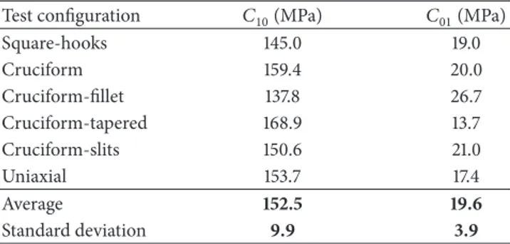
Table 1: Values of𝐶₁₀and𝐶₀₁parameters identified for different

specimen geometries.

Test configuration 𝐶₁₀(MPa) 𝐶₀₁(MPa)

Square-hooks 145.0 19.0 Cruciform 159.4 20.0 Cruciform-fillet 137.8 26.7 Cruciform-tapered 168.9 13.7 Cruciform-slits 150.6 21.0 Uniaxial 153.7 17.4 Average 152.5 19.6 Standard deviation 9.9 3.9

opposite case [32]. For the present models, we find out that with this latter approach the solution process was more efficient.

It should be noted that in the real case the distribution of transmitted force along the edges of the specimen is not known and in general, it may be different from corre-sponding numerical models. In the FE models, a uniform distribution of the load along the grips was considered, under the assumption that the area possibly perturbed by such mismatch is limited to regions close to the grips. This issue could be addressed, at least partially, by using a three-dimensional model with more details of grips/hooks interactions with specimen. This would require information about grip pressure and friction or the forces actually applied to each hook’s wire, which were not available.

Only a portion of the arms near the central region was modeled in order to reduce the computational effort for cruciform specimens. For the biaxial test with hooks, the whole specimen was considered and some markers close to the points where the hooks penetrated specimen surface were also tracked.

As biaxial alignment can be difficult when handling small samples and since the specimens were obtained by manual cutting, few small imperfections were present. Consequently, to circumvent the problem and to have more realistic simula-tions, the initial shape of the specimens and exact location of markers were directly extracted from digital image of unde-formed specimens after mounting, using CAD tools available in Solidworks. For structural analyses, triangular plane stress elements were used, taking advantage of automatic meshing algorithms to maintain an average mesh quality index of 0.95 for all models. In order to exclude mesh dependency of results, preliminary mesh convergence studies were carried out for each configuration. Depending on the complexity of geometry, the number of elements ranged from 3335 (cruciform with fillet) to 20052 (cruciform with slits).

Finally, a further set of simulations was conducted to compare the performance of different specimen geometries. In this case, average values of 𝐶₁₀ and 𝐶₀₁ (see Table 1) considering idealized geometries are reported in Figure 3.

3. Results and Discussion

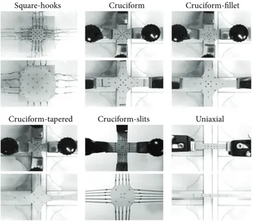
3.1. Experimental Results. In Figure 4 undeformed and

(6)

Cruciform Cruciform-fillet Square-hooks

Cruciform-slits

Cruciform-tapered Uniaxial

Figure 4: Undeformed and deformed specimens.

reported for comparison. In general, the material was capable to tolerate quite well the presence of highly localized loads (as in the case of hooks configuration) as well as of regions with geometrical discontinuities, where stress concentrations are certainly present (i.e., intersection of orthogonal arms for cruciform or tapered configuration).

For cruciform specimens, the deformed configuration was qualitatively similar with or without fillets, indicating that for this specific material the stress relief provided by the fillet is probably not necessary.

With the tapered configuration, a higher strain range was reached and the specimen changed its shape significantly. Square configuration with hooks and cruciform with slits exhibited a similar deformation of the central area, with a higher tendency to maintain a square shape of this region due to the weaker constraint imposed on transversal expansion by arms with slits and hooks, compared to full arms.

In Figure 5 load cell forces (average of four axes) are plot-ted as a function of an average Green-Lagrange strain along 𝑥- and 𝑦-axes, calculated directly from the displacements of the four central markers with the method described in [27].

The maximum forces measured by the load cells were in the range 6–10 N but the highest loads were reached only with the hooks configuration. For cruciform specimens, the tests ended because of the slippage of one of the arms from the grips. In presence of slits and hooks, the tests ended because of the failure of the specimen with fracture initiation near the apex of one of the slits or near hooks locations.

For all configurations, it was possible to reach strain levels up to about 0.7 in the central area and within this range the cruciform tapered was the one requiring the lower load (because of the reduced dimensions of central section). For all cruciform specimens, the section and area clamped in the grips were the same so they all transmitted approximately the same maximum force (about 6.35± 0.25 N). However, the corresponding strains in the central region were notably

0 2 4 6 8 10 12 0 0.5 1 1.5 2 2.5 A verag e load cell f o rc e ( N ) Average strain E Cruciform Cruciform-fillet Cruciform-tapered Cruciform-slits Square-hooks Uniax

Figure 5: Average load cell force versus average Green-Lagrange strain in central region.

different, providing a first qualitative indication that intro-duction of tapering or slits may allow the investigation, for the same load level, of more extended strain ranges.

3.2. Results of FEM Simulations with Inverse Method

3.2.1. Material Parameters and Stress-Strain Curves. As

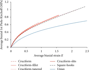
pre-viously discussed a nearly incompressible hyperelastic law of Mooney-Rivlin type was adopted as constitutive law for the material, determining material parameters𝐶₁₀ and 𝐶₀₁ by means of an inverse method applied to each configuration. Results of optimization procedure are summarized in Table 1. Overall, the range of variations of the parameters was indeed limited. The slight differences observed can be explained considering that fitting procedure is applied on different strain ranges. Some further discrepancies may arise because of the usage of test configurations that presented significant differences of initial geometries. Moreover, this method implies that the solution is sought for a large area of the specimen and not just the gage region, so that different stress states may be simultaneously present and influence the determination of parameters. On the other hand, one must also remember that FE simulations were ran on an “as mounted” condition and not on idealized model. Since some specimens were particularly difficult to cut and to set up, the fact that our results were quite consistent indicates that an inverse method may provide a robust approach allowing the correct interpretation of material parameters even in presence of small mounting errors. This is further confirmed by the stress-strain curves obtained for each configuration and reported in Figure 6. Each curve describes the biaxial stress (1st Piola-Kirchoff) against the Green-Lagrange strain, considering an averaged value between𝑋 and 𝑌 directions at the center of the specimen. As one can see, stress-strain curves are very similar, especially for strain up to 0.7. Uniaxial curve is also reported as a reference.

(7)

0 0.2 0.4 0.6 0.8 1 1.2 0 0.5 1 1.5 2 2.5 A verag e b iaxial 1s t P io la-K ir ch o ff (MP a)

Average biaxial strain E Cruciform Cruciform-fillet Cruciform-tapered Cruciform-slits Square-hooks Uniax

Figure 6: Stress-strain curves computed with finite element simu-lations. Cruciform Cruciform-fillet Square-hooks Cruciform-slits Cruciform-tapered Uniaxial 0 0.5 1 1.5 2 2.5 3 3.5 4

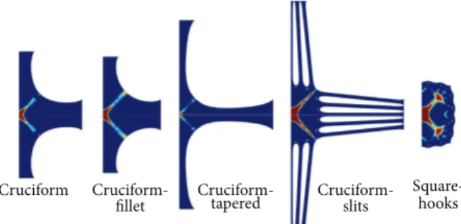
Figure 7: Contour maps of von Mises stress (MPa) superimposed on real deformed shapes of the specimens.

3.2.2. Biaxial Stress and Strain Field. Upon determination

of material parameters, the stress and strain fields were investigated by looking at the results when peak biaxial forces were reached (thus, at the end of FEA and optimization procedure).

In Figure 7 the von Mises stress contour map for each configuration is plotted and superimposed on the corre-sponding final frame acquired by the webcam. In this way it is much easier to check the correctness of the fitting process as a visual comparison can be made on the whole deformed specimen on not only the points used to define the objective functions for the optimization procedure.

In general, a very good match of predicted and exper-imental shape can be observed, confirming that the fitting process was very effective. These contour maps also provide a first evidence of the dramatic influence that test approach may have on the extension of a central area with uniform stress intensity, but this will be discussed more in detail in the next paragraph. The presence of high stress areas can as well be noticed, with predicted stress levels that, in some cases (tapered specimen), were even highly exceeding the cut-off value of 4 MPa used for the common stress scale in Figure 7.

0 0.5 1 1.5 2 2.5 3 Cruciform Cruciform-fillet Square-hooks Cruciform-slits Cruciform-tapered EYY EXX

Figure 8: Contour maps of Green-Lagrange strains𝐸_𝑋𝑋,𝐸_𝑌𝑌.

Strain fields for biaxial tests are instead reported in Figure 8, considering Green-Lagrange strains𝐸_𝑋𝑋and𝐸_𝑌𝑌 for𝑋 and 𝑌 directions.

The qualitative behavior is similar for cruciform spec-imens with and without fillet. The presence of the fillet resulted in a greater extension of a central area, with slightly lower strain levels (70% versus 80%) but relatively higher uniformity, as was also noticed in [22]. On the other hand, the introduction of the fillet does not seem to be significant for the material under investigation as the sharp edges of the no-fillet specimen become rounded as soon the specimen deforms. A fillet between arms may even limit the peak strain achievable at the center of the specimen, suggesting that its introduction should be evaluated after taking into account failure strain and resistance to damage of the material be tested.

By tapering the arm, the maximum strain level achievable increased (up to nearly 200% for tapered specimen). Again, such high levels of biaxial deformation were reached because of the capability exhibited by this specific material to tolerate extremely high strain levels, which obviously arise at the notch between intersecting arm. On one hand, this represents a positive aspect, as will be later discussed, but on the other hand, the final deformed configuration shows a quite uneven strain field, with only a restricted central area really experiencing an equibiaxial deformation. From a practical point of view, this may cause problems when considering locations for central markers.

Introducing slits into sample geometry results in high strain levels more evenly distributed over the central area and localized peaks at the apex of each slits, as also noticed in [19, 35]. This configuration, in some sense, provides a sort of approximation of a square specimen loaded along the edges, due to the weak constraint to transversal motion imposed by each single portion of the arms.

Finally, provided that the material does not fail because of high stress concentrations, high levels of biaxial strains in the central region can be reached with hooks and wires configuration. Despite the load transmission mechanism being far from uniform, the results show a quite uniform strain field in the central area where markers could be placed for the optical strain measurement.

A critical analysis of tests results also gives practical indications concerning the applicability of these test con-figurations to samples of small size. Cruciform specimens without slits were relatively easy to prepare and mount, so

(8)

0 0.5 1 1.5 2 2.5 3.5 3 4

Figure 9: Maps of von Mises stress (MPa) with underlying initial shape of the specimens (one-quarter of the nominal geometry).

experimental strain fields for𝐸_𝑋𝑋and𝐸_𝑌𝑌were symmetric, confirming a good alignment along loading axes. The config-uration with slits was more complicated to obtain and more difficult to align perfectly. Hardly noticeable differences in initial length of the slits resulted in perceivable local changes of strain distributions along the edges.

The easiest to cut is obviously a square specimen, even in presence of small size, but positioning the hooks requires special care. To facilitate our setup operations, a custom-made jig and mounting fixtures were used to ensure regular and symmetric placement along the edges. Furthermore, the loading device includes pulleys system that compensates small errors or misalignment. Despite this, hooks configura-tion exhibited the lowest degree of symmetry, mainly because of the irregular damage and elongation of the holes caused by hooks penetration. For these reasons, the comparison between different configurations is postponed to the next sec-tion, where only ideal symmetric specimens are considered. On the other hand, such experimental evidences provide a further confirmation of the usefulness of adopting an inverse method. In fact, despite differences and imperfections, this approach provided consistent values of material parameters as demonstrated by the results reported in Section 3.2.1.

3.3. Results of FEM Simulations on Ideal Shapes. As

antici-pated, FEM simulations using “as-mounted” specimen geom-etry are more realistic but, for comparison purposes, may introduce bias error due to possible slight differences between test series.

Therefore, a finite element model of the five biaxial con-figurations examined was implemented using ideal geometry and assuming average values of material parameters 𝐶₁₀ and 𝐶₀₁. Under ideal conditions, only one-quarter of the specimens was modeled taking advantage of symmetry. The same load was applied on both𝑋 and 𝑌 directions using one of the experimental load cell signals previously acquired for all the specimens.

In Figure 9 the distribution of von Mises stress is reported, using an elevation plot in which height is propor-tional to stress value. Again a cut-off value of 4 MPa is used to better appreciate stress state in the central region.

Stress maps under ideal conditions are similar to those obtained from simulations of real experiments (note that

Cruciform Cruciform-fillet Square-hooks Cruciform-slits Cruciform-tapered

Figure 10: Contour maps of biaxiality index𝑅_biax.

here the load is the same for all specimen). The presence of highly localized peak stress can be noticed for all cases, with the notable exception of the cruciform specimen with fillet. For all specimens, the stress is reasonably uniform in the central region, except for the tapered one. In fact, the tapered geometry showed a very small area with uniform stress and a steep stress gradient moving from the center of the specimen to the edges. The extension of the central area that shows a uniform biaxial deformation is fundamental to evaluate the efficiency of the specimens: the higher the ratio between the dimensions of this area and the dimensions of the specimen, the more efficient the geometry of that specimen.

For comparison purposes, one can define an index of biaxial uniformity 𝑅_biax as the ratio between the average value of strains𝐸_𝑋𝑋and𝐸_𝑌𝑌and maximum strain𝐸MAX-0,0

computed in the center point:

𝑅_biax= (𝐸𝑋𝑋+ 𝐸𝑌𝑌) /2

(𝐸_MAX)_0,0 . (3)

Contour maps of this index are shown in Figure 10, in which only areas where the absolute difference between 𝐸_𝑋𝑋 and 𝐸_𝑌𝑌is lower than 0.05 are colored (i.e., in blue area strain field is not “sufficiently” biaxial).

These maps allow a direct comparison of the efficiency of examined configurations.

We can see bigger area of uniform biaxial deformation for the square specimen with hooks and the cruciform specimen with slits.

(9)

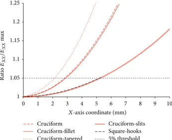
1 1.05 1.1 1.15 1.2 1.25 0 1 2 3 4 5 6 7 8 9 10 X-axis coordinate (mm) Cruciform Cruciform -fillet Cruciform -tapered Cruciform -slits Square -hooks 5% threshold Ra ti o EXX /EXX max

Figure 11: Variation of biaxiality index𝑅_biaxalong symmetry axis.

The cruciform tapered specimen presented instead a severely limited uniform area of biaxial deformation.

A quantitative evaluation of𝑅_biaxis provided in Figure 11, in which this index is plotted as a function of𝑋 coordinate along symmetry axis.

As an example, a square central area of uniform biaxial deformation can be defined for each specimen geometry by assuming a threshold value of𝑅_biax and extrapolating the corresponding𝑋 value. Specifically, assuming 𝑅_biaxthreshold value of 1.05 defines a square area with uniform biaxial deformation of about 100 mm2for the square specimen with hooks and the cruciform specimen with slits, 36 mm2 for the standard cruciform specimens (with or without fillet), and only 24 mm2for the cruciform tapered specimen. From a practical point of view, this result implies that, when choosing marker locations, particular care should be exerted not to place them outside this region of uniform biaxial deformation.

Finally, correction factors were determined by comparing the 1st Piola-Kirchoff stress computed at the center with a nominal stresses, calculated with simple formulas based on initial dimensions that can easily be measured:

Correction factor= (1st Piola-Kirchoff)

(Nominal stress) . (4) In particular, for the cruciform specimens the load cell force was divided by the section of the arms, considering a width of 15 mm. For the tapered specimen, the width considered was instead the one measured at the intersection of the arms (i.e., about 9.2 mm). For the square specimen, the side of the square inscribed by the hooks was used (15 mm).

The values of correction factors, as a function of applied strain, are summarized in Figure 12. Stress correction factors showed slight variations as strain increased.

The value of stress correction factor provides an indica-tion of the load transfer mechanism efficiency, revealing that cruciform with slits has the most uniform stress distribution

0 0.1 0.2 0.3 0.4 0.5 0.6 0.7 0.8 0.9 1 0 0.5 1 1.5 2 2.5 C o rr ec tio n fac to r

Average biaxial strain _E Cruciform

Cruciform -fillet Cruciform -tapered

Cruciform -slits Square -hooks

Figure 12: Stress correction factors.

and thus, it is possibly the most effective at transferring the load from the boundaries to the center of the specimen.

In general, computed values were comparable with those reported in literature. As an example, in [20] a reduction factor of 0.95 is used for cruciform specimen of ETFE foils with slits. In [33] a FEM based correction technique is devel-oped for both square and cruciform specimens considering anisotropy. In this case, the correction factor varied between 0.27 and 0.94 depending on shape of the specimen and material properties. Anyway, correction factors should be mainly regarded as empirical tools to improve the accuracy of simplified stress calculations.

3.4. Limitations. Mechanical characterization of hyperelastic

materials is a challenging engineering problem. Depending on the purpose of the study, different approaches can be adopted, each with different degrees of accuracy and ease of implementation. For sure in presence of materials possessing a high degree of in-homogeneity and anisotropy or under-going a general state of stress highly heterogeneous, full-field methods may capture local variations in structural response and provide a more accurate material characterization. Full-field displacement maps can be obtained with a great deal of accuracy by utilizing noncontact optical methods such as moir´e, speckle, and holography. Measured displacements are then compared with numerical predictions provided by finite element. Among others, an example of application of such methods is provided in [36], in which case moir´e techniques and advanced optimization algorithms were used to identify constitutive behavior and material parameters of hyperelastic membranes, including bovine pericardium patches. In [32] silicone rubber was characterized by combining the use of DIC and optimization algorithms. A different approach involves the use of the virtual fields method (VFM). The base of the method and references about its applications to a variety of materials can be found in [37]. More specifically the feasibility of its application for low-density hyperelastic foams has been investigated in [38]. Recently the use of such

(10)

technique has been extended to the characterization of visco-hyper-pseudo elasticity in fluoro-silicon rubbers [39]. In [40] investigations with VFM on thermomechanical response of three-branch were instead reported.

On the other hand, possibly because of its straightforward implementation, marker tracking technique is still widely employed, especially for soft biological tissues. Most often only the displacements of a set of markers in the central gage region are monitored, but noticeably in [41] the use of several randomized markers tracked with a DIC system has been reported. Such information is then used for the construction of stress-strain curves to be fitted, under some simplifying assumptions, with appropriate constitutive laws.

Recently a hybrid procedure based on inverse method, similar to the one adopted in the present work, was adopted to characterize porcine aortic tissue [42]. In consideration of comparative nature of the present study, with different geometries and experimental set up, we opted for this latter approach, providing a good balance between accuracy and ease of implementation. Since the material under exami-nation was homogeneous and isotropic, this approach was deemed to be sufficiently accurate. Of course, it might be very useful to integrate the present analysis with a full-field measurement technique, especially for specimens exhibiting local regions with high stress gradients. This is planned as a future development.

A further relevant aspect is that stress distribution and concentration depend on the material behavior. In the present comparative study, only one class of materials was considered and this partially reduces the generality of the results. In par-ticular, it should be remarked that soft biological tissues may exhibit far more complicated mechanical behaviors. In order to extend the interpretation of results to this type of materials, further issues have to be considered, such as the influence of boundary conditions on load transmission mechanisms and fiber recruitment, or the higher mathematical complexity of procedures for the determination of material parameters.

The influence of varying the degree of anisotropy (i.e., fiber orientation) for square and cruciform geometries was investigated by means of finite element simulations in [33]. Stress concentrations were greater for the square geometry than the cruciform geometry and fiber alignment parallel to the loading axes increased the load being transferred to the central region of interest. The application of a correction factor to experimental biaxial results was also suggested to obtain more accurate representation of the mechanical response of fibrous soft tissue. However, to the best of authors’ knowledge, an experimental comparison considering hyperelastic-anisotropic behavior has not yet been reported in literature. This would imply availability of tissue (engineered) samples with different geometries, in which the degree of anisotropy (i.e., the fiber architecture) is manageable and perfectly known in advance. Furthermore, constitutive behavior of anisotropic materials identified via hybrid procedures should be validated by carrying out other independent tests. Considering the comparative nature of the present study, at this stage such kind of investigation was beyond our scope, but it certainly represents an important field of research for the future.

4. Conclusions

Different configurations for planar biaxial testing of a hyper-elastic material were compared both experimentally and with FEM simulations, using an inverse method to determine material parameters for a Mooney-Rivlin hyperelastic law. The main conclusions are as follows:

(1) Biaxial configurations chosen between those used (or proposed) for testing small samples of highly deformable materials may present substantial differ-ences in terms of stress and strain distributions, con-firming that interpretation of results can be difficult and care is needed when comparing.

(2) The inverse method proved to be a useful approach to compare different biaxial testing methodologies, overcoming the problem of determining real stress states by correction factors to improve fitting accu-racy. Similar values of materials parameters were in fact obtained in presence of completely different specimen geometries.

(3) When a cruciform specimen is used, arms with slits may substantially improve efficiency of load transfer to the central region and degree of biaxial uniformity. With tapered arms the central region can be subjected to high stress and strain levels, but a significant decay of uniformity is present and this may impair strain measurements. Use of fillets reduces stress concentration and loading efficiency as well.

(4) Square specimen tested with hooks may provide a viable way for biaxial testing but require special care for sample manipulation and hooks application, due to high sensitivity even to small mounting errors. (5) Some types of specimens and loading systems could

lead to stress concentrations that may, or may not, be tolerated depending on material properties. Different materials may impose different constraints in terms of machinability of complex shapes of the specimen. Optimized shapes should then be evaluated for each specific material investigated with biaxial testing. (6) Stress correction factors can help in improving

accu-racy of stress calculation, but when dealing with highly nonlinear materials they should be determined with some understanding of the constitutive law to be used and of the strain range of interest.

In conclusion, a relevant contribution of the present study is that integrating the use of inverse method with markers’ measurements can actually lead to the determination of very similar sets of material parameters (and corresponding stress-strain curve), even if very different experimental configura-tions are adopted. Such evidence is particularly relevant since, while keeping a traditional experimental setup, it overcomes the problem of introducing correction factors “configuration dependent” for stress determination, allowing comparison of different efficiency of specimens shapes and loading modes. In this respect, it has to be underlined that differently to most of published literature such comparison is not limited

(11)

to a numerical investigation but relies on experimental observations. We not only compared numerically on the same material cruciform and square shape but also actually imple-mented two different gripping systems, with grips and hooks and considering realistic dimensions, with size comparable to those of biological tissue samples. The direct comparison of cruciform and square specimen is a novel contribution that could be particularly relevant for researchers dealing with complex materials, such as biological tissues or scaffolds used in the context of tissue engineering, in which case it may be necessary to adopt different experimental procedures.

Conflict of Interests

The authors declare that there is no conflict of interests regarding the publication of this paper.

Acknowledgment

The authors would like to acknowledge that the work was supported in part by Bio@BeSt grant from DIMI-UniBS for the design and construction of the biaxial test rig.

References

[1] D. A. Arellano Escarpita, D. Cardenas, H. Elizalde, R. Ramirez, and O. Probst, “Biaxial tensile strength characterization of textile composite materials,” in Composites and Their Properties, N. Hu, Ed., chapter 5, pp. 83–106, IntechOpen, doi, 2012. [2] A. Smits, D. Van Hemelrijck, T. P. Philippidis, and A. Cardon,

“Design of a cruciform specimen for biaxial testing of fibre reinforced composite laminates,” Composites Science and

Tech-nology, vol. 66, no. 7-8, pp. 964–975, 2006.

[3] C. Galliot and R. H. Luchsinger, “A simple model describing the non-linear biaxial tensile behaviour of PVC-coated polyester fabrics for use in finite element analysis,” Composite Structures, vol. 90, no. 4, pp. 438–447, 2009.

[4] A. Hannon and P. Tiernan, “A review of planar biaxial tensile test systems for sheet metal,” Journal of Materials Processing

Technology, vol. 198, no. 1–3, pp. 1–13, 2008.

[5] R. J. Arenz, R. F. Landel, and K. Tsuge, “Miniature load-cell instrumentation for finite-deformation biaxial testing of elastomers,” Experimental Mechanics, vol. 15, no. 3, pp. 114–120, 1975.

[6] D. J. Charlton, J. Yang, and K. K. Teh, “Review of methods to characterize rubber elastic behavior for use in finite element analysis,” Rubber Chemistry and Technology, vol. 67, no. 3, pp. 481–503, 1994.

[7] S. Becker, C. Combeaud, F. Fournier, J. Rodriguez, and N. Billon, “Biaxial tension on polymer in thermoforming range,” EPJ Web

of Conferences, vol. 6, article 25003, 8 pages, 2010.

[8] G. H. Menary, C. W. Tan, E. M. A. Harkin-Jones, C. G. Arm-strong, and P. J. Martin, “Biaxial deformation and experimental study of PET at conditions applicable to stretch blow molding,”

Polymer Engineering and Science, vol. 52, no. 3, pp. 671–688,

2012.

[9] M. S. Sacks, “Biaxial mechanical evaluation of planar biological materials,” Journal of Elasticity, vol. 61, no. 1–3, pp. 199–246, 2000.

[10] M. Zem´anek, J. Burˇsa, and M. Dˇet´ak, “Biaxial tension tests with soft tissues of arterial wall,” Engineering Mechanics, vol. 16, no. 1, pp. 3–11, 2009.

[11] A. Eilaghi, J. G. Flanagan, I. Tertinegg, C. A. Simmons, G. W. Brodland, and C. R. Ethier, “Biaxial mechanical testing of human sclera,” Journal of Biomechanics, vol. 43, no. 9, pp. 1696– 1701, 2010.

[12] A. V. Kamenskiy, I. I. Pipinos, J. N. MacTaggart, S. A. Jaffar Kazmi, and Y. A. Dzenis, “Comparative analysis of the biaxial mechanical behavior of carotid wall tissue and biological and synthetic materials used for carotid patch angioplasty,” Journal

of Biomechanical Engineering, vol. 133, no. 11, Article ID 111008,

2011.

[13] B. J. Bell, E. Nauman, and S. L. Voytik-Harbin, “Multiscale strain analysis of tissue equivalents using a custom-designed biaxial testing device,” Biophysical Journal, vol. 102, no. 6, pp. 1303–1312, 2012.

[14] A. Makinde, L. Thibodeau, and K. W. Neale, “Development of an apparatus for biaxial testing using cruciform specimens,”

Experimental Mechanics, vol. 32, no. 2, pp. 138–144, 1992.

[15] J. P. Boehler, S. Demmerle, and S. Koss, “A new direct biax-ial testing machine for anisotropic materbiax-ials,” Experimental

Mechanics, vol. 34, no. 1, pp. 1–9, 1994.

[16] S. D. Waldman and J. M. Lee, “Boundary conditions during biaxial testing of planar connective tissues. Part 1: dynamic behavior,” Journal of Materials Science: Materials in Medicine, vol. 13, no. 10, pp. 933–938, 2002.

[17] A. S. Torres and A. K. Maji, “The development of a modified bi-axial composite test specimen,” Journal of Composite Materials, vol. 47, no. 19, pp. 2385–2398, 2013.

[18] P. Tiernan and A. Hannon, “Design optimisation of biaxial ten-sile test specimen using finite element analysis,” International

Journal of Material Forming, vol. 7, no. 1, pp. 117–123, 2014.

[19] X. Zhao, Z. C. Berwick, J. F. Krieger, H. Chen, S. Chambers, and G. S. Kassab, “Novel design of cruciform specimens for planar biaxial testing of soft materials,” Experimental Mechanics, vol. 54, no. 3, pp. 343–356, 2014.

[20] C. Galliot and R. H. Luchsinger, “Uniaxial and biaxial mechan-ical properties of ETFE foils,” Polymer Testing, vol. 30, no. 4, pp. 356–365, 2011.

[21] L. Chevalier and Y. Marco, “Tools for multiaxial validation of behavior laws chosen for modeling hyper-elasticity of rubber-like materials,” Polymer Engineering and Science, vol. 42, no. 2, pp. 280–298, 2002.

[22] H. Seibert, T. Scheffer, and S. Diebels, “Biaxial testing of elastomers—experimental setup, measurement and experimen-tal optimisation of specimen’s shape,” Technische Mechanik, vol. 34, no. 2, pp. 72–89, 2014.

[23] A. N. Azadani, S. Chitsaz, P. B. Matthews et al., “Comparison of mechanical properties of human ascending aorta and aortic sinuses,” Annals of Thoracic Surgery, vol. 93, no. 1, pp. 87–94, 2012.

[24] T. Pham and W. Sun, “Material properties of aged human mitral valve leaflets,” Journal of Biomedical Materials Research Part A, vol. 102, no. 8, pp. 2692–2703, 2014.

[25] C.-S. Jhun, M. C. Evans, V. H. Barocas, and R. T. Tranquillo, “Planar biaxial mechanical behavior of bioartificial tissues pos-sessing prescribed fiber alignment,” Journal of Biomechanical

Engineering, vol. 131, no. 8, Article ID 081006, 8 pages, 2009.

[26] R. Raghupathy, C. Witzenburg, S. P. Lake, E. A. Sander, and V. H. Barocas, “Identification of regional mechanical anisotropy in soft tissue analogs,” Journal of Biomechanical Engineering, vol. 133, no. 9, Article ID 091011, 2011.

(12)

[27] A. Hoffmann and P. Grigg, “A method for measuring strains in soft tissue,” Journal of Biomechanics, vol. 17, no. 10, pp. 795–800, 1984.

[28] Y. Bitoh, N. Akuzawa, K. Urayama, and T. Takigawa, “Strain energy function of swollen polybutadiene elastomers studied by general biaxial strain testing,” Journal of Polymer Science, Part B:

Polymer Physics, vol. 48, no. 6, pp. 721–728, 2010.

[29] F. Q. Pancheri and L. Dorfmann, “Strain-controlled biaxial tension of natural rubber: new experimental data,” Rubber

Chemistry and Technology, vol. 87, no. 1, pp. 120–138, 2014.

[30] Z. Chen, T. Scheffer, H. Seibert, and S. Diebels, “Macroinden-tation of a soft polymer: identification of hyperelasticity and validation by uni/biaxial tensile tests,” Mechanics of Materials, vol. 64, pp. 111–127, 2013.

[31] M. Fujikawa, N. Maeda, J. Yamabe, Y. Kodama, and M. Koishi, “Precise measurement technique of stress-strain relationship for rubber using in-plane biaxial tensile tester,” in Constitutive

Model for Rubber, B. Marvalova and I. Petrikova, Eds., Taylor &

Francis Group, London, UK, 2015.

[32] M. Johlitz and S. Diebels, “Characterisation of a polymer using biaxial tension tests. Part I: hyperelasticity,” Archive of Applied

Mechanics, vol. 81, no. 10, pp. 1333–1349, 2011.

[33] N. T. Jacobs, D. H. Cortes, E. J. Vresilovic, and D. M. Elliott, “Biaxial tension of fibrous tissue: using finite element methods to address experimental challenges arising from boundary con-ditions and anisotropy,” Journal of Biomechanical Engineering, vol. 135, no. 2, Article ID 021004, 10 pages, 2013.

[34] “Comsol multiphysics 5.1—optimization module user’s guide,” in The Optimization Solvers, A. B. Comsol Multiphysics, Ed., chapter 5, pp. 51–88, 2015.

[35] K. A. Lyadova, V. V. Shadrin, L. V. Kovtanyuk, and A. S. Usti-nova, “Shape optimization of a biaxially loaded specimen,” in

Proceedings of the XLI International Summer School-Conference “Advanced Problems in Mechanics” (APM ’13), pp. 360–367,

Saint Petersburg, Russia, July 2013.

[36] E. Cosola, K. Genovese, L. Lamberti, and C. Pappalettere, “A general framework for identification of hyper-elastic mem-branes with moir´e techniques and multi-point simulated annealing,” International Journal of Solids and Structures, vol. 45, no. 24, pp. 6074–6099, 2008.

[37] M. Gr`ediac and F. Pierron, “Identifying constitutive parame-ters from heterogeneous strain fields using the virtual fields method,” Procedia IUTAM, vol. 4, pp. 48–53, 2012.

[38] F. Pierron and B. Guo, “Identification of the mechanical behaviour of low density hyperelastic polymeric foams from full-field measurements,” Journal of Physics: Conference Series, vol. 181, no. 1, Article ID 012044, 2009.

[39] M. Sasso, G. Chiappini, M. Rossi, L. Cortese, and E. Mancini, “Visco-Hyper-Pseudo-Elastic characterization of a Fluoro-Silicone rubber,” Experimental Mechanics, vol. 54, no. 3, pp. 315– 328, 2014.

[40] E. Toussaint, X. Balandraud, J. B. Le Cam, and M. Gr`ediac, “Application of full-field measurements to analyse the thermo-mechanical response of a three-branch rubber specimen,” in

Imaging methods for Novel Materials and Challenging Appli-cations: Imaging Methods for Novel Materials and Challenging Applications, Volume 3, H. Jin, C. Sciammarella, C. Furlong,

and S. Yoshida, Eds., Conference Proceedings of the Society for Experimental Mechanics Series, chapter 37, pp. 263–268, 2013. [41] J. A. Pe˜na, M. A. Mart´ınez, and E. Pe˜na, “Layer-specific residual

deformations and uniaxial and biaxial mechanical properties of thoracic porcine aorta,” Journal of the Mechanical Behavior of

Biomedical Materials, vol. 50, pp. 55–69, 2015.

[42] J. O. V. Delgadillo, S. Delorme, F. Thibault, R. DiRaddo, and S. G. Hatzikiriakos, “Large deformation characterization of porcine thoracic aortas: inverse modeling fitting of uniaxial and biaxial tests,” Journal of Biomedical Science and Engineering, vol. 8, no. 10, pp. 717–732, 2015.

(13)

Submit your manuscripts at

http://www.hindawi.com

Scientifica

Hindawi Publishing Corporation

http://www.hindawi.com Volume 2014

http://www.hindawi.com Volume 2014 Hindawi Publishing Corporation

Ceramics

Journal of

Nanoparticles

Journal of Hindawi Publishing Corporation

International Journal of

Biomaterials

Nanoscience

Journal of

Textiles

Crystallography

The Scientific

World Journal

Coatings

Journal of

Advances in

Materials Science and Engineering

Metallurgy

Journal of

BioMed

Research International

Materials

N

a

no

ma

te

ria

ls

Hindawi Publishing Corporation

http://www.hindawi.com Volume 2014

Journal of