Universit`
a degli Studi Roma Tre
Dottorato di Ricerca in FisicaXXII Ciclo (2006-2009)
Ab initio investigation of the structural and
electronic properties of TiO
2nanostructures.
Thesis for Doctor of Philosophy degreesubmitted by Amilcare Iacomino
Supervisors:
Chia.mo Prof. Florestano Evangelisti
Chia.mo Prof. Domenico Ninno
Dr. Giovanni Cantele
Coordinator:
Contents
Introduction 3
1 Theoretical framework of first-principles calculations 9
1.1 The quantum many-body problem . . . 10
1.2 Density Functional Theory . . . 12
1.2.1 The electron density as fundamental variable . . . 13
1.2.2 The Kohn-Sham equations . . . 15
1.2.3 Approximations for the exchange-correlation energy . . . 17
1.3 Basis representation and pseudopotentials . . . 18
1.3.1 The pseudopotentials technique . . . 20
1.4 Structural optimization . . . 22
1.5 Modeling low dimensional systems . . . 24
2 An overview of experimental techniques and measurements 27 2.1 Synthesis of TiO2 nanostructures . . . 27
2.2 Structural determinations . . . 31
2.2.1 X-ray electron diffraction on powders . . . 31
2.2.2 Extended X-ray absorption fine structure . . . 33
2.2.3 Transmission electron microscopy . . . 36
2.2.4 Infrared spectroscopy . . . 38
2.3 Electronic determinations . . . 40
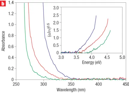
2.3.1 Ultraviolet-visible absorption measurements . . . 41
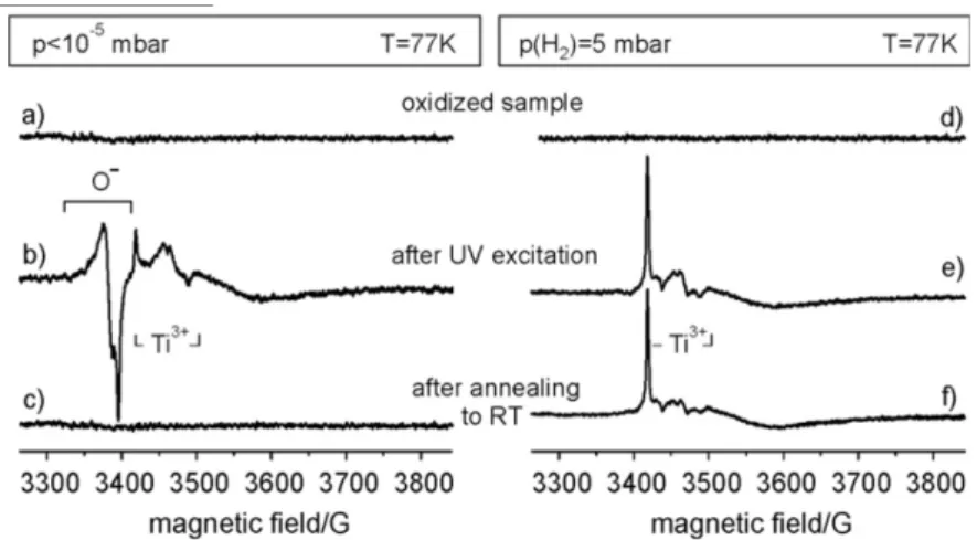
2.3.2 Electron paramagnetic spectroscopy . . . 43
3 TiO2 0D nanocrystals 47
3.1 Methodology . . . 50
3.2 Results and discussion: structure . . . 52
3.2.1 NCs volume . . . 53
3.2.2 The bond lengths in the octahedron and distances of atomic pairs . . . 54
3.3 Results and discussion: electronic properties . . . 57
3.3.1 From crystal to NC . . . 57
3.3.2 Effects of the surface coverage . . . 60
3.3.3 Band gap . . . 63 3.3.4 HOMO-LUMO states . . . 65 3.4 Formation energies . . . 68 3.5 Conclusions . . . 70 4 TiO2 1D nanowires 73 4.1 Methodology . . . 76 4.1.1 Computational details . . . 76 4.1.2 NWs definition . . . 77
4.2 Results and discussion: structure . . . 80
4.2.1 Section area variations . . . 81
4.2.2 Variations of the atomic distances . . . 83
4.3 Results and discussion: electronic properties . . . 85
4.3.1 Effects of the size reduction . . . 85
4.3.2 Bands line-up . . . 90
4.3.3 Pathways of reactions at the surface of the NWs . . . 93
4.3.4 Hydrogen sensing ability of the NWs . . . 96
4.4 Relative stability analysis . . . 98
4.5 Conclusions . . . 101
Conclusions 105
Introduction
Nanoscience constitutes a rapidly evolving branch of the modern scientific research due to the contemporary convergence of different interests. Firstly, the technological capabilities are nowadays at pace to constantly carry out new and unprecedented nanobased devices, nanoscaled assemblies of heterogeneous materials, and stand-alone nanostructures in a variety of arrangements. A the same time, state-of-the-art measurement techniques progressively succeed in revealing several properties of the nanomaterials thus drawing a general portrait of their features. Secondly, the evi-dence of the new and peculiar properties that materials show at the nanoscale with respect to their macroscopic counterparts opens up fascinating expectations to em-ploy more and more optimized nanodevices in many fields of social and commercial relevance. Thirdly, the current theoretical research is developing practical tools to investigate reliable models of feasible nanostructures, thus standing as an effective asset to integrate, support, and organize the experimental bunch of results.
In this thesis we focused on the study of low dimensional titanium dioxide (TiO2), which is worldwide acknowledged as an outstanding example of the deep impact that nanoscale manipulation can induce into the daily life and society. In fact, TiO2 is a cheap and biocompatible semiconductor, well known for its striking photocatalytic performances in many reactions. The possibility to synthesize TiO2 based materials in the nanometer scale paves the way to design new devices with enhanced efficiencies for, e.g. solar energy conversion of light (dye synthesized solar cells or DSSCs) [1], water splitting process for large scale hydrogen production (sustainable fuel) [2], selective inactivation of diseased tissues (decrement of side effects) [3, 4], manageable employment of self-cleaning coatings (art protection and ambient sterilization) [5, 6], efficient photodegradation of organic pollutants in waste water and air [7]. The list
is far to be completed since new applications show up with the progress in research [8, 9, 10, 11]. All these achievements rely on the efficient control and tuning of the peculiar properties emerging at nanoscale to ultimately enhance specific processes of interest.
Within the above mentioned general framework, this thesis is meant to contribute to a comprehensive study of the fundamental properties of TiO2 zero-dimensional nanocrystals (0D NCs) and one-dimensional nanowires (1D NWs), through the anal-ysis of the connection between our theoretical results and experimental findings available in the literature. We have performed first-principles calculations on both 0D NCs and 1D NWs based on the density functional theory (DFT), which is a powerful tool to obtain both structural and electronic informations from an ab-initio approach. Some properties of TiO2 nanomaterials are still debated, since their unanimous understanding is subordinate to the ability to isolate and identify single processes in a variety of phenomena taking place at the same time, which is obviously a challenging task for the modern probing instruments and technology. Hence, one goal of this thesis is to shed light on some controversial properties of TiO2 nanostructures. Furthermore, the second goal of this thesis is to outline a the-oretical background of knowledge, readily available for the experimental designing of new TiO2 nanomaterials and devices.
The first class of TiO2 systems that we will consider is constituted by 0D NCs. There are many open questions about nanostructured TiO2, some of which will be addressed in this thesis. The reduction of sample size produces an unavoidable variation of the structural arrangement. Lattice parameters of the anatase crystal phase have been observed to expand in some cases or to contract in others [12], while the rutile phase and other metal oxides show a linear expansion on decreasing the particle size. The bulk coordination of Ti is preserved in internal NC cells but the surface truncation produces undercoordination, dangling bonds and surface tension whose effect is a local disorder [14]. Some experimental works have observed in the smallest nanosamples (< 5 nm) the variation of bond lengths and coordination numbers upon decreasing the NC size [14, 15, 16, 17, 18]. This suggests an influence of the surface on the overall structure. Reactive compounds in solution can change the NC morphology as proved by the restoring of the octahedral coordination for the surface Ti atoms after adsorption of radicals [15, 19]. Modern instruments face
a challenging task when dealing with the dislocation of atoms at the surface of nanoparticles, since usual methods, like XRD and LEED, are unable to handle such size confined samples. On the other hand, our DFT approach have already proved to give reliable results in describing TiO2 atomic arrangements and dislocations [20], thus we will address the structural deformations by total energy optimizations of our model systems. We will show the influence that surface termination has in determining the overall crystallinity of the NCs and its effects on the local order of the bonds geometry, thus suggesting an interpretation of the experimental findings. The anatase TiO2 crystal is an indirect semiconductor. On a theoretical general ground, a decrease of the dimensions down to the nanometer scale makes the electron mean free path comparable with system size; thus, one would expect a quantum size effect to be measurable through the band gap blue shift. This shift is not always detectable in nanostructured TiO2: (i) some authors [21, 22, 23] observed the bulk gap for sample diameters down to 1.5 nm; (ii) others [10, 24, 25] measured a blue shift already in the range 5− 10 nm; (iii) red shifts are also observed and mainly ascribed to the presence of surface oxygen vacancies, to adsorbates or dopants producing electronic states in the forbidden region [10]. The nature of the first allowed transition is still under debate as well, since a direct radiative decay blue shift of the band gap is advised [11, 22, 26]. We will show through the analysis of the electronic properties, that the structural arrangement and the surface coverage can deeply influence the overall electronic structure, thus hindering or highlighting the effects of size confinement.
TiO2 is the best candidate for photovoltaic solar cell conversion of light and for water splitting with consequent hydrogen production on a large scale [1, 27]. These ambitious goals need a deep understanding of the interaction of TiO2 with water and its constituents. The presence of a large hydration sphere surrounding TiO2 nanoparticles is usually detected [28] and may play a fundamental role in photo-catalysis. This hydration sphere is built up of different and non equivalent bonds between water and the TiO2 surface, forming a multilayered wet sphere. On the other hand, early works directly focused on the TiO2-H surface interaction and dop-ing of NCs have been reported very recently [29, 30]. Hence we decided to cover our bare systems with simple adsorbates (H2 and H2O), modeling surface configurations in presence of hydrogens and hydration. It is evident that the very numerous
experi-mental data on TiO2 NCs produced a large variety of, often conflicting, results. The lack of a satisfactory and organic comprehension of many of the measured properties can certainly be ascribed to the TiO2 own nature - very high reactivity toward the external environment, ability to sustain complex surface chemistry, O vacancies, etc. Our DFT approach is functional to consider single representative configurations of the NCs, thus allowing a direct characterization of the effects induced by one phe-nomenon at a time (i.e. oxygen desorption, hydrogen adsorption, etc.), accordingly to which we will show the trends of the overall properties.
The second class of TiO2 systems that we will consider is constituted by 1D NWs. Actually, TiO2 0D NCs and 1D NWs share the same benefits from having larger surface area, more active sites, and quantum confinement related proper-ties which eventually lift the rates of their activity [31, 32, 33]. 1D nanotubes, nanorods, and NWs are sometimes polycrystalline assemblies of NCs [34], hence the elementary physical properties can overlap. The main feature that can distinguish TiO2 1D nanostructures from their 0D counterpart is a better ability to transport (photo)generated charges away from possible (recombination) reaction sites, thus re-vealing the heavy attention they are receiving for applications in photovoltaic cells, sensors, electrodes, and optoelectronics [35].
Our theoretical investigation may fill the gap through the atomistic modeling of TiO2 nanostructures, by proposing the fundamental understanding of the physical properties behind the observed mechanisms at the nanoscale. Despite the example of the well characterized 1D nanomaterials like silicon and carbon, a very scarce literature is directly focused on the study of TiO2 1D nanostructures up to now [36, 37, 38, 39]. The aim of this thesis is to investigate the dependence of the structural, electronic, and stability properties of anatase TiO2 NWs as functions of the surface coverage, of the diameter size, and of the morphology, within the framework of first-principles DFT calculations. We will define two types of NWs with different growth direction and exposed surfaces to account for the morphological dependent properties. For a given type of NW we will consider four diameter sizes to address the trends of the properties with the dimension and, at last, we will cover the surface of the NWs as in the case of 0D NCs to study the influence of adsorbates on the overall properties of the NWs. We will study some issues that are in common with 0D NCs, that is the structural deformations at the nanoscale, the expected size confinement
through the blue shift of the band gap, and the effects of the interaction with water derived adsorbates. Moreover, we will address specific aspects of 1D NWs that are still under investigation due to the actuality of the research in this field. The band gap blue shift due to the scaling of the dimension down to the nanometer range could contribute to improve the charge transfer between the NW and the reactive species if a proper line-up of the valence band maximum for holes or conduction band minimum for electrons, with respect to the redox couple potentials, is satisfied. We will elucidate the effect of the size, of the surface configuration, and of the morphology on the NW ability to photocatalyze reactions through the calculation of a unique line-up of the bands energies.
Another issue discussed in this thesis is related with the efficiency of TiO2 NWs to support photocatalytic reactions and the charge transport of photoelectrons to external circuits (for photosensing and solar cells applications). Both mechanisms are linked to the nature of the charge density distribution of the states involved in the transfer of charges. In fact the probability of the charge transfer increases with the overlap between the donor/acceptor wave functions of the NW and the reactant. To support the transport of photoelectrons throughout the external circuit it is also necessary that conduction band channels flow inside the NW to lengthen the lifetime of charges by avoiding recombination centers, i.e. structural distorsions, defects, and charge traps which are mainly located at the surface. We will address this issue through calculations of the density of states and of the charge density distribution of the states in the NWs.
The last important application under investigation deals with the possibility to employ TiO2 NWs as hydrogen sensors. Experiments reveal that TiO2 nan-otubes [40, 41] and mesowires [42] show an increase of the conductance upon expo-sure to hydrogen gas, which can be of some orders of magnitude [43] and can lead to the highest variation of the electrical properties of a material, to any gas, ever shown [44]. The main mechanism is ascribed to the adsorption of the dissociated hydrogen molecules at the surface due to the high electrical variation, velocity, and reversibility of the sensing process [45]. We will study the effect of the hydrogen surface coverage on the electronic structure of our TiO2 NWs to identify and predict their ability to detect hydrogen gas. We will also relate our results to the size and the morphology of the NWs, thus giving useful informations to take into account
when designing new TiO2 nanodevices.
The thesis is organized as follows. In chapter 1, we present the main features of ab-initio calculations based on DFT, with an emphasis to the ability of modeling bulk structures as well as confined systems like nanostructures, through an opportune setting of the periodic conditions imposed to the system. In chapter 2, we give an overview of some experimental techniques (and related results) used to synthesize and characterize TiO2 nanosamples. We pay particular attention to those findings that are still debated and to the works that have been compared and relied on throughout the thesis. In chapter 3, we present our ab-initio calculations on TiO2 0D NCs, focusing on the variations of the structural and electronic properties induced by modeling different surface configurations. In chapter 4, we analyze the effects of the size reduction, surface coverage, and morphological arrangement on the structural and electronic properties of TiO2 1D NWs, through first-principles calculations. Conclusive remarks and possible developments are discussed in the last section.
Chapter 1
Theoretical framework of
first-principles calculations
In this chapter we summarize the fundamental aspects of the theoretical framework for the study of the structural and electronic properties of the nanostructures in-vestigated in this thesis. The main properties of condensed matter are determined by the electrons whose cloud envelops much heavier nuclei. For the very simultane-ous interaction of a large number of particles it is necessary to develop a powerful theoretical model which satisfies both the request of reliable approximations and of practicality. In this regard, the classical approximation of Born-Oppenheimer [46], simplifies the solution of the total Hamiltonian by decoupling the ionic and elec-tronic degrees of freedom due to their large mass difference. We thus have to solve a Schr¨oedinger equation for the electronic ground state where the ions are kept fixed and their positions are parameters. On the other hand the electronic total energy is an effective potential of the ionic Hamiltonian. However, at this stage, we have still the problem to handle a quantum many-body electronic system which can be hard not only to solve but also to store in the current advanced machine memo-ries. To this purpose, the Density Functional Theory (DFT), introduced in the 60’s by Hohenberg and Kohn [47, 48], allows to recast the electronic Hamiltonian in a more practical, self-consistent, and one-electron formulation which is based on an exact result even if resembling a Hartree mean-field calculation [49]. In the DFT the ground state density of a bound system of interacting electrons in an external
potential is proved to uniquely determine the potential. Hence, the ground state values of all the observables are uniquely determined by the exact ground state electron density. This result busts the possibility to develop an efficient method to study systems with a huge number of particles because we are left with the search of just one fundamental function (the electronic total density), depending on three total variables (the spatial coordinates), from which all the informations of interest can be extracted. This squeezes the much far complicated computational effort to solve the Schr¨oedinger equations depending on all the electronic variables. There is only one problem still to be overcome which is an exact expression for the exchange-correlation functional, whose knowledge would give a complete exact self-consistent theory. Many formulations have been developed to approximate this term and the one used in this thesis will be discussed, namely the generalized gradient approxima-tion. More practical approximations are needed to use the DFT in real calculations which however go beyond the theory in itself, as the basis representation of the functions. In this thesis we chose to use a plane-wave based code which is suited for extended crystal materials, but it brings a simple way to improve and control the accuracy of the calculations, that is the solely number of plane waves of the basis set. At last, the pseudopotential approximation allows to scale down the compu-tational cost thanks to the fact the chemical bonds in real materials are essentially determined by the valence electrons. In the following we will illustrate the DFT framework and the plane-wave pseudopotential technique.
1.1
The quantum many-body problem
Nanostructures are considered quantum many-body systems (nuclei and electrons) within the condensed matter physics. A rigorous way of treating the Hamiltonian of a system of interacting bodies has been a problem for the scientific community before the advent of the quantum mechanics. A set of equations of motion that exactly solves the dynamics of such systems has been never introduced because of the simultaneous and independent effects produced by the forces. Quantum mechanics borrows and worsens this difficulty introducing non classical interactions. We need
to solve a nonrelativistic Hamiltonian of the general form1 H =−} 2 2m ∑ i O2 i − ∑ α }2 2Mα O2 α+ ∑ i<j e2 | ri− rj | −∑ α,i Zαe2 | ri− Rα | +∑ α<β ZαZβe2 | Rα− Rβ |
where m and Mα are the electronic and ionic mass respectively, ri and Rα are the
positions of the i electron and the α ion, Zα is the atomic number of the α ion.
The total many-particle wave function of the system Ψ depends, simultaneously in general, on both the electronic coordinates r = {r1, r2, ..., rN} and the nuclear
coordinates R ={R1, R2, ..., RM}:
Ψ = Ψ(r, R) = Ψ(r1, r2, ..., rN, R1, R2, ..., RM).
There is no method to calculate the exact solution of this Hamiltonian, which in turn is gradually and differently approximated. The classical approximation of Born-Oppenheimer [46] is the most common and widely used assumption that allows to treat separately the ionic and electronic motions. It is based on the large mass difference between electrons and ions. From this simple consideration it follows that the motion of the ions is so slow on the electronic time scale that the latter can always be considered in their ground state for the given ionic positions at each instant. The ions can then be thought as being fixed while the electron move relatively to them and the total Hamiltonian can be adiabatically splitted in the sum of an electronic and an ionic part. The electronic Hamiltonian reads
He =− }2 2m ∑ i O2 i + ∑ i<j e2 | ri− rj | −∑ α,i Zαe2 | ri− Rα |
whose eigenvalue problem is given by
HeΦn(r, R) = εn(R)Φn(r, R) (1.1)
where all the ionic positions R are parameters for the electronic eigenvalues and eigenfunctions. On the other hand, the ionic wave function F (R) must satisfy the eigenvalue equation
1For the sack of simplicity we will discard the vectorial notation (e.g. r instead of ~r) and the spin variable will not be explicitly considered as it does not substantially affect the dissertation.
[ −∑ α }2 2Mα O2 α+ ∑ α<β ZαZβe2 | Rα− Rβ | + εn(R) ] F (R) = EF (R) (1.2)
where E is the eigenvalue of the total Hamiltonian H. Eq. (1.2) is obtained by neglecting the first and second derivative terms of Φn(r, R) with respect to the ionic
variables which determine the coupling between the ionic and electronic motion. The total wave function Ψ(r, R) of H can thus be written as a direct product of the electronic and ionic wave functions
Ψ(r, R)≈ Φn(r, R)F (R)
and the problem is now shifted to the separate solution of the eigenvalue problems (1.1) and (1.2). Since the terms neglected in Eq. (1.2) are of the order of m/Mα the
Born-Oppenheimer approximation is expected to be reliable for many materials and by separating the electronic and ionic motions it brings a useful simplification of the whole problem. The ionic Hamiltonian can be treated in a classical formalism while in the electronic Hamiltonian the effects of electron-ion interaction can be seen as the result of an external potential to the electronic cloud.
1.2
Density Functional Theory
There are three different approaches to solve the electronic Hamiltonian defined in Eq. (1.1): the Hartree-Fock method, the Thomas-Fermi theory [49], and the Density Functional Theory (DFT) [47]. It is possible to define an energy functional for each of them and obtain the respective equations within the variational formulation of Rayleigh-Ritz. Among these methods DFT excels because it is in principle an exact theory with the only source of error given by the explicit formulation of the unknown exchange-correlation functional. Although the DFT can be considered a generalization of the Thomas-Fermi theory it is defined in an independent and self-consistent formulation, which is nowadays the most accurate and spread method to obtain reliable results in the study of atomic, molecular, and crystalline systems.
1.2.1
The electron density as fundamental variable
Let us consider a system of N electrons moving in an external potential v(r) and subjected to their reciprocal coulombian repulsion U . The Hamiltonian of the system can be written as H = T + U + V , where V (r1, ..., rN) =
∑N
i=1v(ri). If Ψ(r1, ..., rN)
is the (normalized and, for simplicity, non degenerate) ground state then the density can be written as
n(r) = N ∫
Ψ∗(r, r1, ..., rN−1)Ψ(r, r1, ..., rN−1)dr1...drN−1
where both Ψ and n(r) are obviously functional of v(r). Thus the following relation stands
∫
Ψ∗(r, r1, ..., rN−1)v(r)Ψ(r, r1, ..., rN−1)drdr1...drN−1 = ∫
v(r)n(r)dr. The most important result of DFT is that v(r) and Ψ are uniquely determined
by the knowledge of n(r) (more precisely v(r) is known within a trivial constant)
as follows from the traditional formulation of the theorems of Hohenberg and Kohn (HK):
First theorem of Hohenberg and Kohn
The ground state density2 ρ(r) of a many-electron system (atom, molecule, solid) in
presence of an external potential Vext uniquely determines the esternal potential. An
immediate consequence is that the ground-state expectation value of any observable ˆ
O is a unique functional of the exact ground-state electron density: hψ| ˆO|ψi = O[ρ].
Second theorem of Hohenberg and Kohn
For ˆO being the Hamiltonian ˆHe , the ground-state total energy functional He[ρ]≡
EVext[ρ] is of the form:
2The density ρ(r) is obtained as the expectation value of the density operator ˆρ, de-fined as ρˆ = ∑ki=1δ(ri − r). In this way, the ground-state density ρ(r) becomes
Eext[ρ] =hΨ| ˆT + ˆVe−e|Ψi + hΨ| ˆVext|Ψi = F [ρ] +
∫
ρ(r)Vext(r)dr
where the HK density functional F [ρ] is universal for any many-electron system. Eext
reaches its minimal value (equal to the ground-state total energy) for the ground-state density corresponding to Vext.
We stress here some interesting points that follow from these theorems. (i) The request of non degeneracy of the ground state can be easily removed. (ii) The elec-tronic density must be v-representable, that is given a v(r) there must exist at least a potential v(r) and hence an Hamiltonian H whose ground state density is right n(r). (iii) The one-to-one correspondence between the ground state density and the external potential contains the great potentiality of the theory. Intuitively we could be inclined to assert that the total electronic density brings less informations than the set of wave functions of the electrons. DFT proves that this is not the case. In the ground state, the electronic wave functions are functionals of the whole electronic density. Hence if we can obtain the density we can extract all the in-formations we need. (iv) The functional F [ρ] does not contain information on the nuclei and their positions. Thus a universal expression must exist which can be used regardless of the particular system under investigation, that is for any atom, molecule, solid. Furthermore, it follows that the contribution to the total energy of the external potential can be calculated exactly. (v) A variational access to the ground state density follows from the second theorem. The true ground state den-sity must minimize the total energy EVext[ρ] of the system with an external potential Vext. Thus, if we were able to formalize F [n(r)], defined by the sum of the kinetic
and the coulombian interaction,
F [n(r)] ≡ hΨ|T + U|Ψi (1.3)
as a simple function of n(r) then the search for the ground state of a system subjected to a given external potential would be reduced to the minimization of a functional of the density. The goal to give an operative form to the, otherwise useless, DFT was achieved by Kohn and Sham [48].
1.2.2
The Kohn-Sham equations
In 1965 Kohn and Sham(KS) were intended to obtain, starting from the HK for-malism, a set of equations on the Hartree model style but also including all the many-body effects in a formally exact way. They extracted from the universal func-tional F [n(r)] in Eq. (1.3) the classical coulombian energy
G[n]≡ F [n] − 1 2
∫
n(r)n(r0)
| r − r0 |drdr0 (1.4)
and defined the exchange-correlation energy functional as
Exc[n(r)]≡ G[n(r)] − Ts[n(r)] (1.5)
where Ts[n(r)] is the kinetic energy functional of a noninteracting system of electrons.
The total energy functional can thus be written as
Ev[n0(r)] = Ts[n0(r)] + ∫ vext(r)n0(r)dr + 1 2 ∫ n0(r)n0(r0) | r − r0 | drdr0+ Exc[n0(r)]. (1.6)
Although Ts[n0(r)] is not the true kinetic energy of the interacting system, it is of the
same order of magnitude and it is also treated in a exact way following its definition in Eq. (1.5). If we neglect the last term of Eq. (1.6), the problem of minimizing Ev
with respect to n0 would be equivalent to the minimization of a Hartree energy. It is known that the Hartree method gives a better description of atomic systems than the Thomas-Fermi. This is due to the different treatment of the kinetic term. Hence it is clear that the underlying idea of Eq. (1.6) is to produce reliable estimates of the kinetic and electron-electron interaction energies, in so doing retaining all the error in the exchange-correlation part and allowing an exact treatment of all the terms apart the exchange-correlation one. If we now minimize the total energy Evn0(r)
with the charge conservation condition ∫
n0(r)dr = N, (1.7)
we obtain the following equation δTs[n0(r)]
where φ(r) is the classical potential energy φ(r)≡ vext(r) +
∫
n0(r0)
| r − r0 |dr0, (1.9)
vxc(r) is the functional derivative
vxc(r)≡
δExc[n0(r)]
δn0(r) , (1.10)
and µ is the Lagrange multiplier associated to Eq. (1.7). If the particles were non interacting then Eq. (1.7) and (1.8) would be solved with respect to the density by extracting the latter from a set of independent and single particle Schr¨oedinger equations, subjected to an external potential vext(r). On the other hand, for
inter-acting electrons we can still retain such a set of equations if we identify the external potential with an effective potential vef f = φ(r) + vxc(r). Hence, given φ(r) and
vxc(r), the density that satisfies Eq. (1.7) and (1.8) is the same as the one obtained
by solving the single particle Schr¨oedinger equations [ − }2 2mO 2+ v ef f(r) ] Ψi(r) = εiΨi(r) (1.11)
with the constrain
n(r) =
N
∑
i=1
| Ψi(r)|2, (1.12)
for N total numbers of electrons. Eq. (1.11) and (1.12) are the so called
Kohn-Sham self-consistent equations. The potential vef f(r) can be seen as the only
external (fictitious) potential of a system of noninteracting electrons which gives rise to the same potential of a system of interacting electrons subjected to the external potential v(r). Therefore, if n(r) was independently known (for istance, based on experiments or on accurate wave functions calculations of simple molecules) then vef f(r) and so vxc(r) would be directly derivable from n(r). The many-electron
prob-lem is thus reduced to a single particle one with an appropriate choice of the func-tional F [n(r)]. This is in practice a notably computafunc-tional simplification, not that different from a Hartree calculation. At variance with the latter, the KS equations
introduce the exchange-correlation term in a formally exact way through vef f(r).
At last, to obtain the total energy from the KS equations it is possible to note that ∑ i εi = ∑ i hΨi| [ − 1 2O 2 + vef f(r) ] |Ψii = Ts[n(r)] + ∫ vef f(r)n(r)dr (1.13)
thus, from Eq. (1.6) it follows that
E =∑ i εi− 1 2 ∫ n(r)n(r0) | r − r0 |drdr0+ Exc[n(r)]− ∫ vxc(r)n(r)dr. (1.14)
The KS equations can be iteratively and self-consistently solved. The solution of the KS equations gives the occupied and empty states eigenvalues εi. In general
nor the KS eigenvalues nor the eigenfunctions have proved physical meanings. The only exception to this statement is the highest occupied eigenvalue of the extended state of an infinite system, which is equal to the chemical potential of the system1. The only physically meaningful quantity is the total electron density defined in Eq. (1.12).
1.2.3
Approximations for the exchange-correlation energy
The DFT is still exactly defined up to this point but its practical use depends on an explicit definition of the exchange-correlation energy, which is currently unknown. Hence we need to approximate the exchange-correlation functional in the KS equa-tions starting from reasonable assumpequa-tions. The simplest definition of Exc[n(r)] is
based on the assumption that the density in a given point in space r is a smooth function around this point. This is strictly true for a homogeneous electron gas for which the potential vxc(r) can be seen to depend on the local density but for a
inhomogeneous electron gas it becomes a local density approximation (LDA), which is equivalent to cut Exc at the first order of a functional Taylor expansion:
ExcLDAn(r) = ∫
ε(n(r))n(r)dr, (1.15)
where ε(n(r)) represents the exchange-correlation energy, per particle, of a homo-geneous electron gas of density n(r). In Eq. (1.15) the functional dependence has been substituted by a function dependence on the density because vxc(r) has been
assumed to depend only on the value of the density at the point r: vxcLDA(r) = d
dn{ε(n(r))n(r)}. (1.16)
Although LDA is based on the assumption that the real density of the interacting electron system is a slowly varying function in space, it performs satisfactory well for many materials. Structural and vibrational properties are reproduced in agreement with experiments and even covalently bonded materials as well as some transition metals can be studied. An improvement over the LDA is given by considering the dependence of the exchange-correlation energy also on density variations, that is on the approximation of the density gradient (GGA):
ExcGGA = ∫
ε(n(r))n(r)dr + ∫
fxc(n(r),|On(r)|)n(r)dr, (1.17)
where fxc is a function of the two independent variables n(r) and |On(r)|. GGA is
found to improve the binding energy estimates and the description of more inhomo-geneous materials, giving reliable results also in some cases where LDA completely fails. There is a certain arbitrariness in the explicit definition of the fxc, among
others the Perdew-Wang GGA functional (PW91) [50] has been used throughout the calculations of this thesis.
1.3
Basis representation and pseudopotentials
In practical computations the KS equations must be recast in a more algebraic form in order to be handled by the codes which actually perform the calculations. One way to achieve an efficient representation of all the operators and quantities to ex-plicitly calculate is constituted by their expansion with an appropriate basis set of functions. Among all the available possibilities, we chose a plane waves represen-tation as implemented in the Quantum-ESPRESSO package [51]. Although the system models presented in this thesis are low dimensional TiO2nanostructures, the choice to use such a code is based on two main advantages: (i) the possibility to
control the accuracy of the calculated quantities in a simple way through the number of plane wave functions of the basis set; (ii) the possibility to compare, within the same computational framework, the low dimensional models on one hand and the extended TiO2 bulk on the other hand. If the system to calculate is periodic in at least one dimension it is possible to take advantage of its symmetry properties to reduce the amount of calculations to be performed. In fact, we can use the Bloch theorem [49] to express a wave function in terms of periodic functions. For example, in the case of a crystal, the electron wave function in the ith band, eigenfunction of
the KS equations, can be written as
Ψi(r) = eik·rui(r) (1.18)
where k is the crystal momentum of the electron and ui(r) is a periodic function
satisfying the relation ui(r) = ui(r + R), R being a generic vector of the
correspond-ing Bravais lattice. The periodic function ui(r) can be expanded by using a discrete
basis set of plane waves whose wave vectors G are also vectors of the cristalline reciprocal lattice. Hence R· G = 2mπ for integer m and for each R giving
ui(r) =
∑
G
ci,GeiG·r (1.19)
and the electron wave function reads Ψi(r) =
∑
G
ci,k+Gei(k+G)·r. (1.20)
The Bloch theorem transforms the problem of searching for an infinite number of electron wave functions (of an ideal crystal) into the problem of searching for a finite number of electron wave functions on an infinte number of k points. Furthermore, the expansion coefficients ci,G are typically more important for wave functions with
low kinetic energy (hence with low k + G, being T = (}2/2m)|k + G|2) such that it is possible to introduce a truncation of the G points of the plane waves basis set. The plane waves basis set becomes a finite ensamble within an appropriate cutoff energy. This procedure allows a simple control over the convergence of the meaningful physical quantities which is based on the increase of the number of k points in the reciprocal space and the increase of plane waves of the basis set.
By inserting expression (1.20) in the KS equations (1.11) and by integrating in real space, the KS equations get the simple form
∑ G0 [ }2 2m|k + G| 2δ GG0+ vef f(G− G0) ] ci,k+G0 = εici,k+G0. (1.21)
In this expression the kinetic energy is a diagonal term and the single particle ef-fective potential vef f is described by its Fourier transform in the reciprocal space.
The solutions of Eq. (1.21) can be found by the diagonalization of the Hamiltonian matrix whose elements are enclosed in the square brackets. The availability of Fast Fourier Transform algorithms ensures a speed up of the calculation, resulting in another advantage of this procedure. The dimension of the matrix depends upon the number of plane waves of the basis set, thus upon the kinetic energy cutoff. At this stage, the number of plane waves necessary to get a satisfactory convergence of the important quantities can quickly become prohibitive for most of the systems of interest. This difficulty is actually overcome by using the pseudopotential method.
1.3.1
The pseudopotentials technique
Within the plane wave representation all the spatial regions in which we can think to divide the periodic cell have the same resolution. Thus around the nuclei, where we expect the functions to undergo notably variations, we have to consider a huge number of plane waves to get an acceptable convergence. To overcome this difficulty we can relay on the well known observation that many physical and chemical prop-erties of materials are determined by the valence electrons much more than the core electrons. We can subtract to the explicit solution of the KS equations the core elec-trons by replacing their effects on the valence elecelec-trons with ionic potentials (given by the sum of the nuclei and their core electrons). Thus a generic coulomb potential −Z/|r − R| felt by a valence electron is replaced by a more complicated expres-sion which must include all the effects induced by the core electrons, which can be thought to be frozen in their atomic configuration around the nuclei. The effective potential felt by the valence electrons is a pseudopotential for two reasons: (i) it must reproduce the core-valence electrons interaction and the nucleus-valence electron one in the single particle scheme of the KS equations; (ii) it must also give smoother
wavefunctions in the region where core and valence electrons mostly overlap, that is around the nuclei. Since core and valence wavefunctions are required to be orthog-onal, a region exists around the nuclei where the valence wavefunctions have many nodes. Hence we can divide the pseudopotential into two regions at an appropriate cutoff radius. In the inner part the valence wavefunctions are replaced by smoother pseudo-wavefunctions and outside the cutoff radius the pseudo-wavefunction and the single particle wavefunction must match. This is accomplished by a pseudopotential of the type Vps(r, r0) = Vlocps(r)δ(r− r0) +∑ i |φps i iV ps i hφ ps i |, (1.22)
where Vlocps accounts for the local part of the pseudopotential and Vips is an operator dependent upon the angular momentum of the pseudo-wavefunction |φpsi i which gives rise to the nonlocality of the pseudopotential.
There are several procedures to define a pseudopotential, but they are all based on the same assumptions. In all the case we need an accurate all-electron calculation of the reference atomic configuration, whose spectrum and electron wavefunctions outside the core region must be reproduced by the pseudopotential based calculation. In this thesis we used pseudopotentials of the Vanderbilt type [52]. They are known as ultrasoft pseudopotentials since the charge conservation inside the core region is relaxed, thus allowing an arbitrary smoothness of the valence pseudo-wavefunction in this region. To increase the transferability of the pseudopotential (its ability to give reliable results regardless of the specific atomic configuration in the system) the energetic range of the occupied states is sampled by more than one reference atomic energy, thus in the nonlocal part of Eq. (1.22) the scattering properties of the pseudo-wavefunctions are improved by using more than one energy per given i. The resulting accuracy of the ultrasoft Vanderbilt pseudopotentials is practically equivalent to other much heavier pseudopotentials, but without the constrain of the charge conservation inside the core region it becomes possible to considerably decrease the number of plane waves of the basis set.
1.4
Structural optimization
In the previous sections we described the theory and some practical approximations to solve the electron Hamiltonian defined by Eq. (1.1). This is accomplished by an iterative and self-consistent procedure which is inserted into the searching for the ionic configuration of the ground state. In fact, as pointed out in Sec. 1.1, we have to solve the eigenvalue problem for the ions given by Eq. (1.2). Following the Born-Oppenheimer approximation and Eq. (1.2), the ions (nuclei and their respective core electrons) move on the potential energy surface (PES)
VBO(R) = ∑
α<β
ZαZβe2
| Rα− Rβ |
+ εn(R). (1.23)
The ground state geometry of the system is obtained by minimizing the forces acting on the ions, that is by searching for the minimum of the PES. Hence we can calculate the forces acting on each ion by the energy gradient with respect to the ionic positions and construct an algorithm to find the ground state geometry by using the Hellman-Feynman theorem [53]:
Theorem of Hellman-Feynman Let η be a parameter in the Hamiltonian ˆH, Ψη an eigenfunction of ˆH of energy E. Then,
∂E ∂η = * Ψη ∂ ˆH ∂η Ψη + . (1.24)
In this case the parameter η is given by the set of ionic positions R. Different techniques have been implemented to actually find the ground state geometry of the systems, all based on the Hellman-Feynman theorem. In this thesis we chose the Broyden-Fletcher-Goldfarb-Shanno (BFGS) procedure [54], which is a quasi-Newton method based on the calculation of an approximate Hessian matrix.
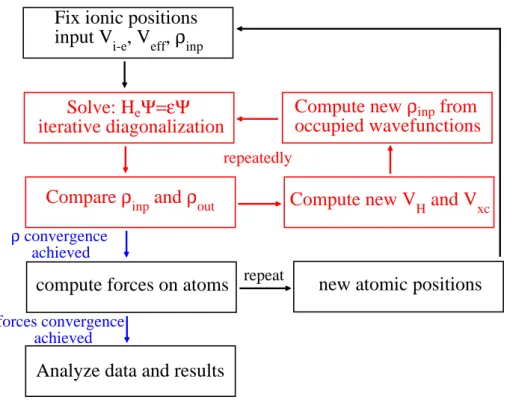
In Fig. 1.4 we show the flow-chart of the entire calculation, which summarizes the fundamental steps of the self-consistent approach in solving the total Hamiltonian and its electron and ionic parts. Starting from a given set of atomic positions in the unit cell and an initial guess of the electron density (generally obtained by a superpo-sition of atomic orbitals), the electronic Hamiltonian is solved self-consistently due to the dependence of the effective potential on the density. The convergence of the
Fix ionic positions
input V
i-e
, V
eff,
ρ
inpSolve: H
eΨ=εΨ
iterative diagonalization
Compare
ρ
inpand
ρ
outcompute forces on atoms
ρ convergence achieved
Analyze data and results
Compute new V
H
and V
xcCompute new
ρ
inpfrom
occupied wavefunctions
new atomic positions
forces convergence achieved
repeatedly
repeat
Figure 1.1: Self-consistent calculation flow chart. The electronic Hamiltonian is solved self-consistently and a new charge density is computed untill convergence (red scheme). The structural optimization is achieved through the calculation of the forces acting on atoms. They are moved untill the total force is less than the required threshold (black scheme).
electronic Hamiltonian is reached when the charge density difference between two consecutive steps is less than a given threshold. At this point, the ionic Hamiltonian is solved and the forces acting on atoms are computed. If these forces are higher than a given threshold, the ions are moved and a new set of coordinates determines the input ionic potential for a further electronic self-consistent calculation. When the forces acting on atoms are sufficiently low the computational process comes to end so that it is possible to extract the physical quantities of interest.
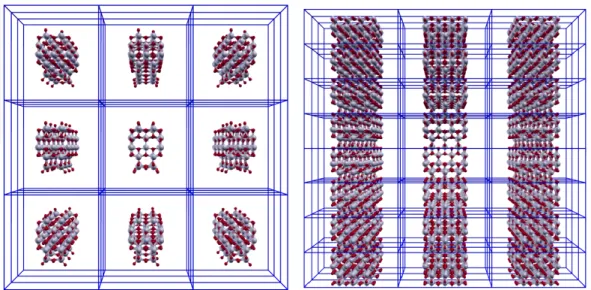
Figure 1.2: Pictures of the supercell approach. A vacuum region is introduced to avoid the interaction among the replica in neighbour cells. On the left a 0D TiO2 cluster is
surrounded by vaccum in each direction whereas on the right a 1D TiO2 nanowire is
surrounded by vaccum in the plane orthogonal to the growth direction.
1.5
Modeling low dimensional systems
The aim of this thesis is to present a detailed theoretical analysis of the proper-ties of TiO2 nanostructures, namely zero-dimensional clusters and one-dimensional nanowires (see Fig. 1.5). Thus their periodicity in real space is only present in the growth direction of the nanowires and absent in the clusters. In molecular chem-istry, and within an ab initio framework, such systems are predominantly calculated by means of codes which do not require the periodicity properties to simplify the computational demand. A given system is calculated as a whole and all the atoms (and their valence electrons) are explicitly treated. However, this approach brings some limitations to the size of the system that can be practically handled. Most of the calculations are actually performed on molecules of less than two-three hun-dreds atoms (this number rapidly decreasing with increasing number of electrons per atom). Furthermore, the accuracy of the calculation is often based on a skilful treatment of the basis set of the wave functions that represent the physical
quan-tities. Each atom has usually its specific set of localized wave functions, that can be modified according to the system and/or environment in which the atoms are placed. Hence the control over the convergence of the calculated quantities is not straightforward and sometimes becomes tricky.
On the contrary, our choice to use a plane wave based code allows a simple control of the convergence of the calculated physical quantities by increasing the number of the vectors in the basis set. When a three dimensional crystal is modeled, it is possible to uptake the Bloch theorem and thus to extract from a macroscopic ensamble of atoms its irreducible basis. It is made up of far less atoms (in a typical range of one-two tens) than the real crystal, but the latter is completely reproduced by the periodic replication in space of the irreducible basis. In the case of low dimensional systems it is possible to retain this approach if a vacuum region in the directions of non periodicity of the system is introduced into the unit cell (see Fig. 1.5). This vacuum gap must ensure that the atoms in the unit cell (or supercell ) do not interact with the neighbour replica, such that the system can actually be isolated.
Chapter 2
An overview of experimental
techniques and measurements
In this chapter, we summarize the basic aspects of the experimental methods used to synthesized TiO2 nanostructures through the description of those works we have relied on in this thesis. We also treat the experimental techniques used to measure both the structural and the electronic properties of these nanomaterials, paying particular attention to those works which have introduced still argued issues in the low dimensional physics of TiO2.
2.1
Synthesis of TiO
2nanostructures
The synthesis of TiO2nanostructures can be achieved following different techniques. New methods and variations on the existing procedures are constantly introduced, essentially to optimize the control over the parameters involved in the reactions and the quality of the final nanosample. On one hand, the main general efforts are to speed up the whole process, to obtain stable nanomaterials, and to keep the production costs low. On the other hand, it is necessary to control the fea-tures of the products in terms of their crystallinity, morphology, optical properties, photocatalytic activity, and more generally to optimize those properties that are mandatory for a good outcome of the final application the nanosample are made for. These aspects are often contrasting since a sufficient control of a given feature
of the nanostructure (e.g. blue shift of the band gap) can be linked with the effort in controlling a specific parameter of the synthesis process (e.g. size). In the follow-ing we summarize the most implemented and spread synthesis techniques of TiO2, advising the reader to refer to specialized publications for a deeper understanding of these techniques [11, 8, 35, 55, 56]. An accurate description of the large variety of works in this field goes beyond the purpose of the thesis.
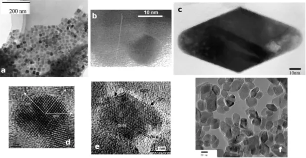
- Sol-gel Method is the most used technique to synthesize TiO2nanostructures. Gen-erally, a colloidal suspension (sol) is formed from the hydrolysis and polymerization of reacting precursors, which are typically inorganic metal salts or metal alkoxides. After a complete polimeryzation takes place the solvent is lost, leading to the tran-sition from the sol to the gel phase. In the case of TiO2 nanoparticles (NCs) it is possible to obtain a thin film on a substrate by coating. When the sol is cast into a mold a wet gel will form and then converted into a dense ceramic with further heat treatment. On the other hand, by removing the solvent in the wet gel, a pourous and low-density aerogel is obtained. In the case of TiO2 one-dimensional nanostructures (1D NWs), an anodic aluminum oxide template is immersed into the sol suspension, so that the sol will aggregate on the template surface and fill the channels to form high aspect ratio structures. With this technique, it is possible to exploit the varia-tions of the many parameters involved (reaction time, temperature, precursors, etc.) to vary the properties of the final nanosamples (shape, size, morphology, etc.). In Fig. 2.1 (a-c) we show the effect of varying the heating temperature and adsorbate species on the final morphology of the nanosamples.
- Solution Method is a nonhydrolytic sol-gel process that usually involves the reac-tion of titanium chloride with different oxygen donor molecules, as metal alkoxide and organic ether. As example, in the method used by Polleux et al. [57], TiCl4 was slowly added to a mixture of anhydrous benzyl alcohol and a ligand under vigorous stirring at room temperature and was kept at 80 ◦C for 24 hours in the reaction vessel. The resulting suspension was centrifugated and the precipitate was washed with chloroform. The collected material was left to dry in air at 600 ◦C and finally ground into a fine powder. The NCs were then assemblied to form TiO2 NWs in distilled water and by refluxing for 24 hours under stirring, see Fig. 2.2 (a-c). C. Liu and S. Yang [58] have very recently modified this method to synthesize the thinnest TiO2 NWs. They divided the process in a first step where the formation of the
Figure 2.1: a) TEM image of a cubic anatase TiO2 nanoparticles formed in a solution
of 0.10 mol dm−3 Ti(IV)-TEOA (1:2) compound at initial pH 10.5 and with 0.02 mol dm−3 sodium oleate [59]. b) TEM image of a spherical anatase nanoparticle obtained by heating at 375 ◦C for 3 hours [60]. c) HRTEM image of a bipyramidal anatase nanopar-ticle obtained heating at 240 ◦C for 64 hours [61]. d) HRTEM image of a spherical anatase nanoparticle synthesized with NaCl [62]. d) TEM image of a truncated tetragonal nanocrystal hydrothermally treated at 120 and 190◦C, then diluited in presence of tetram-ethylammonium hydroxide [63]. f) TEM image of nanoparticles obatined by hydrothermal treatment at 180◦C for 12 hours in double-distilled water [64].
precursors takes place and a second step in which the growth of the atomic wires is allowed by the presence of surfactants, see Fig. 2.2 (B-D).
- Hydrothermal method is usually performed in steel pressure vessels (autoclaves) with the optional use of Teflon liners under controlled temperature and pressure with the reaction in aqueous solutions. The temperature can be elevated above the boiling point of water, reaching the pressure of vapor saturation. The tem-perature and the amount of solution added to the autoclave largely determine the internal pressure produced. This method is widely used for the production of small particles in the ceramics industry. The Solvothermal method is almost identical to the hydrothermal one apart for the substitution of the water with another solvent.
Figure 2.2: On the left, a) HRTEM image of a trizma-functionalized trunacated bipyrami-dal domain; b) proposed morphology of the anatase nanocrystal; c) a chain of nanoparticles forming an anatase nanowire in the [001] direction [57], scale bar 2 nm. On the right, B) HRTEM micrograph of a single atomic wire with a diameter of around 4.3 ˚Aand lattice fringes spaced at about 3.5 ˚A, corresponding to the spacing between the (101) planes of anatase TiO2; C) HRTEM image of atomic wires with the corresponding FFT pattern in
the inset; D) Model structure of an anatase atomic wire growing along (001) direction [58].
However, the temperature can be elevated much higher than that in hydrothermal method, since a variety of organic solvents wih high boiling points can be chosen. The solvothermal method usually has better control of the size and shape distri-butions and crystallinity of the TiO2 nanoparticles than the hydrothermal ones, as shown in Fig. 2.1 (d-f).
Another well developed method deals with the direct oxidation of titanium metal using oxidants (peroxide) or under anodization (Direct oxidation method ). If ma-terials in a vaporate state are condensed to form a solid-phase material within a vacuum chamber through chemical reactions, the process is called chemical vapor deposition (CVD method ). In absence of chemical reactions the process is a physical vapor deposition (PVD method ). In CVD processes, thermal energy heats the gases in the coating chamber and drives the deposition reaction. Thick crystalline TiO2 films with grain sizes below 30 nm as well as TiO2 nanoparticles with sizes below 10
nm have been obtained with these techniques [8]. Other, more recent, techniques are the electrodeposition, the sonochemical method, and the microwave method.
2.2
Structural determinations
2.2.1
X-ray electron diffraction on powders
X-ray diffraction powder patterns come from the interference pattern of elastically dispersed X-ray beams by atomic cores and, in the case of materials with moderate to long-range order, contain information that arises from both the atomic structure and the particle characteristics (for example, size, strain). Alternatively, the radial distribution of the atomic pair distances in the material can be determined by the appropriate Fourier transform of the diffraction pattern independent of any require-ment of long-range coherence. This is an advantage in the study of nanoparticles or nanostructures in which there is reduced long-range order [11].
The lattice spacing (d) between crystal planes can be extracted using the Bragg law: 2d sin θ = nλ, where λ is the X-ray radiation wavelength, n is an integer number, θ is the reflection angle set equal to the incidence angle, d depends on the particular set of planes considered, as classified according to the Miller scheme [49]. The crystal lattice parameters can be measured by the above relation. In the ω− 2θ (or θ − 2θ) scan diffraction measurements, incidence and reflection angle ω and θ are changed simultaneously so that the condition ω = 2θ/2 is always satisfied (symmetrical configuration: here 2θ is the angle between the incident source ray and emerging ray, while ω is the angle between the sample surface and the incident ray). In Fig.2.3 the apparatus is schematically represented. When the reflection angle catches up the value for which the relation of constructive interference is satisfied, a strong signal is observed at the detector corresponding to a peak in the intensity vs. 2θ spectrum. When the measurement is carried out on a randomly oriented powder, the peak intensity depends on the intrinsic details of the crystal structure. Ideally, every possible crystalline orientation is represented equally in a powdered sample. The resulting orientational averaging causes the three dimensional reciprocal space that is studied in single crystal diffraction to be projected onto a single dimension. The three dimensional space can be described in spherical coordinates q, ϕ, χ. In
Figure 2.3: Schematic representation of an automatic diffractometer in the Bragg-Brentan geometry. S is the X-ray source, D the detector of diffracted ray, SP the sample holder.
powder diffraction, intensity is homogeneous over ϕ and χ and only q remains as an important measurable quantity. In practice, it is sometimes necessary to rotate the sample to eliminate the effects of texturing and achieve true randomness. When the scattered radiation is collected on a flat plate detector, the rotational averaging leads to smooth diffraction rings around the beam axis rather than the discrete Laue spots as observed for single crystal diffraction. The angle between the beam axis and the ring is the scattering angle 2θ. In accordance with Bragg’s law, each ring corresponds to a particular reciprocal lattice vector G in the sample crystal (G = 2πn/d). Powder diffraction data are usually presented as a diffractogram in which the diffracted intensity I is shown as function either of the scattering angle 2θ or as a function of the scattering vector q.
Li et al. [65] observed a contraction of the volume of anatase nanporaticle as function of decreasing size, by applying a standard least square method to calculate the cell parameters. On the other hand, Swamy et al. [13] found that the volume and the lattice parameter a of TiO2 nanosamples shorter than 10 nm underwent an increase with the size decrease, whereas the parameter c was found to contract. X-ray diffraction has been widely used to characterize the crystal phase of TiO2 nanosamples, from which it has been found that the anatase phase is thermody-namically favoured with respect to the rutile phase under 11 nm [8, 66]. From X-ray
diffraction it also possible to estimate the nanosample grain size according to the Scherrer equation
D = Kλ
βcos(θ) (2.1)
where K is a dimensionless constant and β is the full width at half-maximum of the diffraction peak. Nanocrystalline size is determined by measuring the broadening of a particular peak in the diffraction pattern associated with a particular planar reflec-tion from within the crystal unit cell. Nanoparticles are synthesized with diameters as small as 1 nm [67] and NWs with a diameter of 4.3 ˚A [58].
2.2.2
Extended X-ray absorption fine structure
This spectroscopy technique provide structural information about a sample by way of the analysis of its X-ray absorption spectrum. It allows determining the chemical environment of a single element in terms of the number and type of its neighbours, inter-atomic distances and structural disorders. This determination is confined to a distance given by the mean free path of the photoelectron in the condensed matter, in the Angstrom length scale. These characteristics make the extended X-ray absorp-tion fine structure spectroscopy (EXAFS) a powerful structural local probe, which does not require a long-range order. Furthermore, EXAFS does not require any particular experimental conditions, such as vacuum (at least in principle). There are several types of sample-holders that allow collecting experimental data under varying temperature and pressure, or while the sample is undergoing a chemical reaction (in-situ analysis) [69].
The X-ray absorption coefficient for an atom, indicated as µx, is directly propor-tional to the probability of absorption of one photon and is a monotone decreasing function of energy. It shows several discontinuities known as absorption edges, that occur when the energy of the incident photons equals the binding energy of one electron of the atom (classified as K, L, M... according to the principal quantum number n= 1, 2, 3...). The edge energy is characteristic of each atom. When the incident photon excite an electron with energy above the edge, it becomes an ex-tracted photoelectron that will be scattered by the atoms around the absorber. The
Figure 2.4: Schematic view of a X-ray beamline with synchrotron.
final state of the photoelectron can be described by the sum of the original and scat-tered waves. This leads to an interference phenomenon that modifies the interaction probability between core electrons and incident photons. The absorption coefficient will increase with constructive interference. Most importantly, the interference phe-nomenon, for a given energy of the photoelectron, depends on the distance between emitting and scattering atoms, and their atomic numbers. The EXAFS signal χ(k) is defined as a function of the wave vector k. It is mathematically defined as:
χ(k) = µx− µIx µIx
= µx µIx
− 1 (2.2)
where µx is the experimental absorption coefficient and µIx is the intrinsic atomic
absorption coefficient. Such a definition means that χ(k) contains only the oscilla-tory part of the absorption coefficient.
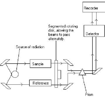
In a typical experimental set-up (Fig. 2.4) ionization cells monitor the intensity of incident (I0) and transmitted (I1) monochromatic photon beam through the sample, while scanning energy using a crystal monochromator (200 eV below to 1000 eV above the edge energy). The Lambert-Beer law relates intensities I0 and I to the absorption coefficient: ln(I0/I) = µx. Because of the angular rotation of the crystals inside the monochromator, the beam can shift up or down. Light must pass through the sample always at the same position, so either the sample follows the beam by placing it on a micrometric table, or it is necessary to change the monochromator mechanism to obtain a fixed beam.
For analyzing the EXAFS spectrum, we must separate the useful information (oscillation part) from the total raw spectrum. Then convert the oscillation part
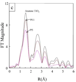
Figure 2.5: EXAFS spectra of bulk anatase TiO2 (black), a nanoparticle with a diameter
of 5 nm (P5, red curve), and a nanoparticle with a diameter of 11 nm (P11, violet curve) [18].
into k space by using the equation k = [0.263(EE0)]1/2, where E0 is the absorption edge. At last, the oscillation signal is filtered by Fast Fourier Transform and then fitted by the theoretical equation
χ(k) =∑ j Nj kr2 j | fj(k)| e−k 2σ2 je−2rj/λsin [ 2krj+ ϕ(k) + 0.2625rj∆E0 k ] (2.3)
where χ(k) is the filtered oscillation signal multiplied by a factor k3, j is the num-ber of the coordination shells, fj(k) is the amplitude value that can be obtained
from handbook, ϕ(k) is the phase displacement of scattering, ∆E0 is the difference between the theoretical value and the experimental value of the E0, N is coordina-tion number, r is coordinacoordina-tion distance, σ is Debye-Waller factor, and λ is electron mean-free path [70]. Fig. 2.5 shows an example of FT EXAFS spectra of TiO2 nanoparticles compared to the bulk anatase phase. The aim is to obtain the struc-tural parameters N , r, σ, and λ. Generally, the cubic spline interpolation method is used for the background removal and the least-squares method is used for the curve fitting. EXAFS is usually combined with X-ray absorption near edge spectroscopy
(XANES), the only difference being in the energy range of the final electronic state, which is lower than 50 eV in the latter case. XANES spectra also give purely electronic informations (e.g. chemical bonding). With these techniques experimen-talists found the distorsion of the octhaedral coordination of titanium atoms in TiO2 nanoparticles, resulting in variations of Ti-O atomic bond lengths, distances between atoms, and coordination numbers [14, 15, 16, 17, 18].
2.2.3
Transmission electron microscopy
If electrons are emitted in vacuum from a heated filament and accelerated through a potential difference of 50kV, their wavelength is about 1/20 ˚A so that they can penetrate distances of several microns into a solid. If the solid is crystalline, the electrons are diffracted by atomic planes inside the material, as in the case of x-rays. It is therefore possible to form a transmission electron diffraction pattern from electrons that have passed through a thin specimen. By focusing the transmitted electrons with electric or magnetic fields, the specimen can be imaged with a high spatial resolution [68].
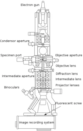
In a transmission electron microscope (TEM), electrons penetrate a thin spec-imen and are then imaged by appropriate lenses. These are stacked in a vertical column, as shown in Fig. 2.6. The source of electrons is a V-shaped filament made from tungsten wire, which emits electrons when heated in vacuum tube and tran-sistors control the lens currents and the voltage. The lenses of a TEM allow for beam convergence. Typically a TEM consists of condensor lenses that are responsi-ble for primary beam formation, of objective lenses that focus the beam down onto the sample itself, and projector lenses that are used to expand the beam onto the phosphor screen or other imaging device. The magnification of the TEM is due to the ratio of the distances between the specimen and the objective lens’ image plane. The vacuum system for evacuating a TEM to an operating pressure level consists of several stages. It is necessary to allow for the voltage difference between the cathode and the ground without generating an arc and to reduce the collision frequency of electrons with gas atoms to negligible levels. The most common mode of operation for a TEM is the bright field imaging mode. In this mode the contrast formation, when considered classically, is formed directly by occlusion and absorption of
elec-Figure 2.6: Schematic representation of the basic components of a TEM.
trons in the sample. Thicker regions of the sample, or regions with a higher atomic number will appear dark, while regions with no sample in the beam path will appear bright. The image is in effect assumed to be a simple two dimensional projection of the sample down the optic axis, and to a first approximation may be modelled via Beer’s law, more complex analyses require the modelling of the sample to include phase information.
Another imaging (usually bright field) mode of the TEM is the high-resolution transmission electron microscopy (HRTEM). It allows the imaging of the crystal-lographic structure of a sample at an atomic scale. Because of its high resolution, it is an invaluable tool to study nanoscale properties of crystalline material such as semiconductors and metals. HRTEM does not use amplitudes, i.e. absorption by the sample, for image formation. Instead, contrast arises from the interference in the image plane of the electron wave with itself. Due to our inability to record the
![Figure 2.2: On the left, a) HRTEM image of a trizma-functionalized trunacated bipyrami- bipyrami-dal domain; b) proposed morphology of the anatase nanocrystal; c) a chain of nanoparticles forming an anatase nanowire in the [001] direction [57], scale bar 2](https://thumb-eu.123doks.com/thumbv2/123dokorg/2844960.5513/32.892.161.769.203.484/functionalized-trunacated-bipyrami-morphology-nanocrystal-nanoparticles-nanowire-direction.webp)
![Figure 2.8: . FTIR spectra of anatase nanoparticles with a diameter of 11 nm (a, b, and c) and 16 nm (d, e, and f): hydrated, (a and d), evacuated at room temperature (b and d), and evacuated at 373 K (c and f) [28].](https://thumb-eu.123doks.com/thumbv2/123dokorg/2844960.5513/42.892.279.649.204.515/figure-spectra-nanoparticles-diameter-hydrated-evacuated-temperature-evacuated.webp)