Genetic Algorithm (GA) Based Techniques for 2D Microwave Inverse Scattering

UNIVERSITY

OF TRENTO

DIPARTIMENTO DI INGEGNERIA E SCIENZA DELL’INFORMAZIONE

38123 Povo – Trento (Italy), Via Sommarive 14 http://www.disi.unitn.it

GENETIC ALGORITHM (GA) BASED TECHNIQUES FOR 2D MICROWAVE INVERSE SCATTERING A. Massa

January 2002

Genetic Algorithm (GA) Based Techniques

for 2D Microwave Inverse Scattering

A. Massa

Department of Information and Communication Technology

University of Trento

Via Sommarive 14, I-38050 Trento, ITALY.

Phone +390461882057; Fax: +390461881696;

ABSTRACT

This paper deals with inverse scattering techniques based on genetic algorithms (GAs), and is devoted to microwave imaging and microwave nondestructive testing and evaluation (NDT/NDE). In the framework of near-field spatial-domain algorithms, a brief overview of current trends and future developments of the research work is given. Numerical results of selected simulations, modeling realistic geometries, are presented in order to assess the effectiveness of the proposed optimization methodology. Finally, a discussion fixes some guidelines and points out the open problems to be addressed in order to enlarge the application area of GA-based inverse scattering techniques.

I. INTRODUCTION

Microwave inverse scattering techniques are aimed at sensing a given scenario by means of interrogating electromagnetic waves in the range of microwaves. From a numerical point of view, the algorithmic aspects constitute the main obstacle to the development of efficient and practical reconstruction systems. At the present stage of their evolution, microwave imaging methodologies have limited applications to real-world problems (see [1, 2] and the references therein) and they are applied especially in research laboratories. However, non-invasive diagnostics by using low-power

electromagnetic fields could be very attractive in several area. Let us consider biomedical engineering [3, 4], non-invasive thermometry [5], geophysical analysis [6], archaeology [7] and industrial engineering [8] (e.g., nondestructive testing and evaluation [9,10]).

In order to allow a transfer from theory to practical imaging systems, the main theoretical difficulties are due to the ill-posedness and nonlinearity of the inverse scattering problem. As far as the ill-posedeness is concerned, the ‘golden rule’ for solving an inverse problem is the search for approximate solutions satisfying additional constraints coming from the physics of the problem. This information is usually called a priori information and the obtained solution is a regularized solution [11].

On the other hand, in order to take into account for multiple-scattering effects, a nonlinear model of the electromagnetic interactions between scatterers and probing fields must be considered. In the past, significant efforts were devoted to study numerical methods allowing the use of approximate relationships (e.g., Born-type approaches [12]). However, realistic scatterers to be inspected rarely are “weak” enough to allow the practical use of simplified techniques [13, 14]. Consequently, a lot of nonlinear inverse approaches have been proposed [15-18]. As far as the inversion procedures in the spatial domain are concerned, generally the solution of the problem is recast as the minimization of a suitable cost function. Very effective gradient-based iterative techniques have been successfully applied [19-21]. However, in this

case, a great care must be exercised due to the presence of local minima, which represent wrong solutions or artifacts, where the minimization algorithm can be trapped.

In the last few years, among optimization techniques, stochastic inversion procedures [22, 23] have gained great attention due to the rapid growth in computer technology. In particular, genetic strategies have shown their effectiveness in imaging two-dimensional dielectric [24, 25] or conducting scatterers [26, 27]. Generally speaking, GAs present typical characteristics very useful in dealing with microwave inverse scattering problems. Let us consider that:

• GAs are hill-climbing algorithms;

• GAs allow the straightforward introduction of a priori information (or constraints);

• GAs are able to deal with real and/or integer and/or binary unknowns at the same time;

• GAs are intrinsically parallel algorithms;

• GAs allow a hybridization with deterministic procedures.

However, in this framework, further researches are necessary in order to overcome some characteristic drawbacks of these approaches (e.g., large amount of computational burden, low convergence rate) allowing practical applications of microwave tomography to more complex industrial and medical applications.

In this paper, a review of a class of GA-based approaches for 2D microwave imaging is presented. The theoretical formulation is supported by some test cases involving canonical scatterers, showing the capabilities but also current limitations of the proposed techniques. A great emphasis is also given to the applications and different (customized) implementations of GAs are presented. Finally, a discussion closes this short review focusing on future trends of GA-based inverse scattering techniques.

II. MATHEMATICAL FORMULATION

Let us consider in a 2D geometry an inhomogeneous dissipative object embedded in a homogeneous lossless medium as shown in Fig. 1. The non-magnetic scatterer is characterized by a complex object function

( )

[

( )

]

( )

      ε π σ − − ε ε = τ 0 0 2 , 1 , , f y x j y x y x _R (1)

being ε the permittivity of the background, ₀ ε and σ R

the relative permittivity and the conductivity of the object, respectively. TM-polarized incident radiations,

V y

x

E_incν ( , );ν =1,..., _{, illuminate the investigation} domain, D. A multi-view/multi-illumination acquisition system is considered [28].

Figure 1. Two-dimensional problem geometry.

Under these conditions, the electromagnetic scattering process can be modeled by means of the following equations [29] D y x S y x dy dx y x y x G y x E y x k j y x E _{tot D} D scattν =

∫

τ( ,' ') ν ( ,' ') ( , / ,' ') ' ' ( , )∈ ,( , )∉ 4 ) , ( ₂ 2 0 _{(Data Equation) (2)} D y x dy dx y x y x G y x E y x k j y x E y x E _{tot D} D tot incν = ν −

∫

τ( ,' ') ν ( ,' ') ( , / ,' ') ' ( , )∈ 4 ) , ( ) , ( ₂ 2 0 _{(State Equation) (3)}

where S indicates the observation domain, E_scattν and ν

tot

E are the scattered and total fields related to the ν-th illumination condition, G_2D is the two-dimensional free-space Green’s function. The inverse scattering problem consists of determining the object function or its representation from the knowledge of the incident fields (E_incν ;ν=1,...,V _{) and of the scattered fields,} (E_scattν ;ν=1,...,V _{) collected in a set of measurement}

points (

(

x_m,y_m

)

;m=1,...,M) located in the observation domain. In order to numerically solve the system of equations (2)-(3), let us consider a representation of the unknown object function and of the electric field distribution. If the domain D is partitioned into N square sub-domains and E and _totν τ are taken to be piecewise constant in each subdivision of D, the discrete forms of the equations (2) and (3) result equal to

{ }

{ }

( , ) ( , ) ( , / , ) 4 ,..., 1 , ) , ( ) , ( 2 1 2 0 n n m m D N n n n tot n n m Data m m m Data m m scatt y x y x G y x E y x k j f M m S y x f y x E ν = ν ν

∑

τ = ℑ = ∈ ℑ = (4) being )G₂ν_D(x_m,y_m /x_n,y_n)=(jπk₀a_n /2)H₀(2)(k₀ρν_mn)J₁(k₀a_n and

{ }

{ }

( , ) ( , ) ( , / , ) 4 ) , ( ,..., 1 , ) , ( ) , ( 2 1 2 0 p p n n D N p p p tot p p n n tot n State n n n State n n inc y x y x G y x E y x k j y x E f N n D y x f y x E

∑

₌ ν ν ν τ − = ℑ = ∈ ℑ = (5) being

[

]

    ρ π − π = otherwise ) ( ) ( ) 2 / ( n = p if 2 ) ( ) 2 / ( ) , / , ( 0 1 0 ) 2 ( 0 0 0 ) 2 ( 1 0 2 p pn p p p p p n n D a k J k H a k j j a k H a k j y x y x G and where

{

x y E x y n N V

}

f = τ( _n, _n); _totν ( _n, _n); =1,..., ;ν=1,..., is the unknown array, J1 is the Bessel function of the

second kind, H₀( )2 _{and H} 1

2

( ) _{are the 0th and first order}

Hankel functions of the second kind, respectively; a_n = A_n/π , A_n being the area of the nth cell, ρpn is

the distance between the centers of the pth and nth cells and ρν

mn is the distance between the point (x ymν, mν) and

the center of the nth cell. Then, the approach involves the simultaneous solution of the system of equations (4) and (5). Let us consider the functional, Φ

( )

f =Φ_Data

( )

f +Φ_State

( )

f Φ (6) being

( )

{ }

∑∑

∑∑

= ν = ν = ν = ν _−ℑ = Φ _{V M} m m m scatt V M m m Data m m scatt Data y x E f y x E f 1 1 2 1 1 2 ) , ( ) , ( and

( )

{ }

∑∑

∑∑

= ν = ν = ν = ν _−ℑ = Φ _{V N} n n n inc V N n n State n n inc State y x E f y x E f 1 1 2 1 1 2 ) , ( ) , ( .

The basic idea of the approach is the iterative construction of a succession

{ }

f which converges to _k minimize the functional (6). To this end, a GA-based procedure is used.

III. GA-BASED INVERSION PROCEDURE

Genetic algorithms (GAs) are searching processes modeled on the concepts of natural selection and genetics. Their basic principles were first introduced by Holland in 1975 [30] and extended to functional optimization by De Jong [31]. GAs have been employed with success in a variety of problems in the field of applied and computational electromagnetics (see, for example, [32 - 34]). What makes GA’s immediately attractive is that they can be easily applied to problems involving non-differentiable functions and discrete as well as continuous spaces. These are qualities shared by other techniques, but GAs also exhibits an intrinsic parallelism. These features induced us to develop GA-based codes for microwave imaging purposes. The key points in designing a GA-based inversion procedure are:

• the design of evolutionary operators responsible for the generation of the trial solution succession,

{ }

f ; _k • the evolutionary procedure.

Different choices result in different inversion procedures able to efficiently deal with different microwave imaging problems.

1. BINARY GA-BASED INVERSION PROCEDURE (BGA)

Genetic Algorithms operate on a coding of the problem parameters. The GA, when applied to minimize the functional Φ

( )

f (equation (6)), requires the definition of a population of trial solutions

{

f p P

}

P₀ = ₀(p); =1,..., (7) being P the dimension of the trial solution population. Iteratively (being k the iteration number), the solutions are ranked according their fitness measures

( )

{

f p P

}

k K

F_k = Φ _k(p) ; =1,..., =0,..., (8) and, following the classical binary-coded version of the GA [35], coded in strings of N =N_par

(

log₂Q

)

bits, being Q the number of quantization levels used for each of the N_par unknowns

{

c p p P

}

k K

k

k = ( ); =1,..., =0,...,

Γ (9)

At this point, new populations of trial solutions are iteratively obtained by applying the genetic operators (selection, crossover and mutation) according to an evolutionary strategy [33]. For each iteration, firstly, a mating pool is chosen by means of a selection procedure

{ }

k S

k P

P( ) =ℵ (10) where ℵ indicates the selection operator. Then, a new population is generated applying, in a probabilistic way, the binary crossover and the binary mutation [24]

{ }

( ) ( )

{ }

( ) ) ( ) ( ) ( 1 S k M k S k C k M k C k k P M P P C P P P P = = ∪ = + (11)

The genetic operators are iteratively applied corresponding to their probabilities. Crossover is applied with a probability P , mutation is carried out _c with a probability P , the rest of the individuals are _m

reproduced. The iterative generation process stops if a termination criterion, usually based on a maximum number of generations, K (i.e., k≤K), or on a threshold on the fitness measure, δ (i.e., Φ

( )

(popt) ≤δ

k f being

( )

{

( )

( )

}

,..., 1 ) ( min _kp P p p k f f opt = Φ Φ = ), is verified.

The BGA works with a finite dimension parameter space. This characteristic makes the BGA ideal for optimizing a cost function arising from an inverse scattering problem where the unknowns (i.e., all the parameters or a part of the complete set of unknowns) can only assume a finite number of values. However, if a parameter is continuous, then it could be quantized [24]. The BGA works with the binary encodings, but generally in microwave imaging problems the cost function requires continuous parameters. Then, whenever the cost function is evaluated, the chromosome, c_k( p), must be firstly decoded. Moreover, if the number of binary-encoded parameters is large (as when an accurate discretization for the investigation domain is used) and if each parameter requires many bits to fully represent it, the size of the chromosome grows very quickly. On the other hand, BGA operators do not assure that the chromosomes of the next generation are admissible solutions. If acceptable solutions have to belong to some domains of the solution space (e.g., when constraints are imposed), monitoring this property under the action of the genetic operators can be laborious, and time-consuming (also in this case a decoding should be performed) and the convergence may therefore be slowed.

However, the binary encoding is not the only way to represent a parameter. Consequently, for microwave imaging applications, the BGA is only used when the unknowns are naturally quantized.

2. REAL GA-BASED INVERSION PROCEDURE (RGA)

When the parameters of the unknown array, f , are continuous variable, it is more logical to represent them by means of a real representation [37]. For RGA-based inversion procedures, a gene is the unknown itself and then ) ( ) ( p k p k f c = (12) Consequently, suitable genetic operators have to be defined in order to obtain admissible solutions and possibly enhance the convergence process. Of course, the design of variation operators has to obey the mathematical properties of the chosen representation, but there are still many degrees of freedom. However, also for inverse scattering problems, mutation must

remain a mean for a population to explore the parameter space randomizing the selected solutions and crossover must constitute a way to (randomly) mix the good characteristics of two chromosomes.

According to the evolutionary architecture proposed in [25], customized (to microwave imaging applications) genetic operators are then defined. As far as the RGA selection operation is concerned, a two step procedure is considered. Firstly, the new trial solutions,

) (

1

p k

f ₊ , not belonging to a physically reasonable space, are changed by recurring to the a-priori knowledge about the scenario under test (e.g., by imposing that

(

)

{

,

}

0

Reτk(p) xn yn ≥ and Im

{

τk(p)

(

xn,yn

)

}

≤0). Then a

standard tournament selection [38] works. This method gained increasing popularity because it is easy to implement, computationally efficient, and allows for fine-tuning the selective pressure [39] when inverse scattering problems are addressed.

Then the arithmetical crossover is performed. Arithmetical crossover is defined as a linear combination of two arrays. If (p1)

k

f and (p2)

k

f are two selected solutions to be crossed, the resulting offspring are

( )

( )

( ) ( ) ) ( 1 ) ( ) ( ) ( 1 2 1 2 2 1 1 1 1 p k p k p k p k p k p k f r f r f f r f r f + − = − + = + + ₍₁₃₎

being r a random variable uniformly distributed in the range [0, 1]. Finally, the RGA mutation is applied as follows η + = + ) ( ) ( 11 k p1 p k f f (14) being

( )

[

( )

]

{

( 1) min (p1) k i p k i i∈ f − f η ;max

[

( )

( 1)

]

( )

(p1)

}

k i p k i f f −

where f is the ith component of the unknown array _i f , and

(

min

{ }

f_i ,max

{ }

f_i

)

is its acceptance domain. 3. HYBRID-CODED GA-BASED INVERSION PROCEDURE

(HGA)

Sometimes in inverse scattering problems the a-priori knowledge about the scenario under test allows a parameterization of a subset of the unknown parameters by means of a small numbers of discrete parameters:

{

}

[ ]

L J L I l J j f_{l j} < < ∈ = ℜ = , 1 ,..., 1 ; l (15)

where I is the number of unknown parameters,

{

f i I

}

f = _i; =1,..., , and

{

l_j; j =1,...,J

}

is the set of discrete “equivalent” parameters. For those cases, a suitable encoding procedure must be defined in order to provide a one-to-one mapping between the parameter space and the chromosomes, but at the same time, exploiting the features of the unknown parameter set. To this end, in [40], a hybrid-encoding has been proposed. Integer-valued equivalent parameters,

{

l_j; j=1,...,J

}

, are binary coded and a floating-point representation is used for real unknowns,

(

)

{

f_t;t = L+1,...,I

}

. Then each unknown array, f , results in an hybrid-coded individual obtained concatenating the code of each parameter.

As far as the genetic operators are concerned, tournament selection and double point crossover [41] are used for selection and crossover, respectively. The mutation consists in perturbing, according to an assigned probability function P , only one element of _bm the chromosome. If the element is a bit, it is changed from 0 to 1 or vice-versa. Otherwise, the following mutation rule is considered

{ }

{ }

[

{ }

]

{ }

{ }

[

{ }

]

{ }

     − + ≥ − + = + otherwise f f r f r if f f r f f k t k t k t k t k t k t k t min 5 . 0 max ₁ 1 (16)

where r is a value generated by a pseudo-random ₁ number generator. In order to reduce the selection pressure and to keep the population diversity, when the difference between the fittest and the weakest individuals of the population is below a specified threshold, a refresh procedure is performed [42].

From the point of view of efficiency and effectiveness, the parameterization of a subset of the unknowns with a reduced number of representative parameters must be chosen in an effective way. The search space of the HGA-based inverse scattering procedure should be as small as possible without loosing the ability to express accurately, by means of the equivalent parameters, the original unknowns. If the parameterization function, ℜ, does not allow an accurate representation of the original unknown set, then it is impossible to retrieve it. With a correct parameterization, it is possible to add specific knowledge, about the addressed problem, to the GA-based inversion procedure, and effectively limit the search space (reducing the computational efforts) without limiting the accuracy of the reconstruction process. Furthermore, the parameterization method

should as effectively as possible prevent the creation of physically not admissible unknown arrays. A high number of invalid arrays among the reproduced individuals does not only mean wasted computation time, but it can severely disturb the mechanism of evolutionary search and cause a slow convergence rate. 4. HYBRIDIZED GA-BASED INVERSION PROCEDURES

Evolutionary algorithms are known as robust optimization techniques able to effectively explore very large nonlinear parameter spaces (the solution space of an inverse scattering problem is certainly very large – if an adequate resolution level is required – and highly nonlinear). As far as microwave imaging is concerned, GA-based procedures generally require a very high number of evaluations of the fitness function, thus offering poor performances in term of computational efficiency, especially when compared to deterministic optimization techniques. However, if the evaluation of the fitness function is computationally fast, evolutionary inverse scattering methods are very good candidates for a successful solution of the problem especially if the cost function is non-convex.

Different approaches to make GA-based procedures competitive with deterministic methods (while maintaining their favorable features) dealing with inverse scattering problems can be used. Certainly suitable encodings (Sect. 1, 2, 3) will reduce the solution space avoiding the search in some not-admissible regions. On the other hand, in order to save computational resources and to increase the rate of the convergence of the iterative approach, an effective strategy is the hybridization. Gradient-based minimization methods [43] usually converge very fast and yield very good reconstructions. However, in highly nonlinear problems, they can be trapped in local minima. In order to exploit complementary advantages of deterministic and stochastic approaches, GA-based procedures are coupled with a deterministic method. Two different methodologies can be adopted

• the RGA/CG-based approach;

• the approach based on the Memetic Algorithm (MA).

4.1. RGA/CG-BASED APPROACH (RGA/CG)

The simplest and more general way to realize a hybridized version of the inversion procedure is that of considering a two-stage optimization. Firstly, the reconstruction is performed with a GA (or a deterministic procedure), and subsequently switches to a deterministic procedure (or the GA). Different

strategies have been considered. In [44], a micro-GA has been coupled with a deterministic method proposing a communication criterion for stopping the stochastic algorithm and invoking the deterministic optimizer. Moreover, Ra et al. [45] proposed a hybrid optimization method combining the GA and the Levenberg-Marquardt algorithm (LMA) [46]. In this technique, the LMA is used to localize a minimum and then the minimization procedure switches to the GA in order to climb local minima. The procedure is repeated iteratively until the global minimum of the cost function is found.

On the contrary, following the idea preliminary presented in [25, 47], the proposed approach (RGA/CG) applies a GA and then a deterministic procedure, based on a conjugate-gradient algorithm, searches for the global optimum by virtue of its capacity of effectively refining and improving existing solutions [48]. In more details, the inversion procedure operates as a real-coded GA in order to locate the attraction basin of the global optimum. At each iteration, the “order of closeness“ to the global minimum [49] is evaluated and when a fixed threshold is achieved (k =k_CG), the following sequence of steps is performed:

the best trial solution obtained up to now ( ( opt) CG

p k

f ) is chosen as the initial estimate for a sequence of successive approximations generated according to a modified version of the standard Polak-Ribière conjugate gradient algorithm [43];

if the convergence threshold, δ, is not reached during the deterministic minimization, the RGA restarts by considering a population whose individuals are randomly generated around the current trial solution.

Selected numerical results, preliminary shown in [25], and some test cases, described in Sect. V, demonstrate the reliability and the effectiveness of this methodology.

4.2. MA-BASED APPROACH (MA)

However, in the author’s opinion a closer coupling between stochastic and deterministic optimizers (than the coupling offered from the two-stage procedure) could provide better reconstruction results. In this framework, the coupling could be obtained by introducing a genetic operator which performs a gradient-like based minimization (e.g., “hill-climbing” operator [48], G-Bit improvement [35], etc...). Another solution is the use of a class of GA-based hierarchical strategies. The general structure of a hierarchical strategy consists of two main levels

Basic level:

this level is responsible for the generation of new configurations.

Control level:

this level guides the basic level toward a global optimum solution.

In other words, the basic level performs a local optimization that is controlled by the control level in order to obtain an overall global behavior.

The MA is a hierarchical algorithm based on the concept of meme [50]. A meme is a unit of information that can be transmitted when people exchange ideas. Every idea is a trial solution, f (individual). Because of the ideas are processed before propagating them, each individual can be assumed as a local minima of the cost function. From an algorithmic point of view, the processing of an idea is simulated by means of a deterministic procedure and its propagation and/or evolution with a statistical GA-based technique. However, the main drawback of this methodology is that, if the number of unknowns is very large, the computational load is too heavy [51]. Nevertheless, some inverse scattering problems involve a limited number of unknowns. For these cases, the trade-off between computational burden and increase of the converge rate results again favorable and the MA-based approach outperforms other optimization techniques.

IV. NUMERICAL ASSESSMENT

The effectiveness and the capabilities, but also current limitations, of the class of the proposed inverse scattering techniques is assessed by means of many numerical simulations. Different fields of application will be considered in order to point out the large spectrum of the applications for the GA-based techniques, but also that an adequate customization is necessary in order to allow good performances and to achieve accurate reconstructions [52].

A. MICROWAVE IMAGING

Let us consider the geometry shown in Fig. 1. Microwave Imaging (MI) aims at retrieving the dielectric constant profile (i.e., the object function distribution) inside the investigation domain from a series of electric field measurements performed outside the region under test. For this application, RGA-based approaches demonstrated their effectiveness. Three examples have been selected to illustrate the present state of the art.

• Single Homogeneous Lossy Cylinder

As a first example, a lossy circular cylinder, (a =0.325λ₀ in radius, being λ the free-space ₀ wavelength) characterized by a constant object function

( )

x,y =τ_obj =1.2−1.85j

τ , is enclosed in a square

investigation domain L=1.125λ₀ in side. The investigation domain is partitioned into N = 81 sub-domains of equal size. V =4 unit TM plane waves successively illuminates the investigation domain. For each illumination (being θ_ν =(ν−1) ,π ν= ,...,

2 1 V the incident angle), the scattered electric field is collected at M = 40 measurement points lying on a circle of radius ρm =1.125λ₀ and uniformly distributed around the investigation domain. As far as the input scattered data are concerned, they are analytically available. The initial values of the object function for the inverse scattering procedure are always taken equal to the background value and the starting guess for the field distribution is chosen to be equal to the incident field. The assumed parameters for the GA-based procedures are: P = 81, Pc =0.6, 6Pm =0. , δ =10−4 and K =104.

The real part and the imaginary part of the true object function are presented in Fig. 2(a). Fig. 2(b) and 2(c), show the final convergent solution when the RGA and the RGA/CG are applied, respectively. It can be seen that the reconstruction obtained by the hybridized optimization algorithm is more accurate than the one provided by the RGA-based procedure, especially as far as the imaginary part is concerned. In order to quantitatively evaluate the reconstruction, the following error figures have been defined

(

)

(

)

(

)

∑

= ε _×         ε ε − ε = Ξ Nzone n act_{R n n} n n rec R n n act R zone y x y x y x 1 100 , , , (17)

(

)

(

)

(

)

∑

₌ σ _×         σ σ − σ = Ξ int 1 int 100 , , , N n act _{n n} n n rec n n act y x y x y x

where the N_zone can range over the investigation domain (N_zone = ), or over the cells belonging to the N scatterer (N_zone =N_int), or over the cells of the background (N_zone =N_out). Table I summarizes the obtained results showing also the error figures when a deterministic minimization (a standard CG algorithm) is performed.

1.2 Re

{

τ

( )

x,y

}

0.0 0.0 Im

{

τ

( )

x,y

}

-1.85 (a) 1.2 Re

{

τ

( )

x,y

}

0.0 0.0 Im

{

τ

( )

x,y

}

-1.85 (b) 1.2 Re

{

τ

( )

x,y

}

0.0 0.0 Im

{

τ

( )

x,y

}

-1.85 (c)

Figure 2. Reconstruction of a lossy circular cylinder. (a) Original cross-section. Reconstruction obtained with (b)

Procedure _Ξε

tot Ξεout Ξintε Ξintσ

CG 11.31 7.59 16.35 12.34

RGA 2.99 0.31 10.66 5.67

RGA/CG 1.22 0.17 4.2 1.78

Table I. Reconstruction of a lossy circular cylinder.

Error Figures. • Multiple Scatterers

In the second test case, three separated homogeneous cylindrical objects (Figure 3(a)) have been considered. The first square cylinder, centered at

0 325 . 0 1 1 =− c = λ c x

y , has an object function value

equal to τ₁ =2.0 and it is 0 26. λ -sided; the second ₀ square cylinder is centered at yc₂ = xc₂ =0.325λ₀ with

0 . 1 2 =

τ ; the rectangular cylinder (0 26. λ₀ ×0 39. λ₀)

is centered at 0.13 ₀ 3

3 =− c = λ

c y

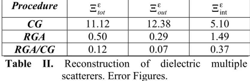
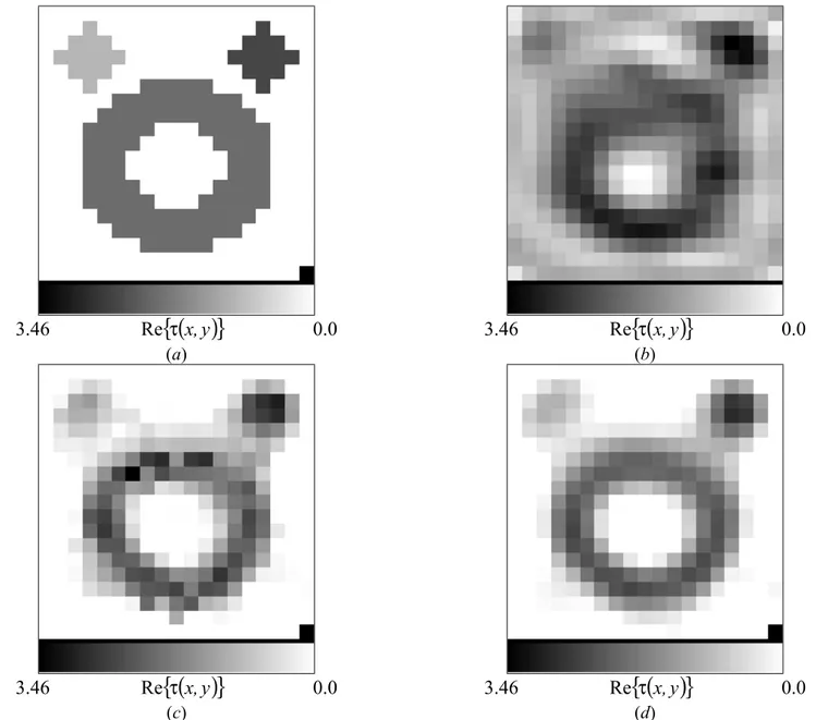
x with τ₃ =3.0. Concerning the input scattered data, they are synthetic data numerically computed by means of the Richmond’s procedure [53]. For the reconstruction process, we assumed that the variations in τ ranged between 0.0 and 4.0. Table II gives the error figures corresponding to the reconstructions shown in Fig. 3.

Procedure _Ξε

tot Ξεout Ξintε

CG 11.12 12.38 5.10

RGA 0.50 0.29 1.49

RGA/CG 0.12 0.07 0.37

Table II. Reconstruction of dielectric multiple

scatterers. Error Figures.

3.05 Re

{

τ

( )

x,y

}

0.0 3.05 Re

{

τ

( )

x,y

}

0.0 (a) (b)

3.05 Re

{

τ

( )

x,y

}

0.0 3.05 Re

{

τ

( )

x,y

}

0.0 (c) (d)

Figure 3. Reconstruction of dielectric multiple scatterers. (a) Original cross-section. Reconstruction obtained with (b)

Also the case of lossy scatterers has been taken into account. The values of the object function of the three cylinders was τ₁ =1.0−0.36j, τ₂ =0.6−1.25j, and

j 9 . 0 3 . 0 3 = −

τ . Figures 4, 5, and Tab. III confirms that GA-based inverse scattering procedures outperform standard deterministic CG-based methodologies.

Procedure _Ξε

tot Ξεout Ξεint Ξσint

CG 8.36 6.94 10.37 12.19

RGA 1.30 0.49 5.16 8.84

RGA/CG 0.19 0.05 0.87 4.50

Table III. Reconstruction of dissipative multiple

scatterers. Errors figures.

1.19 Re

{

τ

( )

x,y

}

0.0 1.19 Re

{

τ

( )

x,y

}

0.0

(a) (b)

1.19 Re

{

τ

( )

x,y

}

0.0 1.19 Re

{

τ

( )

x,y

}

0.0

(c) (d)

Figure 4. Reconstruction of the object function for dissipative multiple scatterers – Real part. (a) Original

cross-section. Reconstruction obtained with (b) CG-based approach, (c) RGA-based procedure and (d) RGA/CG-based procedure.

It should be pointed out that, in order to avoid the possibility that errors in the forward and inverse solutions may to cancel out, different discretization method have been considered to generate the synthetic scattered data and in the reconstruction algorithms. In

more detail, scattered data have been computed by considering a number of square domains equal to

20

20× corresponding to a discretization cell 0 5625 . 0 λ = ∆l -sided.

0.0 Im

{

τ

( )

x,y

}

-1.30 0.0 Im

{

τ

( )

x,y

}

-1.30

(a) (b)

0.0 Im

{

τ

( )

x,y

}

-1.30 0.0 Im

{

τ

( )

x,y

}

-1.30 (c) (d)

Figure 5. Reconstruction of the object function for dissipative multiple scatterers – Imaginary part. (a) Original

cross-section. Reconstruction obtained with (b) CG-based approach, (c) RGA-based procedure and (d) RGA/CG-based procedure.

Moreover, in order to assess the robustness of the proposed algorithms, the effect of the noise has been investigated. Numerically, the measurement noise has been simulated by adding to the scattered data a complex Gaussian random value with zero mean value and a standard deviation given by

( )

SN MV y x E M m V m m scatt 2 ) , ( 1 1

∑∑

= =ν ν = χ (18)

being

( )

S_N the signal-to-noise ratio. Table IV gives the errors figures computed at the end of the reconstruction process performed with the RGA/CG-based method.

(S/N) _Ξε

tot Ξεout Ξεint Ξσint

15 3.08 1.28 11.47 20.50

10 3.14 1.45 10.71 30.82

5 5.27 2.54 18.33 46.25

Table IV. Reconstruction of dissipative multiple

scatterers - Gaussian Noise. Errors figures. It can be observed that the retrieval results quite accurate for the permittivity profile. On the contrary, the quality of the reconstruction of the imaginary part of the object function strongly reduced when the signal-to-noise ratio decreases. As an example, Figure 6 shows the reconstructed image of the object function in correspondence with

( )

S_N =10dB.

1.46 Re

{

τ

( )

x,y

}

0.0 0.0 Im

{

τ

( )

x,y

}

-1.17

(a) (b)

Figure 6. Reconstruction of the object function for dissipative multiple scatterers – Noisy case (

( )

S_N =10 dB).

• Osterreich Configuration

Finally, a more complex environment, consisting of a modified version of the so-called “Osterreich” configuration, has been considered. Three different homogeneous scatterers, belonging to an investigation domain (L =1.0λ₀-sided), are imaged by considering

80 =

M input data collected in a circular measurement domain, ρ_m = L in radius. The permittivities of the scatterers are: εR₁ =2.0, 5εR2 =3. , and εR3 =3.0, respectively.

Figure 7 shows the object function distributions achieved at the end of the minimization process when different optimization strategies are considered. Table V gives some indications about the effectiveness of the hybrid optimization approach. In this case, the error figures do not result greater than 8%.

For completeness, in order to show the accuracy of the complete approach to predict the total electric field, Figure 8 gives color-level images of the amplitudes of the electric field inside the investigation domain and for the third view (ν = 3; θν =270 ). °

Procedure _Ξε

tot Ξεout Ξintε

CG 32.82 41.66 15.92

RGA 14.23 12.83 16.91

RGA/CG 6.82 7.32 5.18

Table V. Reconstruction of dielectric multiple

scatterers (Osterreich Configuration). Error Figures.

Reconstructed values (interpolated on a grid of 36 × 36 points) and actual values (computed by the Richmond’s procedure) show an excellent agreement.

3.46 Re

{

τ

( )

x,y

}

0.0 3.46 Re

{

τ

( )

x,y

}

0.0

(a) (b)

3.46 Re

{

τ

( )

x,y

}

0.0 3.46 Re

{

τ

( )

x,y

}

0.0

(c) (d)

Figure 7. Reconstruction of dielectric multiple scatterers (Osterreich configuration). (a) Original cross-section.

Reconstruction obtained with (b) CG-based approach, (c) RGA-based procedure and (d) RGA/CG-based procedure.

1.93 _Etotν

( )

_x,y ν=3 _{0.20 1.93}

( )

₃ totν x,y ν=

E 0.20

(a) (b)

Figure 8. Reconstruction of dielectric multiple scatterers (Osterreich configuration). Electric field amplitude (ν =3): (a) Actual distribution. Predicted amplitude achieved with the (b) RGA/CG-based procedure.

B. MICROWAVE NDT

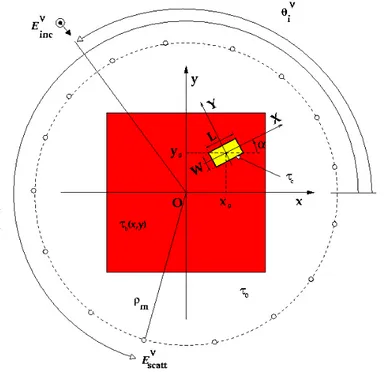
In order to illustrate the behavior of GA-based techniques for microwave NDT, let us consider a typical test case sketched in Fig. 9. An unknown defect (yellow area) is inside a known host medium (red area). Even if this scenario does not directly concerns material processing, it easy to imagine how it could be extended to such situations. The test sample (formally the investigation domain) is assumed to be cylindrical, as in the case of product conveyed in tubes, vessels or pipes. The sample is surrounded by a circular array of antennas forming a microwave scanner.

Figure 9. NDT problem geometry.

Starting from the knowledge of the scattered field due the presence of the defect, it would be possible to give a complete image of the scatterer. However, in NDE/NDT area a detailed imaging may often constitute a redundant information and faster computation or a simplified processing would be often preferred. The location and the shaping of the crack could be sufficient for an industrial monitoring of large-scale products. To this end, the inverse scattering procedure looks for the position, dimensions and orientation of the defect approximated by a void fixed shape. Then, by including the a-priori information about the scatterer under test, the crack-identification problem is that of finding the equivalent parameters of the crack

{

lj;j =1,...,5

}

≡

{

Lcrack,Wcrack,αcrack,x0,y0

}

(19)

(as shown in Fig. 9) and the electric field distribution for the flaw configuration. The discretization of the investigation domain in square sub-domains suggests the assumption that the equivalent parameters belong to finite set of values. Consequently, a hybrid encoding (i.e., a binary representation has been used for discrete parameters and a real-valued representation has been adopted for the electric field unknowns) is assumed and suitable genetic operators have been defined (Sec. 3).

0.1 A∆ 10 5 SNR 25 50 ξ 0 _c (a) 0.1 A∆ 10 5 SNR 25 100 ξ 0 _A (b)

Figure 10. Errors in the crack reconstruction for

different areas of the crack..

The effectiveness of the proposed approach (HGA), has been assessed by considering various operating conditions. In the first example, let us consider a square investigation domain

(

4λ₀/5

)

-sided. Firstly, the area,

A

∆ , of a void crack centered at point

(

₀/10

)

0 0 = y = λ

x is changed in the range between 0.1% and 10% of A (being A the area of the investigation domain) (Fig. 10). Then a crack having area equal to 0.04A has been moved along the diagonal of the investigation domain (Fig. 11). The measurement noise has been also taken into account and the signal-to-noise has been varied between 5 dB and 25 dB.

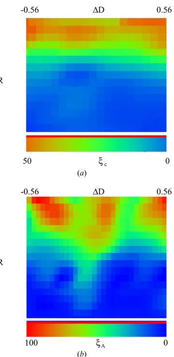
-0.56 D∆ 0.56 5 SNR 25 50 ξ 0 _c (a) -0.56 D∆ 0.56 5 SNR 25 100 ξ 0 _A (b)

Figure 11. Errors in the crack reconstruction for

different positions of the crack.

Figures 10(a) and 11(a) give an idea of the effectiveness of the HGA-based procedure in locating the crack (being ξ the percentage error in locating the _c crack). On the other hand, Figs. 10(b) and 11(b)

confirm also the capabilities of the method in shaping the crack (being ξ the percentage error in estimating _A the crack area).

C. MICROWAVE NDE

Let us consider the problem of determining the thickness of the layers of known (or partially known) materials deposed on a known specimen. This is an example of a typical problem arising in industrial NDE applications. In this case, the characteristic parameters of the scatterer (a multi-layer elliptic cylinder in Fig. 9) are almost completely known, however it is necessary to exactly estimate their value in order to certificate (or not) the quality of the product under evaluation.

Figure 12. NDE problem geometry.

By a mathematical point of view, the amount of a-priori information is very large and only a few parameters must be determined starting from the knowledge of the scattered electric field measured in the external observation domain.

As far as the elliptical geometry is concerned, the set of unknown equivalent parameters is

{

}

{

, 1,..., , 1,..., , , 0, 0

}

) 2 2 ( ,..., 1 ; y x d a a S S j S S j τ τ ≡ + × = l (20)

being S the number of layers,

(

x₀, y₀

)

the center of the cylinder, d the focal distance of the elliptic

cross-section and where a , _s τ , are the semi-major axis and _s value of the object function of the s-th elliptic layer, respectively. Moreover, the scattered electric field can be analytically computed as follows

(

) (

)

(

) (

)

∑

∑

∞ = + + + ∞ = + + + ν ϕ ς + + Ω Ψ = 0 1 1 ) 4 ( 1 0 1 1 ) 4 ( 1 v , u , v , u , ) v , u ( q m S q m S q S q q m S q m S q S q m m scatt h h o h h e E (21) where Ψ ,_q(4) (4) q

ς , and Ω , q ϕ are the radial and the q

angular Mathieu functions, respectively; S+1

q

e and S+1

q

o are scalar coefficients computed by means of a recursive procedure [54]; um and vm indicates the

coordinates of the m-th measurement point in an elliptic coordinate system..

Then the original inverse scattering problem (“to determine the object function in the overall investigation domain”) is recast to the minimization of the following cost function

( )

{ }

∑∑

∑∑

= ν = ν = ν = ν _−ℑ = Φ _{V M} m m m scatt V M m m Data m m scatt E f E f 1 1 2 1 1 2 ) v , u ( ) v , u ( (22) being f =ℜ

{

S,a₁,...,a_S,τ₁,...,τ_S,d,x₀,y₀

}

.

Because of the low-dimensionality of the solution space, it is expedient to apply the MA-based procedure. The proposed numerical implementation considers a conjugate-gradient method and a RGA as local and global minimizer, respectively. The iterative procedure performs the following tasks:

1. Initialize a starting population by creating a set of ideas,

{

f₀(p);p=1,...,P

}

;

2. Perform P local minimizations. Every current ideas is the starting point for a local minimization.

3. Perform selection, crossover and mutation according to the RGA-based procedure in order to produce the individuals of the next generation

{

f_k(₊p₁);p=1,...,P

}

;

4. Evaluate and assign the cost values to current ideas,

( )

{

f p p P

}

k(1) ; =1,...,

Φ ₊ ;

5. Iteratively repeat starting from task (2.) until

( )

≤δ

Φ (popt)

k

f .

In order to assess the effectiveness of the MA-based procedure, preliminary tests have been carried out. A three-layer elliptical cylinder (τ₁ =1.0 - internal layer,

0 . 4 2 =

τ and τ₃ =2.5 - external layer) illuminated by a line source placed at (−λ₀,0.0) has been considered. The scattered electric field has been collected at

21 =

M measurement points located along a probing line parallel to the y-axis, λ on the right of the ₀ scatterer. The following geometrical and dielectric characteristics have been considered: S =3,

0 1 =0.3λ

a , a₂ =0.4λ₀, a₃ =0.49λ₀, 0x₀ = y₀ =0. , and d =0.048λ₀. Table VI summarizes the results obtained from the reconstruction process. In order to reach the stopping threshold δ=10−5, only two iterations are necessary.

Step (k)

( )

) (popt k f Φ τ 1(k) τ (2k) (3 ) k τ 0 _1.39×10−1 _{18.474 1.0 5.0949} 1 _2.20×10−3 _{1.095 4.422 2.199} 2 _3.16×10−7 _{1.0 3.996 2.503}

Table VI. MA-based inverse scattering procedure.

Reconstruction of a dielectric multi-layer cylinder.

V. FINAL DISCUSSION AND CONCLUSIONS

In this paper, a number of methods based on a Genetic Algorithm has been reviewed. These approaches, developed in the spatial-domain, aim at solving the nonlinear inverse scattering problem of reconstructing the constitutive properties of bounded two-dimensional objects from values of the scattered fields on a surface entirely exterior to the scatterer under test, when the object is successively illuminated by known single-frequency incident fields originating

in different points of the exterior domain. All of the discussed methods involve minimizing the discrepancy between the actual measurements and a representation of the scattered field on the surface of measurements. In order to regularize the ill-posedness of the arising problem, a term proportional to the incident field in the investigation domain has been considered.

The difference in how the unknown object function is treated and how suitable GA-based procedures are implemented, is what distinguishes the various approaches. In developing these microwave imaging methodologies, it is clear that the following key issues must be addressed:

• A suitable representation and corresponding operators need to be developed when canonical representation is different from binary strings (BGA);

• Various constraints need to be taken into account by means of suitable method (ranging from penalty functions to repair the algorithms, constraint-preserving operators, etc...);

• A-priori knowledge about the scenario under test needs to be incorporated into the representation and the genetic operators in order to guide the search process and increase its convergence rate;

• A cost function needs to be developed which allows that its global minimum be the physical solution of the addressed inverse scattering problem;

• The parameters of the GA-based procedure need to be set (or tuned) and the feasibility of the approach needs to be assessed by comparing the solutions obtained by other deterministic and/or statistical microwave imaging procedures.

As far as the status-of-the-art of the application of GA-based microwave techniques to real-world problems is concerned, firstly it should be pointed out that evolutionary techniques in general and genetic algorithms in particular have had a relatively short history in the computational electromagnetics. However, it is a history that progressed rapidly. Actually, GA-based microwave imaging methods can not yet be considered as completely matured techniques (as well as other nonlinear methodologies in the framework of microwave imaging) if compared with well established imaging modalities such as ultrasound, infrared, X or gamma techniques. Several basic

questions have still to be answered before obtaining the degree of reliability required in industrial applications.

By a theoretical point of view, the questions of convergence and uniqueness of the solution needs some explanations. The theoretical foundations of GA-based methodologies are to some extent still weak. “We know that they work in microwave imaging, but we do not know precisely when the optimal solution will be achieved”: this is the typical idea of an user when a very complex problem is addressed and only a long heuristic training allow us to state some rules of thumb. Generally speaking this is not a constructive approach and it results as a limitation for real-world implementations. Moreover, the statistical nature of the GA operations is an effective characteristic, but on the contrary, a randomness in the definition of the evolutionary strategy represents an obstacle to industrial applications. Demystifying the optimal choice of GA parameters would be a great accomplishment. Adaptive parameters settings may be the solution [24], but much work is needed in this framework.

By a numerical point of view, severe limitations of the nonlinear inverse scattering methodologies are the computational load, the memory requirements and the rapidity of the reconstruction process. Certainly, the search space and the number of iterations of the minimization process evidently reduce in correspondence with an increase of the a-priori information. Indeed, if the initial guess profile is quite close to the actual contrast, the inverse scattering problem can be considered as quasi-linear allowing an increase of the convergence rate. However, a serious factor limiting the effectiveness of traditional deterministic approaches is their serial nature. On the other hand, GAs already possess an intrinsic parallel architecture and no extra efforts (as for deterministic procedures [55]) are required to construct a parallel computational framework. The GA-based methods can be fully exploited in their parallel structure to gain the required speed for industrial processing [56-58]. However, the use of parallel genetic techniques (PGT) is no different than other parallel systems, in which the computation performances are largely dependent upon the design of the system topology and communication links. Consequently, it is mandatory to take into account these factors in order to maximize the effectiveness of the GA-based microwave imaging approaches.

Nevertheless, even if further theoretical, numerical and experimental developments are still required for fully operational microwave imaging systems, existing equipments and known-how can be already suitably

used for preliminary practical applications (e.g., the “off-line” characterization of materials in laboratory or the “on-line” detection of defects in a specimen). Moreover, the flexibility of the proposed methodologies and the expected impact of such tomographic techniques largely justifies to devote a large research effort to develop GA-based tools dedicated to specific applications in the framework of microwave imaging and NDE/NDT applications.

REFERENCES

[1] Bolomey, J. Ch. 1996, Mat. Res. Soc. Symp. Proc., 430, 53-58.

[2] Bolomey, J. Ch., and Pichot, Ch. 1991, Int. Journ. Imaging Syst. Technol., 2, 144-156.

[3] Larsen, L. E., and Jacobi, J. H. 1986, Medical Applications of Microwave Imaging, IEEE Press., New York.

[4] Joisel, A., Mallorqui, J., Broqueras, A., Geffrin, J. M., Joachimowicz, N., Vallossera, M., Jofre, L., and Bolomey, J. Ch. 1999, Proc. 19th IEEE Instrum. Measurement Technol. Conf., Venice, Italy, 1591-1596.

[5] Bolomey, J. Ch., Le Bihan, D., and Miyakawa, M. 1995, in ThermoRadiotherapy and -Chemotherapy, Springer, Berlin, 361-379.

[6] Deming, R. W., and Devaney, A. J. 1997, Inverse Problems, 13, 29-45.

[7] Goodman, D. 1994, Geophysics, 59, 224-232. [8] Scott, D. M., and Williams, R. A. 1995, Frontiers

in Industrial Process Tomography, Engineering Foundation, New York.

[9] Zoughi, R., and Ganchev, S. 1995, Microwave NDE. State-of-the-Art Review, Austin, vol. 95-01. [10] Proc. Training Workshop on Advanced

Microwave NDT/NDE Techniques, Paris 7-9 Sept., France, 1999.

[11] Tikhonov, A. N., and Arsenin, V. Y. 1977, Solutions of Ill-posed Problems, Winston-Wiley, Washington.

[12] Maini, R., Iskander, M. F., and Durney, C. H. 1980, Proc. IEEE, 68, 1550-1552.

[13] Keller, J. B. 1969, J. Opt. Soc. Am. A, 59, 1003-1004.

[14] Slaney, M., Kak, A., and Larsen, L. E. 1984, IEEE Trans. Microwave Theory Tech., 32, 860-874.

[15] Habashy, T. M., Groom, R. W., and Speis, B. P. 1993, J. Geophysical Res., 98, 1795-1775.

[16] Chew, W. C., and Wang, Y. M. 1990, IEEE Trans. Medical Imaging, 9, 218-225.

[17] Kleinman, R. E., and van den Berg, P. M. 1990, Int. Journ. Imaging Syst. Technol., 2, 119-126. [18] Moghaddam, M., and Chew, W. C. 1992, IEEE

Trans. Geosci. Remote Sesnsing, 30, 147-156. [19] Kleinman, R. E., and van den Berg, P. M. 1992, J.

Comput. Appl. Math., 42, 17-35.

[20] Isernia, T., Pascazio, V., and Pierri, R. 1997, IEEE Trans. Geosci. Remote Sesnsing, 35, 910-923.

[21] Haruyuki, H., Wall, D. J. N., Takenaka, T., and Tanaka, M. 1995, IEEE Trans. Antennas Propagat.., 43, 784-792.

[22] Garnero, L., Franchois, A., Hugonin, J.-P., Pichot, Ch., and Joachimowicz, N. 1991, IEEE Trans. Microwave Theory Tech., 32, 860-874.

[23] Caorsi, S., Gragnani, G. L., Medicina, S., Pastorino, M., and Zunino, G. 1994, IEEE Trans. Antennas Propagat.., 42, 293-303.

[24] Pastorino, M., Massa, A., and Caorsi, S. 2000, IEEE Trans. Instrum. Meas., 49, 573-578.

[25] Caorsi, S., Massa, A., and Pastorino, M. 2000, IEEE Trans. Geosci. Remote Sensing, 38, 1697-1708.

[26] Chiu, C. C., and Liu, P.-T. 1996, IEE Proc., 143, 249-253.

[27] Qing, A., Lee, C. K., and Jen, L., 1999, J. Electromag. Waves Appl., 13, 1121-1143.

[28] Caorsi, S., Gragnani, G. L., and Pastorino, M. 1991, IEEE Trans. Microwave Theory Tech., 39, 545-551.

[29] Chew, W. C. 1994, Waves and Fields in Inhomogeneous Media, IEEE Press, Inc., New York.

[30] Holland, J. H. 1975, Adaptation in Natural and Artificial Systems, Univ. Michigan Press, Ann Arbor.

[31] De Jong, K. A. 1975, Ph. D. Dissertation, Univ. Michigan.

[32] Haupt, R. L. 1995, IEEE Trans. Antennas Propagat. Magazine, 37, 7-15.

[33] Johnson, J. M., and Ramat-Samii, Y. 1997, IEEE Trans. Antennas Propagat. Magazine, 39, 7-25. [34] Wiele, D. S., and Michielssen, E. 1997, IEEE

Trans. Antennas Propagat., 45, 343-353.

[35] Goldberg, D. E. 1989, Genetic Algorithms in Search, Optimization, and Machine Learning, Addison-Wesley, New York.

[36] Caorsi, S., Massa, A., and Pastorino, M. 1999, IEEE Trans. Antennas and Propagat., 47, 1421-1428.

[37] Janikow, C. J., and Michalewicz, Z. 1991, Proc. 4th Int. Conf. Genetic Algorithms, Los Altos, USA, 31-36.

[38] Goldberg, D. E., Korb, B., and Deb, K. 1989, Complex Syst., 3, 493-530.

[39] Bäck T. 1994, Proc. 1st IEEE Conf. On Evolutionary Computation, Piscataway, USA, 57-62.

[40] Caorsi, S., Massa, A., and Pastorino, M. 2000, Int. Journal of Applied Electromagnetics and Mechanics, 11, 233-244.

[41] Weile, D. S., and Michielssen, E. 1999, in Electromagnetic Optimization by Genetic Algorithms, John Wiley & Sons Inc., New York, 29-63.

[42] Caorsi, S., Massa, A., and Pastorino, M. 2002, IEEE Trans. Antennas Propagat., (in press).

[43] Polak, E. 1971, Computational Methods in Optimization, New York: Academic Press.

[44] Xiao, F., and Yabe H. 1998, IECE Trans. Electron., E81-C, 1784-1792.

[45] Yang, S.-Y., Choi, H.-K., and Ra J.-W. 1997, Microwave Optical. Technol. Lett., 16, 17-21. [46] Marquardt, D. W. 1963, J. SIAM, 11, 431-441. [47] Caorsi, S., Massa, A., and Pastorino, M. 2001,

Proc PIERS2001, Osaka, Japan, 223.

[48] Vanderplaats, G. N. 1984, Numerical Optimization Techniques for Engineering Design with Applications, Mc Graw-Hill, New York. [49] Caorsi, S., Massa, A., and Pastorino, M.,

submitted to IEEE Trans. Antennas Propagat. [50] Dawkins, R. 1976, The selfish gene, Oxford

University Press, Oxford.

[51] Merz, P., and Freisleben, B. 2000, IEEE Trans Evolutionary Comp., 4, 337-352.

[52] Wolpert, D. H., and Macready, W. G. 1999, IEEE Trans. Evolutionary Computation, 1, 291-299. [53] Richmond, J. H. 1965, IEEE Trans. Antennas

Propagat., 13, 334-341.

[54] Caorsi, S., Pastorino, M., and Raffetto, M. 1997, IEEE Trans. Antennas Propagat., 45, 575-560. [55] Mallorqui J. J. 1998, Proc. PIERS’98, Nantes,

France, 1017.

[56] Cantù-Paz, E. 1995, IlliGAL Rep., 95007, Illinois Genetic Algorithms Laboratory, Univ. of Illinois at Urbana-Champaign.

[57] Chipperfield, A. J., and Fleming, P. J. 1994, ACES Research Rep., 518, Univ. of Sheffield. [58] Davies, R., and Clarke, T. 1995, Control Eng.