Doctorate in
STRUCTURAL, GEOTECHNICAL ENGINEERING
AND SEISMIC RISK
XXXI CYCLE
Microstructure and mechanical
behaviour of cemented soils
lightened by foam
Domenico De Sarno
Supervisors
Prof. Gianfranco Urciuoli
Prof. Claudio Mancuso
PhD Coordinator
Prof. Luciano Rosati
help of Prof. Gianfranco Urciuoli, to whom I am very grateful. I would like to express my great appreciation to Prof. Claudio Mancuso, especially for his patience and comprehension.
I owe special thanks to Prof. Marco Valerio Nicotera, which has been extremely helpful in the interpretation of data, and Dr. Raffaele Papa, who was the first to believe in me, along with TERRE LEGGERE that provided all the materials.
I am very grateful to Prof. Giacomo Russo and Dr. Enza Vitale which have been fundamental in the whole part of the thesis devoted to microstructural and mineralogical analyses, in both tests and interpretation of data. Furthermore, the assistance provided by Enza in these years has been very valuable. I wish also to acknowledge the help provided by Dr. Dimitri Deneele in SEM observations.
Introduction ... 1
References... 4
Soil ... 7
Clay and clay minerals ... 7
Clay-water interaction ... 8
Diffuse layer models and clay particle associations ... 9
Rheological properties of clay suspensions ... 12
Bulk properties of soil slurry ... 17
Summary ... 18
References... 18
Cement and foam ... 20
Cement ... 20
Chemical composition and hydration reactions ... 21
Hardening and hardened paste structure ... 24
Effect of alkalis ... 25
Fillers and limestone Portland cement ... 26
Rheology of fresh paste ... 26
Bulk properties of cement paste ... 27
Foam ... 35
Surfactants ... 36
Surface tension and surfactant effect ... 37
Foam drainage and internal collapse ... 39
Bulk properties ... 41
Summary ... 41
References... 42
Governing parameters on behaviour of cemented soils ... 51
Lightweight cemented soil ... 53
Summary ... 55
References... 56
Materials and methods ... 62
LWCS bulk properties ... 62
Mix proportion design ... 70
Materials ... 74 Soil ... 74 Cement ... 76 Foam ... 77 Mix proportion ... 77 Specimen preparation ... 79 Summary ... 81 References... 81
Mineralogical and microstructural tests ... 83
XRD ... 83
TGA ... 85
Quantitative analyses of TGA ... 88
MIP ... 92
SEM ... 96
Discussion ... 100
Physical and mechanical properties of treated samples ... 103
Speswhite kaolin ... 103
Bulk properties ... 103
Caposele soil ... 149 Bulk Properties ... 149 Mechanical tests ... 152 Caposele-kaolin comparison ... 160 Failure surface ... 166 Discussion ... 170 References... 175
Summary and conclusions ... 177
Further developments ... 182 Appendix A ... 184 Clay minerals ... 184 Basic units ... 184 Mineral groups ... 186 References... 191 Appendix B... 192 Microstructural tests ... 192 X Ray Diffraction (XRD) ... 192
Thermogravimetric Analysis (TGA) ... 192
Scanning Electron Microscopy (SEM) ... 193
Mercury Intrusion Porosimetry (MIP) ... 193
Mechanical tests... 195
Oedometer test ... 195
Direct shear test ... 196
References... 198
Appendix C... 199
Lightweight cemented kaolin ... 217 Kcs40nf20 ... 218 Kcs40nf40 ... 221 Kcs20nf20 ... 233 Kcs20nf40 ... 235 Caposele soil ... 238
▪ 𝑉𝑠𝑙𝑢𝑟𝑟𝑦 volume of soil slurry; ▪ 𝛾𝑠𝑙𝑢𝑟𝑟𝑦 =𝑊𝑠𝑙𝑢𝑟𝑟𝑦
𝑉𝑠𝑙𝑢𝑟𝑟𝑦 bulk density of soil slurry;
▪ 𝑤𝑠 = 𝑊𝑤𝑠
𝑊𝑠𝑠
water content of soil slurry; o Solid
▪ 𝑊𝑠𝑠 weight of dry soil; ▪ 𝑉𝑠𝑠 absolute volume of soil; ▪ 𝜌𝑠 = 𝑊𝑠𝑠
𝑉𝑠𝑠 specific weight of soil;
o Liquid
▪ 𝑊𝑤𝑠 weight of water in soil slurry; ▪ 𝜌𝑤 specific weight of water; • Cement paste
▪ 𝑊𝑐 weight of cement paste; ▪ 𝑉𝑐 volume of cement paste; ▪ 𝑊𝑐,ℎ weight of hydrated cement; ▪ 𝑉𝑐,ℎ volume of hydrated cement;
▪ 𝑉𝑐,𝑝 total volume of pores in cement paste; ▪ 𝑉𝑐𝑎𝑝 𝑝𝑜𝑟𝑒𝑠 total volume of capillary pores; ▪ 𝛼 =𝑊𝑤𝑐,𝑛−𝑒𝑣
𝑊𝑐,𝑎,ℎ ;
▪ 𝛽 ≅ 0.746 parameter that takes account for shrinkage of non-evaporable water in cement paste;
▪ 𝑤𝑐 𝑐 ⁄ =𝑊𝑤𝑐
𝑊𝑐,𝑎 gravimetric water to cement ratio;
o Solid
▪ 𝑊𝑐,𝑎 weight of anhydrous (dry) cement (as a powder); ▪ 𝑊𝑐,𝑎,ℎ weight of the portion of initial anhydrous cement
(Wc,a) that is hydrated at a certain curing time, i.e. “anhydrous hydrated cement”;
▪ 𝑥 =𝑊𝑐,𝑎,ℎ
𝑊𝑐,𝑎 gravimetric portion of anhydrous cement
hydrated at a certain curing time;
time;
▪ 𝑉𝑐,𝑢𝑛ℎ𝑠 absolute volume of unhydrated cement; ▪ 𝑊𝑐𝑠 = 𝑊
𝑐,ℎ𝑠 + 𝑊𝑐,𝑢𝑛ℎ weight of solid cement paste; ▪ 𝑉𝑐𝑠 absolute volume of solid cement paste;
▪ 𝑊𝑐,ℎ𝑠 weight of solid products of hydration;
▪ 𝑉𝑐,ℎ𝑠 absolute volume of solid products of hydration; ▪ 𝑊𝑤𝑐,𝑐ℎ weight of chemically combined water;
▪ 𝑊𝑤𝑐,𝑛−𝑒𝑣 weight of non-evaporable water in cement paste; ▪ 𝑉𝑤𝑐,𝑛−𝑒𝑣= 𝑊𝑤𝑐,𝑛−𝑒𝑣
𝜌𝑤 volume of non-evaporable water;
o Liquid
▪ 𝑊𝑐𝑙 weight of liquid phase in cement paste; ▪ 𝑉𝑐𝑙 volume of liquid phase in cement paste; ▪ 𝑊𝑤𝑐 weight of water added to cement paste; ▪ 𝑉𝑤𝑐 volume of water added to cement paste; ▪ 𝑊𝑤 𝑐𝑎𝑝 𝑝𝑜𝑟𝑒𝑠 weight of water in capillary pores; ▪ 𝑊𝑤𝑐,𝑒𝑣 weight of evaporable water in cement paste; ▪ 𝑉𝑤 𝑐𝑎𝑝 𝑝𝑜𝑟𝑒𝑠 volume of capillary pores filled with water; ▪ 𝑊𝑔𝑒𝑙 𝑤𝑎𝑡𝑒𝑟 weight of gel water;
▪ 𝑉𝑔𝑒𝑙 𝑤𝑎𝑡𝑒𝑟 volume of gel water; o Gas
▪ 𝑉𝑐𝑔 volume of gas phase in cement paste; ▪ 𝑉𝑒 𝑐𝑎𝑝 𝑝𝑜𝑟𝑒𝑠 volume of empty capillary pores; • Foam
▪ 𝑉𝑓 volume of foam; ▪ 𝑊𝑓 total weight of foam; ▪ 𝛾𝑓 =𝑊𝑓
𝑉𝑓 bulk density of foam;
o Solid
▪ 𝑊𝑓𝑠 weight of solid phase in foam; o Liquid
▪ 𝑊𝑓𝑙 weight of liquid phase in foam;
▪ 𝜌𝑠𝑜𝑙𝑢𝑡𝑖𝑜𝑛 density of surfactant solution used to produce the foam;
• Lightweight cemented soil
▪ W weight of lightweight cemented soil; ▪ V volume of lightweight cemented soil;
▪ 𝑤 gravimetric water content of lightweight cemented soil; ▪ 𝑉𝑝 volume of pores of lightweight cemented soil;
▪ 𝑛 porosity of lightweight cemented soil; ▪ 𝑒 void ratio of lightweight cemented soil; ▪ 𝑐 𝑠= 𝑊𝑐,𝑎 𝑊𝑠𝑠 ; 𝑒𝑓 ′ = 𝑉𝑓 𝑉𝑠𝑜𝑖𝑙 𝑠𝑙𝑢𝑟𝑟𝑦+𝑉𝑔𝑟𝑜𝑢𝑡; 𝑛𝑓 = 𝑉𝑓 𝑉 ; ▪ 𝑒𝑏 =𝑉𝑐ℎ
𝑉𝑠 void ratio of bonds
▪ 𝛾𝑑𝑟𝑦(𝑛𝑓)
𝛾𝑑𝑟𝑦(𝑛𝑓=0)=
𝛾𝑑𝑟𝑦
𝛾𝑑𝑟𝑦,0 relative dry density
o Solid
▪ 𝑊𝑠weight of solid phase in lightweight cemented soil ▪ 𝑉𝑠 volume of solid phase in lightweight cemented soil ▪ 𝜌𝑠 =𝑊𝑠
𝑉𝑠 specific weight of solid phase of lightweight
cemented soil o Liquid
▪ 𝑊𝑙 weight of liquid phase in lightweight cemented soil; ▪ 𝑉𝑙 volume of liquid phase in lightweight cemented soil; ▪ 𝑊𝑤,𝑒𝑣 weight of evaporable water in lightweight cemented
soil;
▪ 𝑉𝑤,𝑒𝑣 volume of evaporable water in lightweight cemented soil;
o Gas
▪ 𝑉𝑔 volume of gas phase in lightweight cemented soil; ▪ 𝑉𝑎𝑖𝑟 𝑣𝑜𝑖𝑑𝑠 volume of air in lightweight cemented soil.
Clay Minerals Society”(Martin et al., 1991) ... 8 Figure 2-2. Diagrammatic sketch of electrical double layer. (a) Helmholtz
model; (b) diffuse layer model. ... 9 Figure 2-3. Representation of double layer repulsive forces (Frep) and attractive
van der Waals forces (Fatt) with distance. ... 11 Figure 2-4. Schematic representation of types of clay particle associations: (a)
Deflocculated and dispersed; (b) Deflocculated and aggregated; (c) EF flocculated and dispersed; (d) EE flocculated and dispersed (e) EF flocculated and aggregated (f) EE flocculated and aggregated (g) EE and EF flocculated and aggregated. (van Olphen, 1977). ... 12 Figure 2-5. Rheological behaviour in laminar flow. ... 13 Figure 2-6. Percentages of mass and volume in soil slurry for ws=140% and
ρs=2.59 [g/cm3] ... 18 Figure 3-1. Cement paste composition at different hydration states for Vc=40 ml
and Vwc=60 ml (Neville 2011). ... 30 Figure 3-2. Graphical representation of volumes in cement paste for 100 g of
anhydrous cement and wc/c=0.5 assuming Vwc,n-ev=Vwc ch; a) x=0, Vc,a=Vc,unh and Vwc=Vwc,ev; b) x=1, Vc,h=Vc volume balance given by (3-22); c) x=1, Vc,h=Vc volume balance given by equation (3-30). ... 33 Figure 3-3. Representation of weights and volumes in the cement paste for
Wc,a=100 g and wc/c=0.5... 34 Figure 3-4. Surfactant molecule sketch. ... 36 Figure 3-5. Diagrammatical sketch of (a) bubbles in foam, (b) plateau borders
and (c) foam lamella. ... 39 Figure 4-1. Schematic representation of compressibility behaviour of strongly
cemented soil, after Leroueil and Vaughan (1990), Cuccovillo and Coop (1999); PY: Primary Yield, PYCL: Post-Yield Compression Line (Rotta et al., 2003). ... 45 Figure 4-2. Schematic representation of compressibility behaviour of cemented
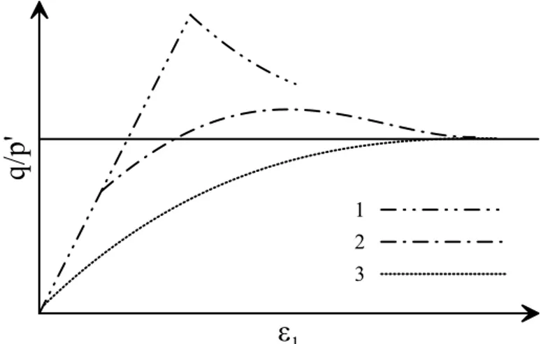
clay, after Sasanian and Newson (2014). ... 46 Figure 4-3. Idealized behaviour of cemented soil at different degree of
cementation, after Cuccovillo and Coop (1999), Lade and Trads (2014). 48 Figure 5-1 Graphical representation of mass and volume balances for Ws=100
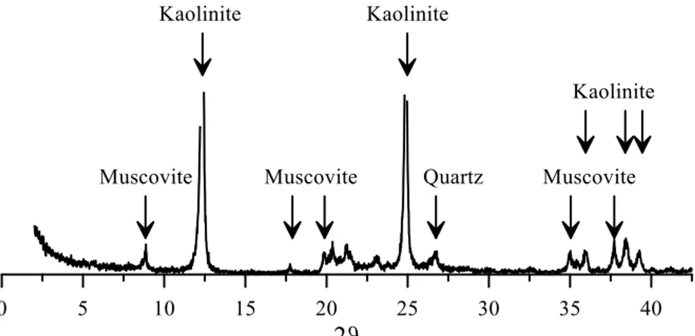
Figure 5-3. Grain size distribution of Speswhite kaolin and Caposele soil. ... 74 Figure 5-4. Results of X-Ray Diffraction analysis on Speswhite kaolin. ... 75 Figure 5-5. Results of X-Ray Diffraction analysis on Caposele soil; C: calcite,
M: muscovite, Q: quartz. ... 75 Figure 5-6. a) Fall cone test results. Solid lines refer to fit curves; vertical dotted
line refers to su at liquid limit, as suggested by Koumoto and Houlsby (2001); horizontal dashed lines refer to water content of soil slurry adopted for mixtures. b) Measured unit weight at varying water content. ... 76 Figure 5-7.Foam generator. ... 77 Figure 5-8. Graphical representation of theoretical composition of K cs40% nf
0-20-40%: (a) amounts of each component per cubic meter by weight; (b) percentages by volume. ... 79 Figure 5-9. Pictures of different stages of specimen preparation. The numbers
refer to the stage indicated in this section (5.3.5). ... 80 Figure 6-1. X Ray diffraction patterns of non-treated and cemented kaolin
(Kcs40) at different curing times. C, K, P, M refer to calcite, kaolinite, portlandite and muscovite, respectively. ... 84 Figure 6-2. X Ray diffraction patterns of non-treated and lightweight cemented
kaolin (Kcs40nf40) at different curing times. C, K, P, M refer to calcite, kaolinite, portlandite and muscovite, respectively. ... 84 Figure 6-3. Thermogravimetric analyses on anhydrous cement (CEM II/A LL
42.5R), Speswhite kaolin and cement grout (wc/c=0.5); P and K refer to Portlandite and Kaolinite, respectively. ... 86 Figure 6-4. Thermogravimetric analyses on Kcs40 at different curing times;
Speswhite kaolin (dotted line) and cement grout (dashed line) are also reported; P and K refer to Portlandite and Kaolinite, respectively. ... 87 Figure 6-5. Thermogravimetric analyses on Kcs40nf40 at different curing
times; Speswhite kaolin (dotted line) and cement grout (dashed line) are also reported; P and K refer to Portlandite and Kaolinite, respectively. .... 88 Figure 6-6. Evolution of portlandite with curing time by quantitative
interpretation of TGA analyses on Kcs40 and Kcs40nf40. ... 89 Figure 6-7. Evolution of the amount of non-evaporable water in time of treated
kaolin. ... 90 Figure 6-8. Evolution of αx with time and best fit of data. ... 91
days). ... 92 Figure 6-11. (a) Cumulative intruded volumes and (b) pore size distributions of
Kcs40 (cemented kaolin), Kcs40nf20 and Kcs40nf40 (lightweight
cemented kaolin) after 1 day of curing. ... 93 Figure 6-12. (a) Cumulative intruded volumes and (b) pore size distributions of
Kcs40 (cemented kaolin), Kcs40nf20 and Kcs40nf40 (lightweight
cemented kaolin) after 28 days of curing. ... 94 Figure 6-13. (a) Cumulative intruded volumes and (b) pore size distributions of
Kcs40 (cemented kaolin), Kcs40nf20 and Kcs40nf40 (lightweight
cemented kaolin) after 60 days of curing. ... 95 Figure 6-14. SEM observations on non-treated kaolin (a, b) and cement treated
sample (Kcs40 - c, d: 24h of curing; e, f: 60 days of curing) ... 96 Figure 6-15. SEM observations on Kcs40 (cement treated sample) at 60 days of curing. ... 97 Figure 6-16. SEM observations on Kcs40 (a, b, c), Kcs40nf20 (d, e, f) and
Kcs40nf40 (g, h, i) after 60 days of curing. ... 98 Figure 6-17. SEM observations on Kcs40 (a), Kcs40nf20 (b), Kcs40nf40 (c)
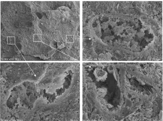
after 60 days of curing. ... 98 Figure 6-18. SEM observations on Kcs40nf40 (lightweight cemented samples)
at 60 days of curing time: details of air bubble footprint surface. ... 99 Figure 6-19. SEM observations on Kcs40nf40 (lightweight cemented samples)
at 60 days of curing: details of air bubbles filled by portlandite and cement hydrates. ... 99 Figure 6-20. SEM observations on Kcs40nf40 (lightweight cemented samples)
at 60 days of curing: details of cavities filled by portlandite and cement hydrates. ... 100 Figure 7-1. Comparison between estimated and measured value of (a) dry unit
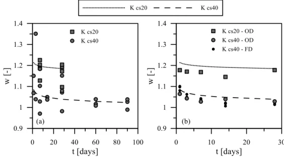
weight and (b) void ratio at different curing times. Dotted and dashed line refer to theoretical values. ... 105 Figure 7-2. Water content of cemented soil at different curing time. (a) Data
from samples after direct shear test; (b) data from oven dried and freeze-dried samples. ... 106 Figure 7-3. Comparison between estimated and measured (a) dry unit weight
and (b) void ratio of Kcs40nf 0-20-40 at varying curing time. Dashed lines refer to theoretical values. ... 108
Figure 7-5. Water content time evolution of Kcs40nf0-20-40. ... 109 Figure 7-6. Water content time evolution of Kcs20 nf0-20-40 oven dried
samples. ... 110 Figure 7-7. Direct shear tests on Kcs20 and Kcs40 at 7 days of curing. Dotted
and dashed lines refer to tests at 50 kPa and 100 kPa on non-treated kaolin, respectively. ... 111 Figure 7-8. Direct shear tests on Kcs20 and Kcs40 after 28 days of curing. ... 112 Figure 7-9. Direct shear tests on Kcs20 and Kcs40 at 𝜎𝑣’=100 kPa at 7 (dashed
lines) and 28 (solid lines) days of curing. ... 113 Figure 7-10. Direct shear tests on Kcs40 at 𝜎𝑣’=50 kPa at early stages of curing
(1, 3, 7, 14 days). ... 114 Figure 7-11. Direct shear tests on Kcs40 at 𝜎𝑣’=150 kPa at early stages of curing (1, 3, 7, 14 days). ... 115 Figure 7-12. Direct shear tests on Kcs40 at 𝜎𝑣’=150 kPa at different curing times
(7, 28, 60, 90 days). ... 116 Figure 7-13. Oedometric tests on Kcs20 and Kcs40 at 7 and 28 days of curing
(ε-log 𝜎𝑣’). ... 117 Figure 7-14. Oedometric tests on Kcs20 and Kcs40 at 7 and 28 days of curing
(e-log 𝜎𝑣’). ... 118 Figure 7-15. Comparison between oedometric tests on cemented and
non-treated kaolin (dotted line). ... 118 Figure 7-16. Direct shear tests on Kcs20nf40 after 28 days of curing at different vertical stress. ... 119 Figure 7-17. Direct shear tests on Kcs40nf40 after 28 days of curing at different vertical stress. ... 120 Figure 7-18. Direct shear tests on Kcs40, Kcs40nf20 and Kcs40nf40 at 𝜎𝑣’=100
kPa after 7 days of curing. ... 121 Figure 7-19. Direct shear tests on Kcs20, Kcs20nf20 and Kcs20nf40 at 𝜎𝑣’=100
kPa after 7 days of curing. ... 122 Figure 7-20. Direct shear tests on Kcs40, Kcs40nf20 and Kcs40nf40 at 𝜎𝑣’=100
kPa after 28 days of curing. ... 123 Figure 7-21. Direct shear tests on Kcs20, Kcs20nf20 and Kcs20nf40 at 𝜎𝑣’=100
kPa after 7 days of curing. ... 124 Figure 7-22. Direct shear tests at 𝜎𝑣’=50 kPa after 28 days of curing on Kcs20,
curing (1, 3, 7, 14 days). ... 127
Figure 7-25. Direct shear tests on Kcs40nf40 at 𝜎𝑣’=100 kPa at early stages of curing (1, 3, 7, 14 days). ... 128
Figure 7-26. Direct shear tests on Kcs40nf40 at 𝜎𝑣’=50 kPa at different curing times (7, 28, 60, 90 days). ... 129
Figure 7-27. Direct shear tests on Kcs40nf40 at 𝜎𝑣’ =100 kPa at different curing times (7, 28, 60, 90 days). ... 130
Figure 7-28. Comparison between oedometric tests on Kcs40 and Kcs40nf40 after 7 and 28 days of curing. ... 131
Figure 7-29. Comparison between oedometric tests on Kcs20, Kcs20nf40, Kcs40 and Kcs40nf40 after 28 days of curing. ... 132
Figure 7-30. Comparison between oedometric tests on cemented and non-treated kaolin (dotted line). ... 133
Figure 7-31. Effect of void ratio of bonds on peak strength of cemented kaolin, assuming φ=22° (non-treated kaolin). ... 135
Figure 7-32. Effect of void ratio of bonds on peak strength of cemented kaolin. ... 135
Figure 7-33. Direct shear test results on cemented kaolin in /σ-dh plane. ... 136
Figure 7-34. Effect of eb on lightweight cemented kaolin with nf=20%. ... 137
Figure 7-35. Effect of eb on lightweight cemented kaolin with nf=40%. ... 138
Figure 7-36. Effect of eb on cemented kaolin and lightweight cemented kaolin at varying nf. ... 138
Figure 7-37. Ratio of bond coefficient cb/cb0 against relative density. The dashed line is the fitting curve. ... 140
Figure 7-38. Representation of failure surfaces at constant 𝜎𝑣’ (50 – 100 – 150 kPa) given by (7-7) for φ = 27.6°, cb0 = 215 kPa, cf = 3.54. ... 141
Figure 7-39. Representation of failure surfaces at constant 𝛾𝑑𝑟𝑦 𝛾𝑑𝑟𝑦,0 (0.71 – 0.9 – 1) given by (7-7) for φ = 27.6°, cb0 = 215 kPa, cf = 3.54. ... 142
Figure 7-40. Comparison between measured and estimated lim in time (Kcs40). ... 142
Figure 7-41. Comparison between measured and estimated lim in time (Kcs20). ... 143
Figure 7-42. Comparison between measured and estimated lim in time (Kcs40nf20). ... 143
(Kcs20nf20). ... 144 Figure 7-45. Comparison between measured and estimated lim in time
(Kcs20nf40). ... 145 Figure 7-46. Comparison between measured and estimated lim in time, 𝜎𝑣’=50
kPa. ... 145 Figure 7-47. Comparison between measured and estimated lim in time, 𝜎𝑣’=100 kPa ... 146 Figure 7-48. Comparison between measured and estimated lim in time, 𝜎𝑣’=150 kPa ... 146 Figure 7-49. Theoretical evolution of UCS in time for CEM II/A 42.5R. Circles
refer to minimum strength at 2 and 28 days according to commercial datasheet. ... 148 Figure 7-50. Comparison between αx evolution in time derived by TGA
analyses and by evolution of UCS in time, assuming 62.5 MPa as
maximum strength. ... 149 Figure 7-51. Comparison between theoretical and measured dry bulk weight
and void ratio of cemented and lightweight cemented Caposele soil. ... 151 Figure 7-52. Comparison between theoretical and measured water content of
cemented and lightweight cemented Caposele soil. ... 151 Figure 7-53. Direct shear tests on Ccs40 at 𝜎𝑣’ equal to 50 and 150 kPa, at 7
(dashed lines) and 28 (solid lines) days of curing. ... 152 Figure 7-54. Direct shear tests on Ccs40nf20 at 𝜎𝑣’ equal to 50 and 150 kPa, at 7 (dashed lines) and 28 (solid lines) days of curing. ... 153 Figure 7-55. Direct shear tests on Ccs40nf40 at 𝜎𝑣’ equal to 50 and 150 kPa, at 7 (dashed lines) and 28 (solid lines) days of curing. ... 154 Figure 7-56. Direct shear tests on cemented and lightweight cemented Caposele soil at 7 days of curing and two vertical stresses (50 and 150 kPa). Dotted lines refer to non-treated Caposele soil. ... 155 Figure 7-57. Direct shear tests on cemented and lightweight cemented Caposele soil at 28 days of curing and two vertical stresses (50 and 150 kPa). Dotted lines refer to non-treated Caposele soil. ... 156 Figure 7-58. Unconfined compressive tests on cemented and lighweight
Figure 7-60. Comparison between oedometric tests on Ccs40 and Ccs40nf40 at 7 and 28 days of curing. ... 159 Figure 7-61. Direct shear tests. Comparison between cemented kaolin and
cemented Caposele soil, at different curing times and confining stresses. ... 160 Figure 7-62. Direct shear tests. Comparison between Kcs40nf20 and
Ccs40nf20, at different curing times and vertical stresses. ... 162 Figure 7-63. Direct shear tests. Comparison between cemented kaolin and
cemented Caposele soil, at different curing times and vertical stresses. . 163 Figure 7-64. Oedometric tests on cemented and lightweight cemented kaolin
and Caposele soil after 7 days of curing. ... 165 Figure 7-65. Oedometric tests on cemented and lightweight cemented kaolin
and Caposele soil after 28 days of curing. ... 166 Figure 7-66. Effect of foam on cb: comparison between kaolin (solid line) and
Caposele (dashed line). ... 167 Figure 7-67. Failure surface planes at constant 𝛾𝑑𝑟𝑦
𝛾𝑑𝑟𝑦,0, with cf=4, cb0=185 and
φ=29.4. Increasing 𝛾𝑑𝑟𝑦
𝛾𝑑𝑟𝑦,0, the amount of foam decreases. ... 168
Figure 7-68. Comparison between measured and estimated lim in time of cemented and lighweight cemented Caposele soil at two confining stresses. ... 168 Figure 7-69. Comparison between measured and estimated lim in time, 𝜎𝑣’=50
kPa. ... 169 Figure 7-70. Comparison between measured and estimated lim in time, 𝜎𝑣’=150 kPa. ... 169 Figure 8-1. αx time evolution of Speswhite kaolin mixtures. ... 178 Figure 8-2. Properties of mixtures (lines refer to theoretical values): a) bulk
weight (symbols refer to measured values); b) amount of cement per unit volume (symbols refer to corrected values 5.2.1.1). ... 179 Figure 8-3. Direct shear test results on different mixtures and curing times. .. 180 Figure 8-4. Direct shear test results: maximum shear strength at varying curing
time of Kcs40 and Kcs40nf40 in - 𝜎𝑣’ plane. ... 181 Figure 8-5. a) increase of cohesion with eb; b) relative reduction of cb with
Figure A-3. Diagrammatic sketch of tetrahedral sheet. (a) planar sketch; (b) bidimensional representation. ... 185 Figure A-4. Diagrammatic sketch of the octahedral sheet (Murray, 2006). .... 185 Figure A-5. Octahedron unit and bidimensional representation of Gibbsite and
Brucite. ... 186 Figure A-6. Representation of kaolinite structure. ... 187 Figure A-7. Pyrophyllite bidimensional representation and formula. ... 187 Figure A-8. Serpentine and talc bidimensional representations and formula. . 188 Figure B-1. Time-deformation curve in semi-log space (ASTM, 1990) ... 196 Figure B-2. Shear box apparatus (ASTM, 2003) ... 197
1
Introduction
The management of large amounts of excavated soil is a primary problem in civil engineering, often due to not suitable mechanical properties for its reuse as a construction material. Italian legislation defines the excavated soil and rocks (DPR 120/17) as the excavated soil deriving from activities aimed to a construction project such as excavations (construction excavations, foundations, trenches), bores, piles, soil improvement, infrastructural projects (tunnels, streets), removal and levelling of soil constructions. They can also contain concrete and cementitious mixtures, bentonite, PVC, fiberglass, and admixtures for mechanised excavations if pollutant concentration is below specific threshold. When the excavated soil is qualified as a waste, its disposal after a temporary storage must be considered in site management and high costs can derive. However, if the excavated soil can be reused as a material in the same construction project (or in a different one) for backfilling, trench reinstatement, soil embankments or substituting quarrying material in productive processes, it can be qualified as by-product with clear advantages in terms of environmental and economic costs.
A suitable solution for reuse of excavated soil is the addition of cement and foam to produce lightweight cemented soils (LWCS). Lightweight cemented soil is prepared by mixing soil with water, cement and an air foam. The aim of this technique is to obtain a material with high workability in the fresh state (so that it can be transferred by pumping from batch plant to the construction site and poured) improved mechanical properties of the hardened paste given by the binding agent (as cement) and a specific low density (varying from 6 to 15 kN/m3) thanks to the addition of a foam. The fresh paste is self-levelling and no compaction is required, thus reducing construction time. The method can be theoretically applied to any kind of soil except for very coarse particles which can segregate in the fresh paste. However, the necessity of such a method often arise for fine grained soil, especially clayey and silty soil, whose mechanical properties are generally not suitable for construction purposes or require high compaction efforts.
The treatment of soil by means of binding agents is nowadays very common in engineering practice. Well established soil improvement techniques as deep mixing, jet grouting and lime stabilization are based on mixing binding agents as cement and lime to improve soil mechanical performances. The former two are
2
grouped in the category of soil mixing, which is referred to as soil improvement and conditioning techniques in which soil is disrupted and mixed with binding agents via rotating utensils to obtain a “geomaterial” with specific geotechnical performances directly on site (Marzano, 2017). They are often used for columnar treatments, but also trench mixing techniques exist. A similar soil improvement technique is the permeation grouting, that is based on deep injection of cementitious mixtures at low pressure. It differs from soil mixing because no mixing of soil happens and a very little disturbance to soil fabric occurs (Flora and Lirer, 2011). In these cases, soil is not excavated. Conversely, cement and lime treatment (stabilization) techniques, as well as the lightweight cemented soil method, are used to improve soil mechanical properties to reuse it as a construction material. Cement and lime are the most commonly used binding agents in soil mixing, but others like fly ash and blast furnace slag, or the innovative geopolymers, can be used to substitute them, partially or wholly (Kaniraj and Havanagi, 1999; Wild et al., 1998; Zhang et al., 2013). In the LWCS method, the most common binding agent is cement, but also other binding agents have been efficiently used (S. Horpibulsuk et al., 2014).
A foam is a dispersion of bubbles in a liquid. In geotechnical engineering, foams are commonly used as a soil conditioner in Earth Pressure Balance (EPB) mechanized tunnelling technology. The addition of a foam has various purposes. It is used to make the soil almost impermeable and to reduce abrasive behaviour of some soils; it acts on consistency giving the soil a pseudoplastic state, to help muck circulation from excavation to its storage; in a fine grained soil, it is used to reduce clogging potential of clays and avoid overconsolidation under the action of the cutting edge of the screw (Quebaud et al., 1998). The effect of foam conditioning on soil properties related to EPB mechanised is widely studied (Borio et al., 2008; Milligan, 2000; Plötze et al., 2013; Sebastiani et al., 2017; Thewes et al., 2011; Zumsteg et al., 2012). In civil engineering, foam is also used to produce foam concrete (foamed concrete, foamcrete) that is a cellular concrete obtained by mixing a preformed foam with grout (like lightweight cemented soil method). It differs from gas-concrete, which is a cellular concrete usually obtained by adding aluminium powder to the paste. Foam concrete is a lightweight concrete whose density can go down to 300 kg/m3 along with strength which reduces as well; it is defined as a low density controlled low strength material and used for various applications such as backfills, void filling, insulation fills and pavement bases (Ramme, 2005). To avoid confusion, it is
3
worth noting that the term “foam” is also used to define dispersion of gas in solids, such as porous materials, cellular concrete and polymer foams, thus the lightweight cemented soil can be defined as a “foam” as well. However, in the following, the term foam will only refer to a gas dispersion in liquid.
The lightweight cemented soil method or lightweight treated soil method has been studied by various authors and efficiently applied on dredged soil in port construction in Japan (Tsuchida and Egashira, 2004), or suggested as a construction material for constructions on soft clays (Horpibulsuk et al., 2012b). The method requires that soil is diluted at a water content, ws, above the liquid limit, wl, to obtain a soil slurry, a suspension. The binding agent can be either added as a powder or mixed with water at a certain water to cement ratio by weight, wc/c. These two procedures are defined as dry and wet in soil mixing, respectively. By this way, a cemented soil can be obtained. The amount of binding agent is usually defined as the ratio by weight of anhydrous cement to dry soil, c/s, or to the volume of material produced. Foam is usually added as the last component. The amount of foam can be defined in different ways; in some cases, the volume of foam is related to the volume of soil slurry (Teerawattanasuk et al., 2015), in other cases to the total volume of soil slurry and foam (Horpibulsuk et al., 2012b). A diagram of the mixing method used in this study is represented in Figure 1-1.
Figure 1-1. Diagram of lightweight cement soil method.
In this experimental study, the influence of addition of cement and foam to soil on mineralogical and microstructural features is presented. Time dependent mineralogical and microstructural changes have been monitored at increasing curing time by means of X Ray Diffraction (XRD), Thermogravimetric Analysis
Water
Grout
Soil
Soil slurry
Lightweight Cemented Soil
Foam
Water
Cement
wc/cc/s ws
4
(TGA), Scanning Electron Microscopy (SEM) and Mercury Intrusion Porosimetry (MIP). Mechanical behaviour of treated soil has been investigated by means of oedometric and direct shear tests. Tests are briefly described in Appendix B.
In the following chapter a brief description of the main clay minerals, along with their structure and mineralogy, is presented. Then, clay-water interaction and rheological behaviour of clay suspensions, i.e., soil slurry, are shown. The 3rd chapter is about cement and foam. Cement classification, chemistry and rheology of the fresh cement paste are briefly summarized. A short description of foam properties and stability is given. In these chapters, the phases of each component (soil slurry, cement paste and foam) will be identified. The superscripts “s”, “l” and “g” will be used to specify respectively the solid, liquid and gas phases, the subscripts “s”, “c” and “f” will refer respectively to soil, cement and foam.
In the 4th chapter a literature review on the mechanical behaviour of cemented soils and lightweight cement soils is presented.
In the 5th chapter a description of materials and methods used in this study is given. The relations between the phases of the produced material in dependence of initial amounts of material are derived, starting from equations in Chapters 2 and 3 for each component.
The results of mineralogical and microstructural tests are presented in the 6th chapter. Direct shear test and oedometric test results are discussed in 7th chapter; in Appendix C, results of all the performed tests are shown.
References
Borio, L., Peila, D., Oggeri, C., Pelizza, S., 2008. Effects of foam on soil conditioned behaviour 1–8.
DPR 120/17: Regulation about the simplified discipline of the management of excavated soil and rocks, 13/06/2017 n° 120.
Flora, A., Lirer, S., 2011. Interventi di consolidamento dei terreni: tecnologie e scelte di progetto, in: AGI (Ed.), XXIV Convegno Nazionale Di Geotecnica Su “Innovazione Tecnologica Nell’Ingegneria Geotecnica”.
5
Horpibulsuk, S., Suddeepong, A., Chinkulkijniwat, A., Liu, M.D., 2012. Strength and compressibility of lightweight cemented clays. Appl. Clay Sci. 69, 11–21. https://doi.org/10.1016/j.clay.2012.08.006
Horpibulsuk, S., Wijitchot, A., Nerimitknornburee, A., Shen, S.L., Suksiripattanapong, C., 2014. Factors influencing unit weight and strength of lightweight cemented clay. Q. J. Eng. Geol. Hydrogeol. 47, 101–109. https://doi.org/10.1144/qjegh2012-069
Kaniraj, S.R., Havanagi, V.G., 1999. Compressive strength of cement stabilized fly ash-soil mixtures. Cem. Concr. Res. 29, 673–677. https://doi.org/10.1016/S0008-8846(99)00018-6
Marzano, I.P., 2017. Soil Mixing. Tecnologie esecutive, applicazioni, progetto e controlli, Argomenti di ingegneria geotecnica. Hevelius.
Milligan, G., 2000. Lubrication and soil conditioning in tunnelling, pipe jacking and microtunnelling. A state-of-the-art review. Rev. Lit. Arts Am. 44, 1– 46.
Plötze, M., Zumsteg, R., A.M. Puzrin, 2013. Effects of dispersing foams and polymers on the mechanical behaviour of clay pastes. Géotechnique 63, 920– 933. https://doi.org/10.1680/geot.12.P.044
Quebaud, S., Sibai, M., Henry, J.P., 1998. Use of chemical foam for improvements in drilling by earth-pressure balanced shields in granular soils. Tunn. Undergr. Sp. Technol. 13, 173–180. https://doi.org/10.1016/S0886-7798(98)00045-5
Ramme, B.W., 2005. ACI 229R-99 Controlled Low-Strength Materials 99, 1–15.
Sebastiani, D., Di Giulio, A., Miliziano, S., 2017. La gestione del condizionamento del terreno nello scavo meccanizzato di una galleria con TBM-EPB: risultati di una attività sperimentale, in: IARG - Incontro Annuale Ricercatori Geotecnica.
Teerawattanasuk, C., Voottipruex, P., Horpibulsuk, S., 2015. Mix design charts for lightweight cellular cemented Bangkok clay. Appl. Clay Sci. 104, 318– 323. https://doi.org/10.1016/j.clay.2014.12.012
6
Thewes, M., Budach, C., Bezuijen, A., 2011. Foam conditioning in EPB tunnelling. Geotech. Asp. Undergr. Constr. Soft Gr. - 7th Int. Symp. 127–135. https://doi.org/10.1201/b12748-19
Tsuchida, T., Egashira, K., 2004. The Lightweight Treated Soil Method: New Geomaterials for Soft Ground Engineering in Coastal Areas. CRC Press - Taylor & Francis Group, London.
Wild, S., Kinuthia, J.M., Jones, G.I., Higgins, D.D., 1998. Effects of partial substitution of lime with ground granulated blast furnace slag (GGBS) on the strength properties of lime-stabilised sulphate-bearing clay soils 51, 37–53.
Zhang, M., Guo, H., El-Korchi, T., Zhang, G., Tao, M., 2013. Experimental feasibility study of geopolymer as the next-generation soil stabilizer. Constr. Build. Mater. 47, 1468–1478. https://doi.org/10.1016/j.conbuildmat.2013.06.017 Zumsteg, R., Plötze, M., Puzrin, A. M., 2012. Effect of Soil Conditioners on the Pressure and Rate-Dependent Shear Strength of Different Clays. J. Geotech. Geoenvironmental Engineering 138, 1138–1146.
7
Soil
The lightweight cemented soil method can be applied to any kind of soil, except for coarse particles which can segregate from bulk. In this study attention was given to clayey soils, characterised by an amount of clay higher than 12% and non-negligible plasticity (ASTM, 2006). The behaviour of a clayey soil and its interaction with water are strictly related to mineral composition. Indeed. mineral composition and nature of constituent pore fluid can affect significantly some properties of a clayey soil, such as plasticity and residual strength (Di Maio and Fenelli, 1994, 1997). Due to this, clay minerals are briefly presented. Then, clay-water interaction and rheological behaviour of clay suspensions are shown, due to their importance in the treatment method which requires a dilution of clayey soil to obtain a slurry to be mixed with other components.
Clay and clay minerals
In geotechnics, the term clay refers to particles with diameter lower than 2 m (A.G.I., 1963), but in a more general definition, the term clay implies a “natural, earthy, fine-grained material which develops plasticity when mixed with a limited amount of water” (Grim, 1968). The plasticity is the property that a substance, continuously deformed under a finite force, has to maintain its shape after the force is removed or reduced (Andrade et al., 2011). Chemical analyses showed that clay minerals are composed essentially of silica, alumina, and water, with amounts of iron, alkalis and alkaline earths (Grim, 1968). The upper limit is dependent on the tendency of clay minerals to be concentrated in a size less than 2 m (Grim, 1968).
Clay minerals refer to a group of hydrous aluminosilicates that predominate the clay-sized (<2 m) fraction of soils (Barton and Karathanasis, 2002). The nomenclature and classification of these minerals have been discussed for many years (Grim, 1968). A classification is proposed by “The Clay Minerals Society” (Martin et al., 1991). A discussion about clay minerals classification goes beyond the purposes of the thesis; however, due to its importance, a brief description of clay minerals has been reported in Appendix A.
8
Figure 2-1. Nomenclature and classification of clay minerals, Copyright “The Clay Minerals Society”(Martin et al., 1991)
Clay-water interaction
The peculiar behaviour of clay when mixed with water depends on clay minerals structure and the high surface area of particles. As already shown in 2.1, the surface of clay minerals is composed of oxygen atoms or hydroxyl groups and excess electrons can arise from cations substitution in lattice (Grim, 1968). By this way, hydrogen covalent bonds can form between particle surface and water molecules, due to polarity of water. The totality of the negative electrical layer on the surface particles and the positive electrical layer in the adsorbed water is called electrical double layer.
9
Diffuse layer models and clay particle associations
In the simplest model, electrical double layer can be represented as composed of only two planes where all the electrical potential nullifies, proposed by Helmholtz as reported by Paunovic and Schlesinger (2006) (Figure 2-2a). However, due to counter-ions adsorption on particle surface, the counter-ions concentration is higher on the surface and lower in the bulk of solution. This causes a diffusive force of counter-ions towards the bulk solution, so that concentration of counter-ions is maximal near particle surface and decreases with distance. Moreover, due to electrostatic repelling force of surface, there is a deficiency of ions of the same sign of the surface charge around the layer. This is called diffuse layer model, called Gouy-Chapman model as reported by Paunovic and Schlesinger (2006) and it’s represented schematically in Figure 2-2b.
Figure 2-2. Diagrammatic sketch of electrical double layer. (a) Helmholtz model; (b) diffuse layer model.
The exact distribution of ions as a function of distance from the particle can be derived from electrostatic and diffusion theory. As concentration, the electric potential is maximum at the surface and decreases exponentially with distance. If the double layer is created by adsorption of potential-determining ions then the electrical potential, Φ, is expressed by Nernst equation (2-1) and, at a certain temperature T, it depends only on concentration of these ions in bulk solution, c, and the valence of ions, v:
𝛷0 = 𝑘𝐵𝑇 𝑣𝑒 ln ( 𝑐 𝑐0 ) ⇒ c = c0exp ( 𝑣𝑒𝛷0 𝑘𝐵𝑇 ) (2-1)
10
where kB is the Boltzmann constant and c0 is the concentration at zero point of charge when Φ=0 (van Olphen, 1977). As reported by van Olphen (1977), for small potentials at surface, the distribution of electric potential, Φ, with distance, x, from particle surface can be expressed as:
𝛷 = 𝛷0exp(−𝑘𝑥) (2-2)
where k is a constant inversely proportional to dielectric constant of the medium. These equations show that higher the counter-ion valences and concentration, lower is the electric potential and the diffuse layer is more compressed.
When two particles approach, due to their diffuse counter-ions, there is a repulsive force between them and work is required to move close two particles. However, also attractive forces exist, and flocculation demonstrate their existence. These forces are van der Waals attraction forces. According to van Olphen (1977), these forces are equal to the sum of all the attractive forces between every atom of one particle and every atom of the other particle and this summation lead to a less rapid decay with distance. Indeed, while van der Waals attractive force between two atoms is inversely proportional to the seventh power of the distance, it is inversely proportional to the third power of distance between two spherical particles (van Olphen, 1977). The attractive force is basically independent on solution, while repulsive forces depend on ion concentration and ion valence. As ion concentration decreases, as shown Figure 2-3 from a to c, suspension behaviour changes. In case a, which refers to a high ion concentration, if two particles come in contact, attractive forces are dominant, and flocculation occurs. In case c, at high distances, repulsive forces are dominant, and particles don’t flocculate; however, at much lower distances, attractive forces can be dominant, and coagulation takes place. Indeed, the sections that represent long-range repulsions are called “energy barriers” and particles that has passed the “barrier” are said to have “jumped over the barrier” (van Olphen, 1977). Case b represents an intermediate and unstable state.
11
Figure 2-3. Representation of double layer repulsive forces (Frep) and attractive van der Waals forces
(Fatt) with distance.
A more complex model for diffuse layer is the Stern model, that is a combination of Helmholtz and Gouy-Chapman models (Paunovic and Schlesinger, 2006). It assumes that some ions are restricted to a very small plane close to the particle surface (as the Helmholtz model) which cause a strong reduction of electric potential, while other ions are distributed in the solution, as Gouy-Chapman model.
The models shown in 2.2.1 can be applied to all suspensions. In the case of clay, the electric double layer structure is more complex due to clay mineral morphology. On the flat surface, a net negative charge due to ion substitution occurs. The compensating cations between unit-layers try to diffuse away in presence of water due to lower concentration, while they are attracted electrostatically to the charged lattice. These compensating cations act as counter-ions of the double layer, they are exchangeable for other cations and are confined in a narrow space between unit-layer surfaces. Due to the large adsorption force between lattice and counter-ions, conversely to other suspensions, a large portion of counter-ions is located on the surface while a smaller one is in the diffuse layer, with a better accordance to Stern model. On the edge surface, due to the abrupt disruption of tetrahedral and octahedral sheets, primary bonds are broken. It is likely that a positive double layer is created also on the edge surface.
Because of the plate-like morphology, when particles flocculate, three different particle associations may occur: Face to Face (FF), Edge to Face (EF) and Edge to Edge (EE).
12
Figure 2-4. Schematic representation of types of clay particle associations: (a) Deflocculated and dispersed; (b) Deflocculated and aggregated; (c) EF flocculated and dispersed; (d) EE flocculated and
dispersed (e) EF flocculated and aggregated (f) EE flocculated and aggregated (g) EE and EF flocculated and aggregated. (van Olphen, 1977).
Due to different double layers, their interaction changes in dependence of the kind of particle association. At the same time, due to different geometry, summation of van der Waals forces changes and, by consequence, the attractive force. As reported by van Olphen (1977), EE and EF associations lead to agglomerates that can be called “flocs”, while FF association can be called “aggregate”; dissociation of EE and EF particles is called “deflocculation”, while FF separation in thinner flakes can be called “dispersion”. This means that a suspension can be flocculated and dispersed or aggregated but deflocculated (Figure 2-4). Modes of clay particle association affect rheological behaviour of clay suspensions. In the following section, a brief explanation of rheological behaviour of suspensions and the influence of flocculation will be presented.
Rheological properties of clay suspensions
Given a unit cube of matter with a fixed lower surface named reference surface, if a shear stress is applied on the top surface, there is movement of the top layer in the same direction. The layer below moves in the same direction with a lower velocity and so on, which results in a velocity gradient in normal direction respect to shear stress direction. This gradient is called rate of shear, D, measured in sec-1. The rheological behaviour can be described by a relationship between shear stress and the rate of shear. When they are related by a linear relationship passing through origin, the fluid is called Newtonian (2-3). The constant of
13
proportionality is called coefficient of viscosity or briefly viscosity, , whose physical unit, in the International System, is Poiseuille (Pl), equal to 1∙Pa·sec. Water viscosity at 20 °C is 10-3 Pl, equal to 0.01 poise, another commonly used unit.
= 𝐷 (2-3)
Dilute suspensions behave as Newtonian fluids. The ratio between suspension viscosity, , and liquid medium viscosity, 0, is called relative
viscosity of suspension, r, and can be related to the amount of dispersed solids with a theoretical relation derived by Einstein, as reported by van Olphen (1977):
𝑟 = 1 + 𝑘𝑟𝐶𝑠 (2-4)
where Cs is the concentration of solids by volume and k
r is a constant equal
to 2.5 for spheres but it is much larger if particles are anisometric as plates or rods. The relation is valid only for suspension dispersed enough so that particles (large compared to molecules of medium) don’t influence one each other.
If solid concentration is high enough that interaction cannot be neglected, these formulas are no longer valid. Indeed, concentrated suspensions behave as non-newtonian fluids. Examples of non-newtonian behaviours are represented in Figure 2-5. In such systems, at each point, the apparent viscosity, /D, and
differential viscosity (or plastic viscosity), d/dD, can be defined.
Figure 2-5. Rheological behaviour in laminar flow.
When both apparent and differential viscosity increase with shear stress, the flow is defined as dilatant or shear thickening. In the opposite, when both apparent and differential viscosity decrease with shear stress, it is defined as
14
shear thinning. Thickening and thinning behaviours can be described by a power
law model (2-5), where K and n are two constants. If n < 1, it is shear thinning, with n > 1 it is shear thickening.
= 𝐾𝐷𝑛 (2-5)
If no flow occurs below a threshold shear stress 0, defined as yield stress, and differential viscosity decrease till a constant value where -D relation becomes linear, it is called Bingham pseudoplastic flow. Extrapolating the straight line to low shear rates, an ordinate B (called Bingham yield stress) is obtained. This linear behaviour is called ideal plastic flow or Bingham plastic
flow, described by equation (2-6).
= 𝐵+𝐷 (2-6)
= 0+ 𝐾𝐷𝑛 (2-7)
A shear thinning behaviour with an initial yield stress, 0, it’s also possible and there are different models which can describe this behaviour, as the Herschel-Bulkley which simply adds a yield stress to power model (2-7). It is worth noting that this representation of rheological behaviour is only valid in laminar flow, whereas turbulent flow occurs at high shear rates and behaviour is also determined by inertia forces.
These properties can be also dependent on shear history and shearing time. When apparent viscosity decreases with shearing time, it is called thixotropic; at the opposite, if apparent viscosity increases with shearing, it is called rheopectic. Some models can be used to predict the viscosity of a concentrated suspension, as the Einstein model for dilute suspensions (2-4). An example is the Krieger-Dougherty model (Krieger and Dougherty, 1959), in which Cs, max is the maximum solid concentration by volume, while [] is the intrinsic viscosity of suspension. As reported by Struble and Sun (1995), it takes account for the effect of individual particle on viscosity.
𝑟 = (1 + 𝐶𝑠 𝐶𝑠,𝑚𝑎𝑥
)
−[]𝐶𝑠,𝑚𝑎𝑥
(2-8)
2.2.2.1. Rheological behaviour of clay suspensions
The flow behaviour of dilute and concentrated clay suspensions is of the Newtonian and Bingham type, respectively. Indeed, flocculated particles are
15
linked together, thus a certain yield stress is developed. The behaviour can also be thixotropic.
Particle association presented in 2.2.1 affects the behaviour of a clay suspension. In a dilute clay suspension, viscosity increases if flocs are formed by EE and EF association, while it decreases when FF association occurs. In concentrated clay suspension, the continuous card-house structure given by EE and EF associations within the total volume leads to a Bingham behaviour. However, yield stress is reduced when FF association occurs simultaneously due to the lower links in the card-house structure.
In a pure water suspension, double layers are developed enough to prevent particle association by van der Waals attraction but, thanks to the opposite charge of edge and faces that exceeds the FF repulsion, EF association occurs with a T shape, leading to relatively high viscosity in dilute systems and high yield stress in concentrated systems. Salinity of water does affect the association and, by consequence, rheological properties. A low concentration of NaCl can lead to a compression of the double layer, diminishing both EF attraction and FF repulsion, leading to the breakage of the card-house structure and a reduction in yield stress and viscosity, respectively in concentrated and dilute clay suspensions. However, at higher salt concentration, due to further compression of double layer, van der Waals attraction forces between EE and EF association enhance and the card-house structure is more likely to occur, leading to an increase in viscosity and yield stress. At very high concentrations, yield stress can decrease again, maybe due to FF association by which card structure links are reduced. However, these effects depend on clay mineralogy and salt. By this way, flocculation or deflocculation can be fostered. There are cases in which a suspension must be fluid enough to be poured, but with a rather high concentration. In such a case, a lower viscosity and yield stress can be obtained by deflocculating the system by breaking EE and EF associations. This can be achieved by reversing positive-edge charge, determining an EE and EF repulsion (van Olphen, 1977).
In soil science, clay-water interaction is simply defined via Atterberg limits, which represent conventional boundary water content, w, between solid-plastic state, plastic limit wp, and plastic-liquid state, liquid limit wl, whose difference is defined as plasticity index Ip=wl-wp. These index properties are determined by means of standard procedures and are used for classification of fine grained soils (ASTM, 2006, 2005). The state is defined via the consistency index Ic=(wl-w)/Ip,
16
and liquidity index Il=(w-wp)/Ip. Even if the liquid limit is conventionally defined via Casagrande method, it has been shown that it can be related to a specific undrained shear strength, that is the water content at which undrained shear strength, su, of the remoulded soil is equal to 2 kPa (ASTM, 2005). Indeed, the liquid limit can be obtained also via the fall cone test, which allow to determine the undrained shear strength of a soil and it is standardized and preferred in many countries (Houlsby, 1982; Koumoto and Houlsby, 2001). Liquid limit can be assumed as the water content at which a 60°, 60 g cone penetrates 10 mm, corresponding to su=2 kPa. Indeed, undrained shear strength, su, can be determined as:
𝑠𝑢 =𝐾𝑊
ℎ2 (2-9)
Where h is the penetration depth, W is the weight of the cone and K is the fall cone factor, as defined by Hansbo (1957), which depends on cone geometry and roughness, as shown by Koumoto and Houlsby (2001), and it is equal to 0.30 for a 60° semi-rough cone. The relation between water content and undrained shear strength is nonlinear, as shown by Koumoto and Houlsby (2001) which propose the relation (2-10), linear in log(w)-log(su) plane, where pa is the atmospheric pressure.
𝑤 = 𝑎 (𝑠𝑢 𝑝𝑎)
−𝑏
(2-10)
They also suggest a fall cone undrained shear strength at the liquid limit equal to 1.4 kPa. The liquidity index and the undrained shear strength can be related to rheological properties of clay suspensions. Indeed, Locat and Demers (1988) show that a good relation exists between viscosity and liquidity index for different clays. They observe both Bingham and Bingham pseudoplastic behaviour; as expected, an increase in IL leads to a reduction of viscosity and yield stress. The authors identify a good relation between viscosity (in 10-3 Pl) and IL, proposing equation (2-11). About yield stress, not a unique relationship with IL seems to exist (converging at lower liquid index), but they only identify a range. However, for each soil, Locat and Demers (1988) find a linear relationship between log 0 – log su. They also propose a relationship between su and IL (2-12), whose expression is similar to (2-10).
= (9.27 𝐼𝐿
) 3.33
17 𝑠𝑢 = (19.8
𝐼𝐿 ) 2.44
(2-12)
Bulk properties of soil slurry
The soil, in its initial state, is a multiphase material composed of solid, liquid and gas phases. However, in the production process of the lightweight cemented soil, it is mixed with water at high water content, above liquid limit, to obtain a slurry. The initial structure of the soil is disrupted, particles are diluted, and a suspension is obtained; thus, slurry properties are, at least theoretically, independent of initial condition. If there is no air entrapped, then there is no gas phase. The subscript “s” refers to soil, while the superscript “s” refers to the solid phase of soil. With Wss and Vss respectively the weight and the volume of solid soil and Wws the weight of water in the slurry:
𝜌𝑠 = 𝑊𝑠 𝑠 𝑉𝑠𝑠 (2-13) 𝑤𝑠 = 𝑊𝑤𝑠 𝑊𝑠𝑠 (2-14)
where ws is the water content of soil slurry. Wws is the sum of initial water in soil and the water added to obtain a specific ws. Hence:
𝑊𝑠𝑙𝑢𝑟𝑟𝑦= (1 + 𝑤𝑠)𝑊𝑠𝑠 (2-15)
If the absence of voids and air entrapped is assumed, then: 𝑉𝑠𝑙𝑢𝑟𝑟𝑦 = 𝑉𝑠𝑠+ 𝑉 𝑤𝑠 = 𝑊𝑠𝑠 𝜌𝑠 + 𝑊𝑤𝑠 𝜌𝑤 = 𝑊𝑠𝑠 𝜌𝑠 + 𝑤𝑠𝑊𝑠𝑠 𝜌𝑤 = 𝑊𝑠𝑠(1 𝜌𝑠+ 𝑤𝑠 𝜌𝑤) (2-16) 𝛾𝑠𝑙𝑢𝑟𝑟𝑦 =𝑊𝑠𝑙𝑢𝑟𝑟𝑦 𝑉𝑠𝑙𝑢𝑟𝑟𝑦 = 1 + 𝑤𝑠 1 𝜌𝑠 + 𝑤𝑠 𝜌𝑤 (2-17)
where ρw is the density of water. Figure 2-6 shows the percentages of mass and volumes in a soil slurry for ws=140% and ρs=2.59 g/cm3.
18
Figure 2-6. Percentages of mass and volume in soil slurry for ws=140% and ρs=2.59 [g/cm3]
Summary
The behavior of clayey soil suspensions, the main constituent of the lightweight cemented soil, has been described in this section. The clay-water interaction strongly depends on clay mineralogy, which has been briefly described in Appendix A; the interaction between water and clay particles can be modelled by means of diffuse layer theory; at macroscale, the behavior can be modeled as a Bingham fluid. Depending on clay minerals, dilution (i.e. water content) and salts concentration different particle associations can occur, thus affecting the rheological behavior of clayey suspensions. Rheological properties (i.e. yield stress and viscosity) can be related to properties and state parameters commonly used in soil science, such as liquid limit and liquidity index.
References
A.G.I., 1963. Nomenclatura geotecnica e classifica delle terre.
Andrade, F.A., Al-Qureshi, H.A., Hotza, D., 2011. Measuring the plasticity of
clays: A review. Appl. Clay Sci. 51, 1–7.
https://doi.org/10.1016/j.clay.2010.10.028
ASTM, 2006. Standard Practice for Classification of Soils for Engineering Purposes (Unified Soil Classification System), ASTM Standard Guide. https://doi.org/10.1520/D2487-11.
ASTM, 2005. Standard Test Methods for Liquid Limit, Plastic Limit, and Plasticity Index of Soils, Report. https://doi.org/10.1520/D4318-10.
Barton, C.D., Karathanasis, A.D., 2002. Clay Minerals. Encycl. Soil Sci. 187– 192. https://doi.org/10.1081/E-ESS-120001688
Di Maio, C., Fenelli, G.B., 1997. Influenza delle interazioni chimico-fisiche sulla deformabilità di alcuni terreni argillosi. Riv. Ital. di Geotec. 695–707.
19
Di Maio, C., Fenelli, G.B., 1994. Residual strength of kaolin and bentonite: the influence of their constituent pore fluid. Géotechnique. https://doi.org/10.1680/geot.1994.44.2.217
Grim, R.E., 1968. Clay mineralogy, International series in the earth and planetary sciences. McGraw-Hill.
Hansbo, S., 1957. A new approach to the determination of the shear strength of clay by the fall-cone test, in: Swedish Geotechnical Institute Proceedings. pp. 1–59.
Houlsby, G.T., 1982. Theoretical analysis of the fall cone test. Géotechnique 32, 111–118. https://doi.org/10.1680/geot.1982.32.2.111
Koumoto, T., Houlsby, G.T., 2001. Theory and practice of the fall cone test. Géotechnique 51, 701–712. https://doi.org/10.1680/geot.2001.51.8.701 Krieger, I.M., Dougherty, T.J., 1959. A Mechanism for Non‐Newtonian Flow in
Suspensions of Rigid Spheres. Trans. Soc. Rheol.
https://doi.org/10.1122/1.548848
Locat, J., Demers, D., 1988. Viscosity, yield stress, remolded strength, and liquidity index relationships for sensitive clays. Can. Geotech. J. 25, 799– 806. https://doi.org/10.1139/t88-088
Martin, R.T., Bailey, S.W., Eberl, D.D., Fanning, D.S., Guggenheim, S., Kodama, H., Pevear, D.R., Środoń, J., Wicks, F.J., 1991. Report of the clay minerals society nomenclature committee: Revised classification of clay
materials, Clays and Clay Minerals.
https://doi.org/10.1346/CCMN.1991.0390315
Paunovic, M., Schlesinger, M., 2006. Fundamentals of Electrochemical Deposition, The ECS Series of Texts and Monographs. Wiley.
Struble, L., Sun, G.K., 1995. Viscosity of Portland cement paste as a function of
concentration. Adv. Cem. Based Mater. 2, 62–69.
https://doi.org/10.1016/1065-7355(95)90026-8
van Olphen, H., 1977. An introduction to clay colloid chemistry : for clay technologists, geologists, and soil scientists. New York.
20
Cement and foam
The lightweight cemented soil method requires the addition of two additives to soil slurry: cement and foam. The former is the binding agent, required to have the hardening of the paste, i.e. to gain strength. A summary of cement classification is reported below. Then, the main chemical compounds and reactions are presented. Finally, the structure and the different phases in the cement paste are widely discussed due to their considerable importance on lightweight cemented soil bulk properties. Foam is a dispersion of bubbles in a surfactant solution. It is added to lower the density, thanks to bubbles entrapped in the fresh paste during mixing, and to enhance workability. The main properties of foam and mechanisms of foam stability are discussed in this section.
Cement
Portland cement, named for resemblance of hardened paste to the Portland stone (a limestone near Dorset), was patented by Joseph Aspdin in 1824, but the prototype of modern cement was made in 1845 by Isaac Johnson (Neville, 2011). Nowadays, Portland cement represents the category defined as CEM I, in which its percentage has to be higher than 95%. Cements classified as CEM II are blend of Portland cement (which is the main constituent) with other materials, such as blast furnace slag, silica fume, pozzolana, fly ash, limestone. More generally they can be referred to as blended Portland cements. Blastfurnace cements, pozzolanic cements and composite cements are classified as CEM III, CEM IV and CEM V, respectively. They differ from blend cements in terms of percentages; for example, if blastfurnace slag percentage is below 35%, it is classified as CEM II Portland slag, if above, it is classified as CEM III Blastfurnace cement. The threshold in pozzolanic cements is 11%. Composite cements are composed of different materials. A letter, such as A, B or C, indicates that the amount of added material is within a specific range, while (for CEM II) a letter specifies the additional material, such as P for pozzolana and L or LL for limestone.
Cements are also classified in terms of minimum compressive strength in MPa at 28 days, which gives the name to the class: 32.5, 42.5, 52.5. These classes are subdivided in sub-classes depending on early stage strength whose minimum value depends on the resistance class. Cements with ordinary early stage strength are classified as Normal hardening and denoted by letter N, while cements with higher early age are classified as Rapid hardening cements and denoted by letter R.
21
Chemical composition and hydration reactions
The cement is manufactured primarily by burning up to 1450 °C a mix of calcareous material, such as limestone or chalk, and alumina and silica found as clay or shale and grinding the resulting clinker. These raw materials consist mainly of lime, silica, alumina and iron oxide.
The main components of cement are summarized in the following list. The name of compound, composition and abbreviation are reported. In cement chemistry, the following abbreviations are commonly used: CaO=C, SiO2=S, Al2O3=A, Fe2O3=F, H2O=H.
• Tricalcium silicate - 3CaO∙SiO2 ≡ C3S • Dicalcium silicate 2CaO∙SiO2 ≡ C2S • Tricalcium aluminate 3CaO∙Al2O3 ≡ C3A
• Tetracalcium auminoferrite 4CaO∙Al2O3∙Fe2O3 ≡ C4AF
It is worth noting that C2S can have at least three forms: α, β and γ. The former, α-C2S, inverts to β-C2S at 1450° C. This form, that is the one hydraulically active, is preserved in commercial cements, otherwise it further changes to γ-C2S at 670° C. The composition of cement can vary a lot, but the first two compounds usually constitute around 70% by weight. They can contain some oxides and impurities. In this case, the “impure” calcium silicates are defined as alite and belite, respectively.
Minor compounds, in terms of quantity, such as K2O, Na2O, MgO, TiO2, Mn2O3 constitute usually no more than a few per cent, but they can be of interest. The first two are known as “alkalis” and they have been found to react with some aggregates leading to disintegration of concrete and its rate of gain of strength (Neville, 2011). Gypsum (CaSO4∙2H2O) is also present; it is fundamental for workability of fresh past that is related to hydration of tricalcium aluminates.
The setting time is defined as the time at which the cement paste changes from a fluid to a rigid state, losing workability. This stiffening process is called “setting”. Initial and final setting time are two arbitrarily conditions that can be determined via the Vicat needle (ASTM, 2008). Hardening, which must be distinguished by setting, is the gain of strength of a set cement paste. Setting and hardening of cement paste depends on the hydration of these compounds, primarily C3S and C2S, and their products (products of hydration) that are insoluble in water.
22
The hydration process develops in time and its rate decreases continuously. The rate of hydration of the main compounds differ considerably. Calcium aluminates reactions are faster than calcium silicates. Calcium silicate hydration reactions can be assumed as the following, where C3S2H3 is a lower basicity calcium silicate and lime is separated as calcium hydroxide (portlandite), Ca(OH)2.
2𝐶3𝑆 + 6𝐻 → 𝐶3𝑆2𝐻3+ 3𝐶𝑎(𝑂𝐻)2 (3-1)
2𝐶2𝑆 + 4𝐻 → 𝐶3𝑆2𝐻3+ 𝐶𝑎(𝑂𝐻)2 (3-2)
The hydration of C3S is faster than C2S; rate of reaction can be defined as moderate and slow, respectively. The product C3S2H3 is usually referred as C-S-H gel. Indeed, there are uncertainties about the actual C:S ratio, and it is likely that products of C2S and C3S are slightly different, so the reactions above are derived by an assumption about CSH composition. The CSH is referred to as gel because it appears as amorphous, but electron microscopy shows a crystalline character. Its structure is very disordered and can appear often as composed of fibrous or flattened particles as some clay minerals, as suggested by Taylor (1950). In initial state of hydration, calcium hydroxide forms thin hexagonal plates of tens of micrometres. Later, the plates merge into a massive deposit constituting up to 25% of hardened paste.
Portlandite particles produced by hydration of calcium silicates, due to the limited solubility, are formed within interstitial space and, with a continuing supply of moisture, can react with silica thus producing additional hydration products of a fine pore structure (Newman and Choo, 2003). As reported by Bergado (1996), portlandite can react in soil-cement stabilization, and reactions, namely pozzolanic reactions, can be summarized by the following equations:
𝐶𝑎(𝑂𝐻)2+ 𝑆𝑖𝑂2 → 𝐶𝑆𝐻 (3-3)
𝐶𝑎(𝑂𝐻)2+ 𝐴𝑙2𝑂3 → 𝐶𝐴𝐻 (3-4)
These reactions depend on solubility of silicates and aluminates in soil; however, as stated by Bergado (1996), primary products of hydration (3-1, 3-2), are much stronger than the secondary ones, which produce a further additional cementing substance enhancing the bond strength between particles.
As already pointed out, the hydration of tricalcium aluminate is faster than calcium silicates. If sulphates are absent, its hydration leads to initial formation of calcium aluminium hydrate, C4AH19, and subsequently C3AH6 (Black et al., 2006); the chemical reaction can be assumed as the following: