1933: Radio Signals From Sagittarius [Historical Corner]

2019

Publication Year

2020-12-14T15:37:56Z

Acceptance in OA@INAF

1933: Radio Signals From Sagittarius [Historical Corner]

Title

NESTI, Renzo

Authors

10.1109/MAP.2019.2920050

DOI

http://hdl.handle.net/20.500.12386/28835

Handle

IEEE ANTENNAS & PROPAGATION MAGAZINE

Journal

61

Number

HISTORICAL CORNER

1933: Radio Signals From Sagittarius

Renzo Nesti

T

he title of the front-page left head-line of the 5 May 1933 issue of the

New York Times (Figure 1) was

“New Radio Waves Traced to Centre of the Milky Way.” This was the world-wide announcement of Karl Guthe Jan-sky’s (Figure 2) discovery of radio waves apparently coming from the center of our galaxy.

Today, this announcement is cele-brated as the birth of a new science, radio astronomy. But at that time, it was not known that celestial objects could emit radio waves detectable from Earth, and this particular kind of radio detection was not the purpose of Jansky’s experiments. The first detection of radio waves coming from outside Earth was an event made possible by a mixture of luck, technologi-cal capabilities, and human abilities along with Jansky’s skill, persistence, and deep curiosity in investigating the new.

Besides the papers by Jansky, the key references for this landmark in astronomi-cal research are the book by W.T. Sullivan (1984) [1] and the paper by W.A. Imbriale (1998) [2]. The originality of the pres-ent work is mainly to revisit the electro-magnetic modeling of the Jansky antenna with modern software tools, present some crucial pictorial views of the sky seen by Jansky during his experiments, and focus

Digital Object Identifier 10.1109/MAP.2019.2920050 Date of publication: 6 August 2019

EDITOR’S NOTE

This issue’s “Historical Corner” column is about the first-ever detection of radio signals of extraterrestrial origin. It is focused on the Holmdel measurement campaign in the 1930s, highlighting the technological background leading to Jansky’s detection of that hiss-type signal being celebrated as the birth of radio astronomy. What would have been a detailed report of a successful experiment on the characterization of thunderstorm static, it has the flavor of a happy-ending

fairy-tale chapter of a book on a branch of science whose writing is in continuous progress. We are almost necessarily led to increase our interest in every minute detail of that historical campaign if we let our mind recall all the discoveries made by radio astronomers, improving our knowledge of the universe. The very last of these has

Giuseppe Pelosi

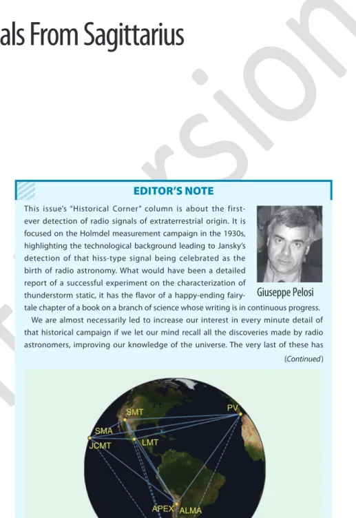
FIGURE S1.

A map of radio telescopes across the world contributing to the Event

Horizon Telescope. [Source: Event Horizon Telescope Collaboration/Astrophysical

Journal Letters, 875(2019) L1/CC BY 3.0.] SMT PV LMT JCMT SMA APEX ALMA SPT (Continued )

110 A U G U S T 2 0 1 9 IEEE ANTENNAS & PROPAGATION MAGAZINE in a slightly different way on the historical steps and results.

BACKGROUND

Jansky was born in 1905 in Oklahoma; his father was a professor of electrical engineering and was of European ori-gin, his father’s parents having emigrat-ed from Czechoslovakia to the Unitemigrat-ed States in the 1860s. In 1927, Jansky obtained his bachelor of arts degree in physics, and after an extra year of gradu-ate studies in physics, in the summer of 1928 he joined Bell Labs in New York. He first worked on long-wave noise, focusing on the characterization of static disturbances of overseas radio-telephone services [2], a crucial research activ-ity at Bell Labs in those days. He was assigned to study the incoming direc-tion of thunderstorm static, starting with the refinement of receivers by using all improvements available at that time to optimize signal-to-noise ratio. His main achievement was the minimization of receiver noise and improving long-term gain stability. He developed a receiver able to output an energy-averaged noise signal incorporating a calibration system that allowed both accurate amplitude measurement and smooth curves record-ed on paper.

His extraordinary contribution was the fabrication of his antenna, the so-called Jansky’s merry-go-round (Fig-ure 3). Free to rotate on a circular track with four wheels, the antenna was able to scan the full-width 360º horizon in about 20 min, pointing toward a nar-row region in the azimuth direction. These antenna features turned out to be very useful in the localization of thun-derstorm static and fundamental in the unexpected radio-astronomical discovery Jansky made.

After tuning his receiving system, he started one of the most famous measure-ment campaigns in the history of science, in Holmdel, New Jersey, to search for static and to determine its predominant direction of arrival.

THE HOLMDEL MEASUREMENT

CAMPAIGN

The Holmdel measurement campaign started in late 1930. The experiment been recently announced: the first image of a black hole has been captured using an

interferometry observational technique at a frequency of about 230 GHz. This image, resulting from two years’ elaborated data, taken by a set of radio telescopes distributed worldwide (Figure  S1), in the framework of the Event Horizon Telescope project. It is a realistic portrait unveiling the most elusive object in the universe and is another confirmation of Einstein’s theory of general relativity.

“It is wonderful to see the nearly circular shadow of the black hole. There can be no doubt this really is a black hole at the center of M87, with no signs of deviations from general relativity,” commented astrophysicist Kip Thorne, winner of the 2017 Nobel Prize for the discovery of gravitational waves from colliding black holes.

Incidentally, the obs erved black hole is in the center of our Milky Way galaxy, exactly in the region originating the hiss-type signal observed by Jansky in his experiments. There is no better way, in my opinion, to introduce this contribution to the “Historical Corner” column than by recalling when the New York Times announced the captured image of the black hole (Figure S2) on their Thursday, 11 April 2019, front page, exactly as they did almost 90 years ago for Jansky’s discovery.

FIGURE S2.

The first radio image of a black hole. (Source: Event Horizon

Telescope Collaboration.)

EDITOR’S NOTE (CONTINUED)

FIGURE 1.

An photocopy of the New York Times front page from Friday, 5 May 1933.

setup and the very first results were published by Jansky in 1932 [3]. In that publication, he described the detection of two different types of disturbances: 1) local and distant static (Figure 4), with the latter mainly coming from the south, and 2) a hiss-type disturbance (Figure 5), the origin of which he initially said to be unknown, but which was capturing more and more of his attention.

He recognized that the term static did not quite fit what he called hiss-type

static, since it was a very steady,

con-tinuous signal whose incoming direction changed gradually throughout the day, going around the compass in the course of a day. He continued the measurement campaign for the entire year of 1932 with the aim of unraveling the nature of the mysterious hiss-type signal and its origin. At the end of one year of mea-surements, he had the required data to present the solution to the puzzle.

SOLVING THE PUZZLE

The hiss-type signal seemed to have a fixed position in the sky, as the recordings clearly indicated: the signal peak was syn-chronous with the 20-min period of the antenna azimuth rotation, as is evident from the record given in Figure 6, taken in September 1932.

It is important to note a potential trap that could have led to a wrong conclusion: in December 1931, when measurements started, the hiss-type signal peak was in the direction of the sun. Today, the ever-faster race to publish early results would make a modern engineer in the

same hypothetical situation as Jansky dis-tribute a preprint of a paper announcing something incorrect, such as “New Radio Waves Traced to the Sun.” This was not the case for Jansky, whose meticulous-ness and persistence gave him the time required to determine and publish the correct conclusion in his first paper.

About a month of continuous examination was enough to observe that the hiss-type signal peak was not directly coming from the sun, since he noticed a continuous shift in the peak anticipating the sun. Early in 1932, he detected about an hour shift between them, and he thought initially that

FIGURE 2.

Karl Guthe Jansky (born

Norman, Oklahoma, 22 October 1905; died Red Bank, New Jersey, 14 February 1950).

FIGURE 3.

Jansky at the Holmdel, New Jersey, site in front of his merry-go-round

antenna.

FIGURE 4.

An example of a static signal from a thunderstorm.

112 A U G U S T 2 0 1 9 IEEE ANTENNAS & PROPAGATION MAGAZINE the peak was still somehow linked to

the sun (the interval between sunrise and sunset increases by about one-half hour from December to January at the 40º latitude of Holmdel), and he was quite curious about what would hap-pen at the summer solstice. Maybe, he supposed, an inversion would occur in the relative shift between the peak and the sun, and this gave him rea-son to continue to observe and record data until after June 1932. When, at the end of August, he clearly did not notice the expected inversion of the relative shift but, conversely, the

hiss-type signal peak continued shifting ahead of the sun’s position, he decid-ed to continue and complete a full

year of measurements. In December 1932, the hiss-type signal peak and the sun returned to share the same position in the sky. After an accurate study of the entire year’s data, he organized the results on a single long-term plot (Figure 7), giving the time of the day versus the azimuth arrival direction of the peak. It was the key to solving the puzzle, as he caught fully the astronomical aspect of the experi-ment: the hiss-type signal always lies in a plane fixed in space, meaning that its right ascension is constant.

Observing a 2-h shift per month in the curves in Figure 7, he concluded that the hiss-type source (HTS) was synchro-nous with sidereal time, not solar time, thus being fixed in the sky in the same fashion as are all the stars (except the sun). He used the phrase “of interstellar origin” to describe that fixed-in-space disturbance, whose direction he calculat-ed to be at 18 h right ascension and −10º declination, pointing to the Sagittarius constellation, which is close to the center of our Milky Way. Jansky also estimated the error in the localization of the HTS, mainly associated with the antenna half-power beamwidth (HPBW), to be as much as about ±7.5º in azimuth and ±30º in elevation.

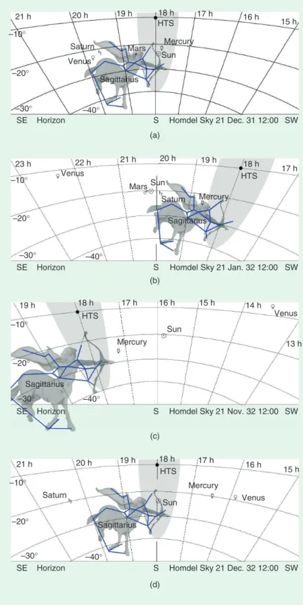
It is interesting to have a pictorial view of the sky seen by Jansky at the Holmdel site at some periods during his experiment. In Figure 8, four sky maps, focusing on times and regions of inter-est, are given to better appreciate the motion of the Sagittarius constellation with respect to the sun: on a monthly scale, by comparing Figure 8(a) with (b), and (c) with (d); on a yearly scale, by comparing the first two maps with the last two. It is interesting also to notice, highlighted in every map, the HTS posi-tion and the antenna pointing error as estimated by Jansky.

Jansky described his results in tech-nical [4] and popular [5] papers, both fundamental to the birth of radio astron-omy: it was after reading those papers that Grote Reber became increasingly fascinated with celestial radio emission, 18 12 6 18 12 6 18 12 6 18 12 6 12:00 p.m. 1:00 p.m. 2:00 p.m. 3:00 p.m. 3:00 p.m. 4:00 p.m. 5:00 p.m. 6:00 p.m. 6:00 p.m. 7:00 p.m. 8:00 p.m. 9:00 p.m. 9:00 p.m. 10:00 p.m. 11:00 p.m. 12:00 a.m. Relative Intensity (dB) N W S E N W S E N W S E N W S E N W S E N W S E N W S E N W S E NW S EN 16 Sept. 1932

FIGURE 6.

A daytime record of the mysterious hiss-type signal from September 1932.

The 20-min periodicity of the antenna azimuth rotation is evident.

1) 21 Jan. 1932 5) 8 May 1932 2) 24 Feb. 1932 6) 11 June 1932 3) 4 Mar. 1932 7) 15 July 1932 4) 9 Apr. 1932 8) 21 Aug. 1932 9) 17 Sept. 1932 10) 8 Oct. 1932 11) 4 Dec. 1932 N 180° N 180° W 90° E 270° S 0°

Azimuth of the Direction of Arrival

12:00

a.m. 4:00a.m. 8:00a.m. 12:00p.m. 4:00p.m. 8:00p.m. 12:00a.m. 0 2 4 Time of Day

Intensity (dB) Above Set Noise

2 1 ₁₁ 10 9 8 7 6 5 4 3 2 1 11 10 9 8 7 6 5 5 4 4

FIGURE 7.

A graph of the azimuth of the direction of arrival of hiss-type waves plotted

against time of day.

Jansky concluded that

the hiss-type source was

synchronous with sidereal

time, not solar time, thus

being fixed in the sky in

the same fashion as are

all the stars.

built the very first radio telescope to pur-posely make a radio map of the Milky Way, and took the second step in the development of radio astronomy.

JANSKY’S ANTENNA

The ba sic element of t he Ja nsk y merry-go-round was a Bruce-type array [6], developed shortly before the Jansky experiments by Edmond Bruce (a U.S. radio engineer) for transoceanic radio communications when Bruce was working in the group of Harald Trap Friis (a Danish radio engineer) at Bell Laboratories. The Bruce array is a vertically polar-ized broadside array, which Jansky used as both active monopole ele-ment and as passive reflector over a bandwidth of about 26 kHz centered at about 20.5 MHz. Each element was made of 7/8-in brass pipes, sup-ported by glass insulators on a fir lumber frame (Figure 3). The active array element (Figure 9) was a four-period, half-wavelength-amplitude square-wave, with one-half duty cycle and half-wavelength period width, starting (and terminating) with an open-ended, eighth-wave-length-long, low-level section. The passive element was almost identical to the active element, except 15% taller and separated by one-quarter wavelength.

At the design frequency, the part of the antenna concerned with radiation is limited to the vertical wires only, where standing wave currents oscillate in phase. The presence of the passive array makes the antenna beam pattern unidirectional, in the direction from the passive to the active element. The earth below the antenna behaves like a ground plane, and the effect is to raise the main beam above the horizontal plane. Those were exactly the ideal fea-tures for a receiving antenna scanning for static on a ground-based platform, as already discussed. Today, about 85 years after Jansky’s experiment, due to the availability of electromagnetic software packages and highly efficient computer hardware, it is possible to carry out a sort of time-reversed engi-neering and simulate the performance

21 h 23 h 22 h 21 h 20 h 19 h 19 h 19 h 21 h 20 h 18 h 18 h 18 h 17 h 17 h 17 h 16 h 16 h 15 h 15 h 14 h 13 h HTS HTS HTS 20 h 19 h 18 h 17 h 16 h _{15 h} HTS –10° –10° –10° –10° –20° –20° –20° –20° –30° –30° –30° –30° –40° –40° –40° –40° Saturn Saturn Venus Venus Venus Venus Mars Mars Sun Sun Sun Sun Mercury Mercury Mercury Mercury Sagittarius Sagittarius Sagittarius Sagittarius

SE Horizon S Homdel Sky 21 Dec. 31 12:00 SW

SE Horizon S Homdel Sky 21 Jan. 32 12:00 SW

SE Horizon S Homdel Sky 21 Nov. 32 12:00 SW

SE Horizon S Homdel Sky 21 Dec. 32 12:00 SW Saturn

(a)

(b)

(c)

(d)

FIGURE 8.

Holmdel sky maps centered on the south (S) direction and taken at

noon on some particular days during the Jansky experiments. Maps (a) and (b) are from the beginning and (c) and (d) from the end of the year-long experiment. The positions of planets, the sun, and the Sagittarius constellation are indicated on the equatorial grid giving right ascension and declination. The HTS position, as estimated by Jansky, is centered on the HPBW spot of the Jansky antenna. SE: southeast; SW: southwest.

114 A U G U S T 2 0 1 9 IEEE ANTENNAS & PROPAGATION MAGAZINE of an accurate electromagnetic model of Jansky’s antenna.

The Bruce array is basically a wire antenna, and method of moments (MoM)-based software [7], [8] is able to accurately characterize the current distri-bution in the wires, taking into account the effects of finite wire diameter. Also, the effect of the earth, modeled in the simulations by a circular four-wavelength-diameter perfect electric conductor ground plane, can be taken into account. Finally, a voltage source placed from the center of the active element to the ground is used to excite the antenna.

The electromagnetic model and some analysis data at 20.5 MHz are given in Figure 10. The simulated cur-rent distribution is superimposed on the wires, and, from the arrow direc-tions, phase matching on the verti-cal wires can be clearly observed. A 3D pattern with a maximum above-the-ground level in the positive x-axis direction (Figure 10) is also plotted and superimposed on the geometry.

A more precise characterization of the antenna beam at 20.5 MHz is given in the beam principal plane cuts, plot-ted in Figure 11. Jansky’s antenna has a directivity of about 15 dBi, a HPBW of about 24º in the azimuth plane (H-plane) and about 30º in the eleva-tion plane (E-plane). The direceleva-tion of the maximum in the elevation plane is about 30º above the horizon. Variables

{ and j used in the polar plots in Fig-ure 11 correspond to the angular coor-dinates of a spherical system referenced to the x, y, and z axes in Figure 10.

The MoM numerical model also allows us to characterize the input

λ /8 λ /4

λ /4

λ /2

Feeding Point

FIGURE 9.

A sketch of the active element of the Jansky merry-go-round antenna. In

evidence are the period and the feeding point.

x

y z

FIGURE 10.

An electromagnetic model of the Bruce-type array used by Jansky

obtained using the FEKO software package. The current peak distribution along the wires and the antenna 3D radiation pattern are shown.

0° 0° 270° 270° 180° 180° 90° 90° 15 dBi 15 dBi 12 12 9 9 6 6 3 –3 0 3 –3 0 ϑ φ (a) (b)

FIGURE 11.

Polar plots of the principal plane cuts of Jansky’s antenna. (a) E-plane

(elevation) and (b) H-plane (azimuth).

0 –5 –10 –15 –20 S11 (dB) 16 17 18 19 20 21 22 23 Frequency (MHz)

FIGURE 12.

A graph of the input matching

matching of the Jansky antenna. Using a 50-Ω reference impedance, the simulated input matching over a quite broad band (16–23 MHz), including the Jansky-exper-iment central-frequency of 20.5 MHz, is plotted in Figure 12. The simulation shows a –10 dB reflection coefficient bandwidth of about 3.5 MHz (18–21.5 MHz).

AUTHOR INFORMATION

Renzo Nesti (renzo.nesti@inaf.it) is with

the Italian National Institute for Astro-physics at the Arcetri Astrophysical Observatory, Florence. His research interests are in the area of antennas and

microwave devices for radio astronomy receivers, including numerical methods for electromagnetic analysis and design.

REFERENCES

[1] W. T. Sullivan III, The Early Years of Radio Astron-omy: Reflections Fifty Years After Jansky’s Discovery. Cambridge, UK: Cambridge Univ. Press, 1984. [2] W. A. Imbriale, “Introduction to ‘electrical disturbances apparently of extraterrestrial origin,’” Proc. IEEE, vol. 86, no. 7, pp. 1507–1509, July 1998. doi: 10.1109/JPROC.1998.681377.

[3] K. G. Jansky, “Directional studies of atmo-spherics at high frequencies,” Proc. IRE, vol. 20, no. 12, pp. 1920–1932, Dec. 1932. doi: 10.1109/ JRPROC.1932.227477.

[4] K. G. Jansky, “Electrical disturbances appar-ently of extraterrestrial origin,” Proc. IRE, vol. 21,

no. 10, pp. 1387–1398, Oct. 1933. doi: 10.1109/ JRPROC.1933.227458.

[5] K. G. Jansky, “Radio waves from outside the solar system,” Nature, vol. 132, no. 3323, pp. 66, July 1933. doi: 10.1038/132066a0.

[6] A. A. Oswald, “Transoceanic telephone service—Short-wave equipment,” Trans. AIEE, vol. 49, no. 2, pp. 629–637, Apr. 1930. doi: 10.1109/ T-AIEE.1930.5055547.

[7] G. J. Burke and A. J. Poggio, “Numerical elec-tromagnetics code (NEC)—Method of moments,” U.S. Naval Ocean Systems Center, San Diego, CA, Rep. NOSC-TD116-vol 1, 1981. [Online]. Available: https://apps.dtic.mil/dtic/tr/fulltext/u2/ a956129.pdf

[8] Altair HyperWorks, “Altair FEKO,” 2018. [Online]. Available: https://altairhyperworks.com/ product/Feko

SHARE AND MANAGE

YOUR RESEARCH DATA

IEEE DataPort is an accessible online platform that enables researchers

to easily share, access, and manage datasets in one trusted location.

The platform accepts all types of datasets, up to 2TB, and dataset

up-loads are currently free of charge.