Macroeconomic factors and small bank failures: the case of the italian cooperative banks

Contents

ACKNOWLEDGMENTS ... I

1 INTRODUCTION ... 1

2 AIM AND MOTIVATION ... 3

3 LITERATURE REVIEW ... 5

4 THE INTERNATIONAL FINANCIAL CRISIS AND BANKING SYSTEMIC RISK ... 11

5 THE ITALIAN COOPERATIVE BANKS: AN OVERVIEW... 14

6 METHOD ... 19

6.1Model description ... 19

6.1.1Pooled cross section regression ... 22

6.1.2Unobserved effects models ... 23

6.1.3Lag structure ... 26

6.1.4Test for the contribution of macroeconomic factors ... 27

6.2Sample and data sources ... 28

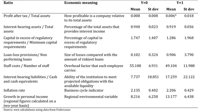
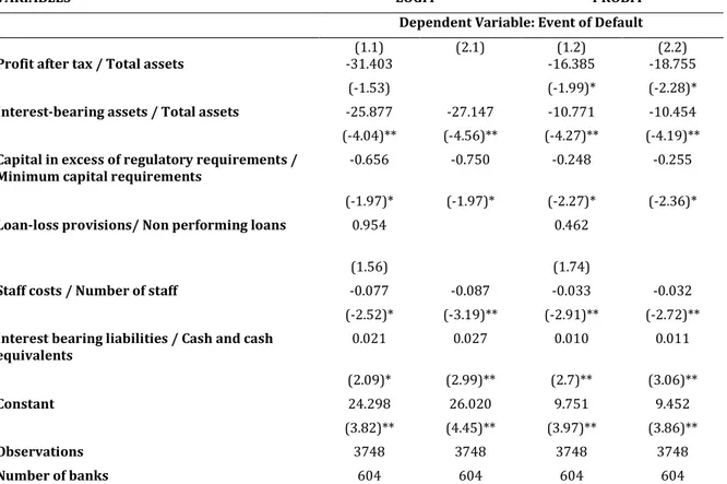
6.3Definition of failure ... 31 6.4Input variables ... 33 6.4.1Subset selection ... 34 6.4.2Explanatory variables ... 36 7 RESULTS ... 38 7.1In-sample performance ... 46 7.2Robustness test ... 49 8 CONCLUSIONS ... 53 9 REFERENCES ... 55 10 APPENDIX ... 61

ACKNOWLEDGMENTS

By the end of such exciting journey, different are the feelings. From one hand, it is easy to look back and see how much you have done in these years. From the very beginning until today, there is so much progress that you cannot believe how many millions miles you have walked. On the other hand, the future is in front of you and you know that new challenges are in the immediate upcoming days. Thus, my luggage is already ready.

First of all, I want to tank my parents and my sister for their stunning support. I see them always by my side and I feel they participate actively in my work. Secondly, I feel extremely grateful to Franco Fiordelisi for his support and patience. The guidance and wise expertise of my tutor made things easier to understand and it motivates and stimulates my research activities. Through your collaboration I have grown as a researcher and as a person. Many thanks and I hope we will have the opportunity to work together in the future.

Another special thank is to Maria Paula and the people from Barcelona GSE. Maria Paula has been revising my PhD thesis hundreds of times and through our conversations, I had the opportunity to understand the deep implications of my research. The people from BGSE give me the possibility to have different perspectives and insights on my research topic. In particular, thanks to Andrea Petrella, I understood the technical issues related to the method employed in the analysis.

I would also like to express my special thank to Gianluca Mattarocci for his useful help. In addition, I would like to thank the faculty member, the PhD coordinator Professor Alessandro Carretta, Professor Previati and David Pelilli. All of you have made possible the realization of this research work.

Finally, least but not last, I would like to tank Federcasse for providing me with the data necessary for the estimation of the model and for the helpful collaboration, especially in the persons of Alessandra Appennini and Roberto Di Salvo.

My last thought is to my friends Giacomo, Enrico and Tiziana, to Isabella who witnessed the onset of this hard journey, and to all the nice people that have follow me in this vibrating experience. Without you, it would have been impossible reaching the end.

1 INTRODUCTION

The recent financial turmoil has renewed the attention of governments and financial authorities on the endemic risks associated to banking operations. The reluctance of banks to lend to each other together with less liquid financial markets has brought to an increase in the number of failures of financial institutions. As a consequence, it is of utmost importance to further explore the banks' exposure to credit risk.

The research presents an innovative study related to the analysis of the determinants of risk of failure for small banks. The investigation clarifies the relationship between the specific characteristics of small banks and their probability of failure. The issue is of particular relevance for the socio-economic role of this type of financial institutions and for the lack of the research on the subject. Thus, the present analysis develops a default predictive model using the panel data technique.

This study focuses on small banks for two main reasons. First, these banks play an important role at a local and national level. For instance, European cooperative banks serve more than 176 million clients, manage over EUR 5 trillion in assets and hold a deposits and credits market share of 21% and 19% respectively1

. Second, a few studies provide a comprehensive picture of the main determinants of risk for small banks. In particular, there is a little knowledge about the relationship between their probability of default2

and the local economic conditions.

From a theoretical point of view, banks are affected by the economy in which they do business. The relevant economic conditions for small banks are local due to the limited geographic market and legal restrictions. Cooperative model - as a distinct business model - exposes the banks to the cyclical fluctuations of the national and local economy3_. Hence, I explore whether nonbank economic data can be used to improve forecasts of small bank health.

1

Source of data: European Association of Cooperative Banks (EACB), key statistics as on 31-12-2008. 2

In this study the term default will, except where otherwise noted, refer to the definition adopted in the estimation of the model (see §6.3).

3

The analysis employs the panel data technique to show that cooperative failures prediction is statistically related to macroeconomic variables and bank-level fundamentals. The focus is on Italian cooperative banks (CB)4 _{since this case is} particularly interesting to analyze the interconnection between small banks and the local economic environment. Hence the study shows that the inflation rate and the growth in personal income are statistically significant and affects positively the probability of default. As a result, this finding will contribute to the growing literature of explaining the causes of bank failures and it will allow formulating related policies in order to head off the potential crisis or limit its direct and indirect costs.

The remainder of the paper is organized as follows. Section 2 introduces the aim and motivation of the research. Section 3 briefly reviews the relevant literature. Section 4 provides a concise overview on the recent financial crisis and it highlights the relevant issues related with the present investigation. Section 5 describes the Italian Cooperative banking sector. Section 6 deals with the method, the data used for the estimation and provides a description of the procedure utilized for the model specification. Section 7 details the results of the analysis and Section 8 concludes.

4

For the sake of simplicity, the term “Italian Cooperative Banks” or “Cooperatives” or “CB” stands for: 1. Banche di credito cooperativo;

2. Casse rurali; 3. Casse Raiffeisen.

2 AIM AND MOTIVATION

Banks are key financial institutions for the functioning of financial markets. Moreover, there are several reasons why regulating the banking sector is of utmost importance. First, the maintenance of good level of confidence prevents the adverse effects of bank runs on the economy. Second, there is official concern about systemic risk in the banking sector and the possibility of a chain reaction of bank defaults (domino effect). Multiple bank failures might precipitate a sudden contraction of the money supply and severely disrupt the real economy5

. Third, bank failures can disrupt the flow of credit to local communities. To the extent that these events are socially inefficient, public intervention may be justified6_.

The recent financial crisis has demonstrated how economic units have become more internationally linked to each other. As a consequence, deterioration in the financial health of one institution could lead to the domino effect. It seems then surprising that not much work has been done regarding the assessment of small bank’s risk of failure. For instance, European cooperative banks represent a pretty homogeneous sample that could be analyzed in order to fulfil the apparent lack of research in this field. Moreover, the intrinsic characteristics of the European cooperative banks give room to a further investigation on the deep ties between the economic environment and bank performances. In this regard, it is important to remark that there is a clear difference between the small retail business banking (the majority of cooperative banks especially in Italy, Austria and Germany) and big cooperative networks that have expanded their operations beyond their domestic markets (i.e. Crédit Agricole and Rabobank). In fact, small banks are more exposed to the influences of the local environment due to the type of their business model. Then, an appropriate sample selection should be done to detect the banks that are more suitable for the analysis. To this end, this research represents a first step toward this goal. By examining the Italian cooperative banks, it is possible to detect the main drivers of risk that affects small bank failures. Additionally, Italian cooperatives are unquestionably local banks and represent a homogeneous sample due to legal restrictions and to their business operation model. Furthermore, since it is

5

Dale (1984). 6

particular high the information asymmetry between this type of banks and outside analysts, the study provides a useful insight on Italian cooperative banking system and contributes to understand under what conditions the relationship between the economic environment and the bank risk of default become significant.

The case of Italian cooperative banking is particularly interesting for various reasons. First, CBs represent a systemic threat to the safety and soundness of the domestic banking system (deposits and credits market share of 8.9% and 7.2% respectively7

). Second, as already noted by Goodhart (2004), the presence of any non-profit-maximizing banking entities may make financial systems more fragile. In this regard, CBs are more susceptible to failure since are less able to diversify8

. Third, Italy displays a geographical diversity that need to be considered to accurately estimate the bankruptcy probability. In fact, the Italian case is particular interesting since the presence of many local systems and marked territorial imbalances in levels of development represents a significant laboratory to analyze empirically the effect of macroeconomic factors on the individual bank probability of default. Fourth, the number of the ceased banks analyzed in the sample was quite large (i.e. 34 cases).

The purpose of the research is to estimate the probability of default of Italian cooperative banks by using a comprehensive set of information. By using an econometric model is possible to draw some inference from the data about any relationships that might exist between bank failures and some characteristics. This instrument may be also useful to pinpoint the source of developing problems and to understand the evolution of banking operations and the banks’ risk exposure. Furthermore, it helps to introduce control variables that capture the heterogeneity between banks located in different geographical areas. As a consequence, the different conditions displayed by the Italian country regions are proxied by the growth in personal income.

7

Source of data: European Association of Cooperative Banks (EACB), key statistics as on 31-12-2008. 8

The study from Wheelock and Wilson (2000) demonstrates that an ability to create a branch networks, and an associated ability to diversify, reduces banks’ probability of failure.

3 LITERATURE REVIEW

Although there are a handful of studies on bank failures and banking crisis, there seem to be two separate streams in the empirical literature9

: the “micro” and the “macro” camps. The “micro” approach focuses in general on individual banks’ balance sheet data, possibly augmented with market data, to predict bank failure. The “macro” approach explains the banking crises examining the macroeconomic determinants. These studies typically analyze a large sample of countries trying to find out which macroeconomic variables signal the happening of a banking crisis in advance. Several works have been done in both areas but a few have tried to combine the two approaches together.

Bankruptcy predictions aiming at detecting individual failures using financial ratios have become important research topics after the pioneeristic research of Altman (1968) and Beaver (1966). These studies try to discriminate between sound and unsound institutions using accounting data. Soon after their introduction, several studies test the predictive ability of financial ratios to detect the financial health of bank operations.

Among the statistical techniques analyzing and predicting bank failures, discriminant analysis10

and the method of multiple regression have been the most employed for many years. Meyer and Pifer (1970) develop a qualitative response model on impaired U.S. banks. The authors perform a cross-sectional regression using financial variables and qualitative measures related to trends, variation and unexpected changes. Subsequent work by Sinkey (1975) and Santomero and Visno (1977) also focus on the U.S. banking market and draw mainly on discriminant analysis for the classification of banks. The former study uses a multiple discriminant analysis11

of the balance-sheet and income-statement of problem banks to identify financial characteristics which distinguish between the two groups (problem and non-problem banks), whilst the latter research

9

Gonzalez-Hermosillo (1999). 10

To its bare essentials, this technique looks for a function that maximizes the ratio of among-group to within-group variability, assuming that the variables follow a multivariate normal distribution and that the dispersion matrices of the groups are equal. There are three main subcategories of discriminant analysis: linear, multivariate and quadratic. 11

The basic assumptions of the technique, as described in Sinkey (1975) are: 1. the groups being investigated are discrete and identifiable;

2. each observation in each group can be described by a vector of m variables or characteristics; 3. these m variables are assumed to have a multivariate normal distribution in each population.

focuses on the estimation of cross-section failure probabilities for the American commercial banking system using a stochastic process technique.

As generally financial ratios are not normally distributed12

, maximum-likelihood methods13

have been employed more frequently. Martin (1977) performs a comparison between logit and discriminant models. The dependent variable is the occurrence of failure of the U.S. commercial banks whilst various combinations of financial ratios are utilized as independent variables. Espahbodi (1991) argues that logit model would be more appropriate than discriminant analysis for development of binary choice models as it is theoretically superior. In addition, the author tests that logit model performs at least as well as discriminant analysis. West (1985) uses a factor analysis/logit approach for identifying problem banks. The author first run a factor analysis to detect the common characteristics that influence the conditions of banks, then tests their ability to distinguish problem from sound banks. The statistic employed in the second step is a maximum-likelihood logit regression with the factor scores as variables. Logan (2001) implements a logit model to identify leading indicators of failure for U.K. small banks. The analysis focuses on a particular episode (small banks’ crisis of the early 1990s in U.K.), though it gives a compelling insight on the main drivers of risk characterizing the small and medium sized banks.

Other techniques have been employed later in order to generate estimates of the probability of bank failure or, alternatively, of bank survival. The advantage consists in the possibility of determining the probable time of failure and in obtaining time-varying covariates. Lane et al. (1986) pioneered the field by using duration analysis. The authors were first in applying the Cox proportional hazards model14

to the prediction of US commercial bank failures. Estrella et al. (2000) estimate the likelihood of failure using

12

Eisenbeis (1977). Violations of the normality assumptions may bias the test of significance and estimated error rates.

13

Essentially, the maximum-likelihood technique is used for fitting a mathematical model to data. It implies the use of differential calculus to determine the maximum of the probability function of a number of sample parameters (for example the mean and the variance). The moments method equates values of sample moments (functions describing the parameter) to population moments. The solution of the equation gives the desired estimate.

14

This method produces estimates of the probability that a bank with a given set of characteristics will survive longer than some specified length of time into the future (Whalen, 1991). An important issue of the hazard models is that it is possible to incorporate macroeconomic variables whose value is unique for all firms at a given point in time.

cross-sectional logit regressions and then analyze the time-dependency in the conditional probability of failure through a proportional hazard model. Glennon et al. (2002) employ a parametric method of logit analysis and a nonparametric approach of trait recognition15

. The authors analyze a sample of large U.S. banks comparing both techniques. Although both methods perform well in the classification results of original samples, trait recognition outperformed logit in terms of minimizing Type I errors (i.e., identifying a failed bank as nonfailing) and Type II errors16

(i.e., identifying a nonfailed bank as failing) using holdout samples. Wheelock and Wilson (2000) use a competing-risks hazard model to identifying characteristics leading to either failure or acquisition. The authors demonstrate that US banks with lower capitalization, highly-leveraged, lower liquidity, poor quality loan portfolios and lower earnings are more prone to failure. Moreover, they find that banks located in state where branching is permitted are less likely to fail, indicating the benefits of geographic diversification. Shumway (2001) develop a discrete-time hazard model to determine probability estimates for all firms at each point in time. The author argues that hazard models are theoretically preferable to single-period classification models (static model) since they consider that firms change over and through the time. Hence the resultant probabilities of default approximate consistently the true probabilities of failure. Canbas et al. (2005) propose an integrated early warning system (IEWS) for Turkish commercial banks. The authors use the principal component analysis17

to select the relevant financial factors and then estimate discriminant, logit and probit models based on these characteristics. Lanine and Vennet (2006) employ a parametric logit model and a nonparametric trait recognition approach

15

Glennon et al. (2002) provided a general description of trait recognition. The nonparametric approach consists in a multi-step procedure:

1. selecting cutpoints for each of the variables; 2. binary coding of the variables;

3. constructing a trait matrix for each observation; 4. identifying good and bad traits (or distinctive features); 5. implementing voting matrix classification rules. 16

Type 1 error and Type 2 error are related to hypothesis testing. Type 1 error arises when the test rejects the null hypothesis when the null hypothesis is true (false positive); Type 2 error occurs when it fails to reject the null hypothesis when the null hypothesis is false (false negative).

17

Principal component analysis (PCA) is a statistical method that can be used to reduce the dimension in multivariate analysis.

to predict failures among Russian commercial banks. The study tests if bank-specific characteristics can be used to predict vulnerability to failures and it shows that liquidity, asset quality and capital adequacy were important determinants of bankruptcy.

The most recent methods use the latest developments in intelligence techniques. The main advantages are that the models do not make assumptions about the statistical distribution or properties of the data and that intelligence technique rely on nonlinear approaches. Among these methods, neural networks are the most widely used18

. Boyacioglu et al. (2009) propose a comparison between various neural network techniques (NN), support vector machines (SVMs) and multivariate statistical methods19

. The methods are applied to bank failure prediction problem in the Turkish case. Neural networks and in particular the multi-layer perception (MLP) and the learning vector quantization (LVQ), are found to be the most effective techniques in predicting the bank failures in the sample. Ioannidis et al. (2010) model bank soundness at individual bank level using an innovative set of explanatory variables and various classification methods belonging both to statistical and artificial intelligent techniques. The authors investigate first the classification accuracy of models that include bank-level data only with those that include a full set of variable (financial ratio, regulatory variables and other country-level variables), then propose an integrated model to test if model combination increases the classification accuracy. The best two models in terms of the average classification accuracy are developed with UTADIS20

and artificial neural networks. In addition, the study finds that the use of country-level variable significantly improve the classification accuracies of the models.

The usage of macroeconomic information in default predicting models is still under debate. Several works21

have attempted to determine if and under which conditions environmental influences affect banks’ likelihood of failure. Just a few of those studies have introduced some macroeconomic/regional factors as explanatory variables for

18

Boyacioglu et al. (2009). This technique mimics the learning process of the human brain. Through several constructs and algorithms, the system has the ability to learn from examples and to adapt to new situations.

19

See Boyacioglu et al. (2009) for an extensive explanation of the techniques employed. 20

This approach uses an additive utility function to score the banks and decide upon their classification. 21

individual bank failures. For instance, Nuxoll (2003) uses a logistic model22 to demonstrate that state-level economic variables do not improve the forecasts of US bank health. The model assumes a two-year horizon and combines economic information (personal-income data, employment data, and banking aggregates) with Call Report and examination data. On the other hand, Porath (2006) finds that macroeconomic information significantly improves default forecasts in the case of German savings banks and credit cooperatives. Using a panel binary response model, the author shows that including macroeconomic variables such capital market, interest rate and firm insolvencies, improve default forecasts. Furthermore, studies that look at the banking system as a whole often employ a heterogeneous set of control variables. Demirguc-Kunt and Detragiache (1998) use a multivariate logit model to examine the determinants of the probability of a banking crisis around the world in the period 1980-1994. The research underlines that elements of the macroeconomic environment, such GDP growth, excessively high real interest rates and high inflation, significantly increase the likelihood of systemic banking crises. Davis and Karim (2008) assess the multivariate logit model and the signal extraction model for banking crises. The model is run on a panel of 105 countries and it uses Demirguc-Kunt and Detragiache (1998) variables to show that the parametric approach may be better suited to global Early Warning Systems23

(EWS) whereas the non-parametric approach may be better suited to country-specific EWS. Gonzalez-Hermosillo (1999) analyzes the role of both micro and macro factors in the occurrence of banking system distress in the United States, Mexico and Colombia in the 1980s and 1990s. Using a fixed-effects logit for panel data and a survival time model, the author argues that bank-specific variables seem to capture the fundamental sources of ex-ante risk. Then, the introduction of the macroeconomic or regional variables enhances the predictive power of the models based on bank-specific data only. Arena (2008) performs both cross-sectional logit estimation and survival time analysis to prove that bank-level fundamentals, banking system and macroeconomic variables significantly affect the likelihood of bank failures in the case of banking crises in East Asia and Latin America. In addition, the author suggests that systemic macroeconomic and liquidity

22

The model was estimated both as a cross section and as a pooled time-series cross section. 23

Systems that assist supervisors and examiners in identifying changes, particularly deterioration, in banks’ financial condition as early as possible.

shocks not only destabilize the banks that were already weak before the crises, but also the relatively stronger banks ex-ante. This result suggests that even strong banks can be particularly affected by the negative effects triggered by systemic crises.

A few studies have assessed the probability of default of the Italian cooperative banks. The most recent work has been carried out by Guidi (2005). The author develops an early-warning system expressing the probability of future failure as a function of accounting ratios. The statistical method employed is a logistic analysis using five weighted samples of sound and problem banks24_{. The empirical findings indicate that} banking factors25

such liquidity, efficiency, profitability, capital adequacy, credit risk exposure and asset and deposit compositions are good discriminators between the groups and, in particular, profitability and risk profile are of great importance. Nevertheless, the study does not take directly into consideration the explicit influence of the macroeconomic environment on bank operations. Moreover, it does not analyze the time-variant relationship existing between the set of characteristics used and the occurrence of bank default. These features give room to the present research, also on the light of the systemic threat represented by the failure of individual banks.

24

The problem banks represent the group of observation that goes into crisis within one, two and three years of the statement year to which accounting ratio data apply.

25

4 THE INTERNATIONAL FINANCIAL CRISIS AND BANKING SYSTEMIC RISK

This section briefly reports the main facts of the financial turmoil started in 2007. The recent maelstrom demonstrates that bank failures threaten the economic system as a whole. The severe instability experienced by the banking system has deeply affected real economies of many countries in the world causing recessions, the burst of the housing bubble and a relentless global credit crunch. Thus, the description of the mechanisms at work may be of help in understanding the importance of evaluating the soundness of individual banks. In addition, it would be useful in underling some of the characteristics that may be important in preventing the occurrence of small bank default.

The US subprime market witnessed the onset of the crisis. Different were the main causes of the collapse. A first key signal was the significant increase in the delinquency and foreclosure rates for mortgages originated in 2006 and 2007. The quality of loans had started to decline since year 200126

but this feature came to light when the housing prices started declining. Securitization definitely triggered this process since it adversely affected the screening incentives. It brought a change in bank operation model from originate-to-hold to originate-to-distribute and it reduced the incentives of financial intermediaries to screen borrowers. In addition, the ease monetary policy between 2002-2004 led to the housing boom and its subsequent collapse. Another related fact is that subprime mortgages were temporary phenomenon27

, i.e. the main scope to sign a mortgage was either to speculate on house prices or to improve customer credit history. Demyanyk (2008) shows in fact that approximately 80% of borrowers either prepaid or defaulted on mortgage contracts within 3 years of mortgage origination. All this, join with the overall economic slowdown, generates the market collapse. What is more, the close ties between financial institutions generate a spread of the crisis beyond US boundaries and a global credit crunch.

The large effect of the relatively small subprime component of the mortgage market poses interesting questions about the banking systemic risk. The complexity of the securities created by pooling individual subprime mortgages together, made difficult valuing the holding of such complicated financial instruments. Moreover, the complex

26

Demyanyk and Hasan (2010). 27

financial process were characterised by highly leveraged borrowing, inadequate risk analysis and limited regulation. In particular, financial liberalisation provided another source of systemic risks, as well-documented by several studies28_{. All this ultimately} resulted in uncertainty that worsen the asymmetric information problem. Furthermore, since the securities were largely traded internationally, when the fears related to the declining of the US housing market spread across the financial markets, the complex web of financial innovations that had purportedly been employed to reduce risk prompted the crisis spread across the financial markets and into the real economy. The crisis hit the broader banking industry and the growing counterparty risk further tightened credit channels generating a self-sustaining loop.

Banking systemic risk reflects a correlation of performance between institutions29 . One possibility is that such crises materialise through individual liquidity failures of solvent banks that become contagious. In this regard the analysis of the Italian cooperative banks can lessen the asymmetric problem and limit the effects of the associated bank runs. The role of confidence in precipitating runs is emphasised in Diamond and Dybvig (1983). Whenever panic spread across investors, a bank’s underlying position is almost irrelevant and individual bank failure may spread through contagion associated with asymmetric information. Another characteristic that is also of utmost importance in the analysis of cooperative model is the direct financial exposures that tie together this type of banks. As it will be shown in the next sections, Italian cooperative banks are deeply interrelated between each other and the counterparty claims between them may lead to widespread failures30

. In addition, since Italian cooperative banks are key players in the domestic market, the systemic risk is sufficiently deep for a crisis to be triggered.

In conclusion, a succession of bankruptcies around the world and the rescue of apparently rock-solid banks and insurance companies have left millions of worldwide citizens in a state of anxiety and concern. Bank supervisors are called to preserve the stability of the financial system favouring sound banking. One first step, at least in Italy, would be having a clearer idea of the determinants of risk of cooperative banks. This

28

Among the other studies, Kaminsky and Reinhart (1999), Demirguc-Kunt and Detragiache (1998). 29

Davis, Karim (2008). 30

would be of help in limiting the effects of the endogenous risks associated with this type of banks and in increasing the knowledge and the available information regarding key nationally financial players.

5 THE ITALIAN COOPERATIVE BANKS: AN OVERVIEW

Cooperative banks represent a valuable addition to the Italian banking sector. Furthermore, these banks are local institutions and constitute a direct link between market, small enterprises, and citizens. Through their widespread presence on national territory, they are the driving forces and actors of regional and local development. Moreover, CBs contribute to the competitiveness and stability of the Italian banking industry, though the cooperative model is very much different to the commercial banking model.

Cooperative banks are peculiar for their intrinsic features and are subject to specific regulations. According to the 1993 Banking Law, CBs shall grant credit primarily to their member31

(mutual ends). Moreover, they have a restriction to geographical expansion32 and shares are non-tradable since they do not reflect the value of the firm because profits are mostly devoted to a reserve fund33

. Decision making is based on the one-person-one-vote principle34_{. This leads to conservative risk management and to enhanced trust} between the local cooperative bank and its members/customers. In addition, ownership rights are limited to ensure that contributions are similar.

The Italian cooperatives are fully autonomous in their decisions but cooperate intensively through network institutions. They are grouped into 15 regional federations, which report to Federcasse, the national association. The regional federations provide technical assistance and internal auditing to their members, whilst the national association is in charge of the strategic planning and institutional affairs; more specifically, the national association sets strategic policy guidelines for cooperative banking with the aim of achieving ethical, cultural, social and economic objectives. Similarly, specialist products are created through consortium-structured initiatives. In addition, a “safety net” guarantees the going-concern basis: CBs’ deposits and bonds are covered by two specific guarantee funds (Fondo Garanzia Depositanti and Fondo

31

Banking law (Art. 35). At least 50% of risky assets should relate to transactions with members. 32

Banking law (Art. 35). At least 95% of risky assets should relate to transactions in the geographic area of competence.

33

At least 70% of the annual net profits must be allocated to the legal reserve fund. 34

Garanzia Obbligazionisti), whilst the other liabilities are guaranteed by the “Fondo di Garanzia Istituzionale Tutela globale per il risparmiatore cliente delle BCC”. Moreover, through Federcasse, CBs are internationally represented by the European Association of Cooperative Banks (EACB), based in Brussels.

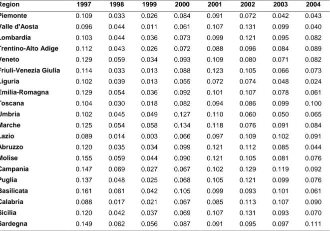
The structure of the sector reflects the evident regional orientation of this type of banks. For this reason, the analysis of the influence of the economic environment is of interest. Furthermore, the geographical restrictions make bank operations prevalently oriented to the local area, diminishing the possibility for a geographical diversification. Additionally, the Italian regions display a very different social, economic and topographic condition that should be considered in the analysis of CBs possible exposure at risk. For instance, the distribution of the growth in personal income calculated over a two year period shows a marked difference (on average) between northern and southern regions.

Table 1: “Distribution of two-year growth in personal income by year and region”

Region 1997 1998 1999 2000 2001 2002 2003 2004 Piemonte 0.109 0.033 0.026 0.084 0.091 0.072 0.042 0.043 Valle d'Aosta 0.096 0.044 0.011 0.061 0.107 0.131 0.099 0.040 Lombardia 0.103 0.044 0.036 0.073 0.099 0.121 0.095 0.082 Trentino-Alto Adige 0.112 0.043 0.026 0.072 0.088 0.096 0.084 0.089 Veneto 0.129 0.059 0.034 0.093 0.109 0.080 0.071 0.082 Friuli-Venezia Giulia 0.114 0.033 0.013 0.088 0.123 0.105 0.066 0.073 Liguria 0.102 0.039 0.013 0.055 0.072 0.074 0.048 0.024 Emilia-Romagna 0.129 0.054 0.036 0.092 0.101 0.107 0.078 0.061 Toscana 0.104 0.030 0.018 0.082 0.094 0.086 0.099 0.100 Umbria 0.102 0.045 0.049 0.127 0.110 0.060 0.050 0.065 Marche 0.125 0.054 0.058 0.134 0.118 0.076 0.091 0.084 Lazio 0.089 0.014 0.003 0.066 0.097 0.109 0.102 0.091 Abruzzo 0.120 0.035 0.034 0.099 0.121 0.112 0.085 0.044 Molise 0.155 0.059 0.044 0.090 0.121 0.105 0.081 0.076 Campania 0.147 0.069 0.027 0.067 0.102 0.129 0.119 0.092 Puglia 0.137 0.048 0.025 0.068 0.105 0.121 0.099 0.076 Basilicata 0.161 0.061 0.042 0.105 0.099 0.093 0.101 0.061 Calabria 0.088 0.017 0.021 0.067 0.085 0.113 0.107 0.090 Sicilia 0.120 0.042 0.037 0.069 0.107 0.131 0.093 0.070 Sardegna 0.149 0.062 0.056 0.087 0.091 0.095 0.097 0.111

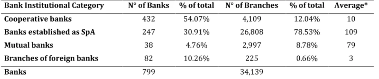
The Italian banking sector comprises 799 banks, of which almost 54% are cooperative banks. The sector also includes joint stock companies (SpA), foreign banks and another

type of entity operating under a cooperative structure (mutual banks)35

. CBs account for almost 12% of all retail branches and are distributed across all Italian regions36

.

Table 2: “Number of banks and branches for bank institutional category” (figures as at

31/12/2008)

Bank Institutional Category N° of Banks % of total N° of Branches % of total Average*

Cooperative banks 432 54.07% 4,109 12.04% 10

Banks established as SpA 247 30.91% 26,808 78.53% 109

Mutual banks 38 4.76% 2,997 8.78% 79

Branches of foreign banks 82 10.26% 225 0.66% 3

Banks 799 34,139

Source: own calculations using data from Bank of Italy (TDB 10207) *Average number of branches per bank

Italian Cooperatives are very small in size, with an average of ten branches each. The largest CB accounts only for 0.21 percent of banking system loans and 0.31 percent of system deposits37

. The business model is based on traditional banking and long-term relationships with customers. The banks’ operations are prevalently directed to individuals and small to medium-sized businesses. Deposits and loans are derived almost exclusively from customers in the local market. The Bank’s lending activities include commercial loans to small-to-medium sized businesses and various consumer-type loans to individuals, including instalment loans, credit card products and mortgage loans.

CBs performances are a result of their strong focus on retail banking, solid capitalization, and the quality of their credit portfolio. The retail mission is borne out by market share in savings deposits in excess of the share in loans. Traditional customers are artisans, farmers, retailers, small businesses in general and households. In addition, cooperative banks hold higher amounts of capital and returns on this capital are often lower than industry averages.

35

“Banche popolari”. 36

CBs are directly present in 2,647 cities and 98 provinces. In addition, Cooperatives are the only bank institutional category present in 549 cities (source Federcasse, figures as at 30/09/2009).

37

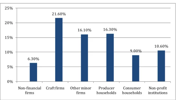
Figure 1: “Credit market share by type of sector” (figures as at 31/12/2008) Source: Federcasse 6.30% 21.60% 16.10% 16.30% 9.00% 10.60% 0% 5% 10% 15% 20% 25% Non-financial firms

Craft firms Other minor firms Producer households Consumer households Non-profit institutions

CBs are rooted in local areas where they reinvest a significant part of their profits. The small geographical ambits, the long-lasting relationships and the in-depth cultural affinity with local firms facilitate financial inclusion as a method of upholding traditional cooperative values. Cooperatives also enhance territorial efficiency by contributing to local development not only in terms of credit granted, but also with the capacity to invest in project selection and in assessing the potential of entrepreneurs and enterprises. The mutualistic nature of CB and the restriction to geographical expansion distinguish their form of enterprise. Cooperative founding principles are based on solidarity and participation of their members mobilised to serve the community. Cooperatives play also an active role at the local level by financing the local economy in this way contributing to the sustainability of local workforces. Due to their proximity to the local economy, CBs are major players when it comes to financing businesses and mainly collect savings which are in turn recycled in the form of loans to the members, to private customers or to small and medium sized enterprises.

Cooperatives differ substantially from stock‑holder companies. CBs accumulate capital by design, as their original purpose was to overcome a shortage of capital for their chosen activities. Further, the opportunities to manage capital in and out are often limited due to statutes and regulations that dictate how capital is managed. Finally, CBs are reliant upon internal capital for strategic investments, whilst the commercial banks

have greater access to raise additional funds, for example through the issuance of stock. Similarly, the demands on capital are less acute. Members of CBs typically take a longer term, risk-adverse view than shareholder-owned banks, with a correspondingly lower expected return. Moreover, financial rewards are not the primary reason for customers, and in some instances employees, to be owners via membership – the provision of good value products and services is assumed to take precedence over profits as a motivating factor.

6 METHOD

The CB risk of failure is assessed using an unbalanced panel38

binary response model. The choice seems the more appropriate because of the nature of bankruptcy data39

. The specific feature of panel data is the possibility of following the same individuals over time, which facilitates the analysis of dynamic responses and the control of unobserved heterogeneity40_{. Moreover, this technique permits to utilise bank-specific and} macroeconomic variables simultaneously and it helps to forecast future financial condition and to focus on risk categories. The probability of future default is obtained as a function of variables drawn from the current period’s financial statements and from macroeconomic information. Furthermore, the precise relationship used to assign bank-failure probabilities are based on the historical relationship observed for bank-failures during a period prior the event of default. The model permits to determine the characteristics that are important to forecast bank failure.

6.1 Model description

Suppose we want to consider the occurrence or non-occurrence of bank failures. It is then mathematically convenient to label one of the groups as success (healthy) and the other as failure (default) and to assign 0 and 1 respectively to indicate whether or not the event has occurred. Then the binary state variable yi equals 1 if bank i failed at ti and it equals 0 otherwise (dummy variable). The choice is especially convenient since it resembles a probability range [0,1]. If we use multiple control variables to explain a binary outcome, the multiple linear regression model is called the linear probability model (LPM) as the response probability is linear in the parameters

β

:

38

Panel data sets with missing years for at least some cross-sectional units (Wooldridge, 2008). 39

Shumway (2001). 40

Arellano (2003). Heterogeneity arises since we are dealing with different individuals (banks). 41

Let us consider a multiple regression model of the following form:

u x x

y=β0 +β1 1+...+βk k +

If we assume that the zero conditional mean assumption holds, that is, E(u|x1,…..,xk)=0, then we get:

k kx x x y E( | )=β0+β1 1+...+β

The key point is that when y is a binary variable taking on the values zero and one, it is always true that P(y=1|x)=E(y|x), leading to Equation 1.

k kx

x y

P( =1|x)=

β

β

β

which says that the probability of success, say p(x)=P(y=1|x), is a linear function of the explanatory variables. In the LPM, βj measures the change in the probability of success when xj changes, holding other factors fixed:

j j x

y

P = = ∆

∆ ( 1|x)

β

The LPM is simple to estimate and use, but it has some limitations. The two most important drawbacks are that the fitted probabilities are not between zero and one and that the partial effect of any explanatory variable is constant42

. These limitations of the LPM can be overcome by using more sophisticated binary response models.

A popular model for discrete dependent-variable is the index function model. The banks’ probability of default is modelled as an unobserved variable y* such that

i i

y* =x_iβ+

ε

( 3 )

where εi is independent of xi (which is a 1 × K vector of control variables with first

element equal to unity for all i) and β is a K × 1 vector of parameters. εi is a random variable and we assume that it has mean zero and has either a standardized logistic with (known) variance π2_{/3 or a standard normal distribution with variance one}43

. The unobserved variable yi* represents the maximum score the subject i can withstand. Instead of observing yi* we observe only a binary variable indicating the change of status (from healthy to problem banks) depending on the sign of yi*:

   > = otherwise if l y if y i i 0 1 * ( 4 )

It is useful to assume that a switch in the status of the banks occurs when a certain “tolerance” l is exceeded. Let us assume l being equal to zero44

. The unconditional expectation of the binary variable y is by definition a probability, such that the vector of

42

Wooldridge (2008). 43

This assumption is an innocent normalization. See Greene (2008) for an extensive discussion of the issue. 44

Again, this assumption is pretty innocent especially as we are considering a regression with a constant term (Greene, 2008).

control variables x is thought to influence the realization of y. The probability of obtaining a failure given a certain set of control variables xi is then given by:

)

(

)

(

1

)

|

(

)

|

0

(

)

|

0

(

)

|

1

(

β

x

β

x

x

β

x

x

β

x

x

x

F

F

P

P

y

P

y

P

=

−

−

=

−

>

=

>

+

=

>

=

=

ε

ε

where F(._{) denotes a cumulative distribution function. The probability of the bank being} healthy is: ) ( 1 ) | 0 (y x F x_iβ P _i = _i = − ( 6 )

By combining expression (5) and (6) it is possible to obtain the conditional distribution of yi given xi: 1 , 0 , )] ( 1 [ )] ( [ ) | ( = − 1− = y F F y f y y i xi xiβ xiβ ( 7 )

These models are generally called index models as they restrict the way the response probabilities depend on the control variables45_{. F is a link function}46 _{taking on values} strictly between zero and one: 0 < F(xiβ) < 1, for all the possible values of the response

variables. This function maps the index into the response probability.

In the logit model F takes on the following form:

) ( )] exp( 1 /[ ) exp( ) (xiβ = xiβ + xiβ =Λ xiβ F ( 8 )

This expression represents the cumulative distribution function (cdf) of the logistic distribution, which is between zero and one for all real numbers z. In the probit model, F is the standard normal cumulative distribution function, which is expressed as an integral:

∫

φ

Where

φ

45

See Wooldridge (2002) for a comprehensive discussion of index models. 46

The link function in generalized linear models specifies a nonlinear transformation of the predicted values so that the distribution of predicted values is one of several special members of the exponential family of distributions (McCullagh, Nelder, 1989). The link function is therefore used to model responses when a dependent variable is assumed to be nonlinearly related to the predictors.

) 2 / exp( ) 2 ( ) ( 1/2 2 β x β x_i =

π

φ

This choice of F again ensures that the estimated response probabilities are strictly between zero and one for all values of the parameters and the covariates.

The functions Λ(xiβ) and Φ(xiβ) are both monotone and increasing functions of xiβ.

These distributions have the familiar bell shape of symmetric distributions. Since the dependent variable was given the value 1 for problem banks and the value 0 for sound banks, positive coefficients will increase the probability of failure, whilst negative ones will be associated with a decrease in the probability of default. Both functions are well-defined probabilities: 0 ) , ( _i

β

β

β

x

β

→

+∞

Longitudinal data permits to analyze the relationship between the event of default and the covariates over time and across individuals. The objective is to estimate CB probability of failure as a function of the predictor variables. For each bank i in the population we have a binary outcome, yit, for each of T time periods. Therefore, yi is a T×1 vector from the cross section, which we assume to be a random draw. As the data set consists of independently sampled observations, we obtain an independently pooled cross section.

In the following analyses and in the estimation of estimated probabilities, two different techniques were considered: pooled cross section regression and unobserved effects models.

6.1.1 Pooled cross section regression

For some vector xit containing any set of observable variables, we specify the distribution of yit given xit. The key assumption in a maximum likelihood framework is that we correctly specify the density of yit given xit. In the panel data setting, partial likelihood is

utilized to get the partial maximum likelihood estimator (PMLE)β∧ 47 :

47

∑∑

where β consist of all parameters appearing in ft (conditional distribution of yit given xit) for any t. In the probit and logit models, a N -consistent estimator of β is obtained by maximizing the partial log-likelihood function:

{

}

∑∑

where F(._{) is the standard normal cdf in the probit model and the logistic cdf in the logit} model. These estimators are consistent and asymptotically normal.

One reason for using independently pooled cross sections is to increase the sample size48 . By pooling data drawn at different points in time, it is possible to obtain more precise estimators and test statistics with more power. In addition, using pooled cross sections raises only minor statistical complications. Furthermore, the usage of general macroeconomic information is justified by the fact that the population may have different distributions in different time periods. Therefore, the intercept is allowed to differ across periods and the general macroeconomic variable serves for this purpose. Nevertheless, pooling is helpful in this regard only if the relationship between the dependent variable and at least some of the independent variables remains constant over time.

6.1.2 Unobserved effects models

An alternative way to use panel data is to take into account unobserved factors affecting the dependent variable. For panel data applications, a popular model for binary outcomes with panel data is the unobserved effects model49

: it it it S u y = + (15) With:

∑

β

β

Where Sit is the score that constitutes an order of the banks according to their riskiness and uit is the unobserved, individual specific heterogeneity. Xit is a vector (p x 1) that can contain a variety of factors, including lagged variables50_{. β is the correspondent (1 x p)} vector of coefficients and it measures the effect on the probability of bank failure of a unit change in the corresponding independent variables. Ci is the (unobserved) heterogeneity.

The estimated response probabilities are given by:

) ( ) | 1 (yit xit it F Sit P = =

λ

where λit gives the probability of default (PD) of bank i at time t. The link function F transforms the score into the PD. This model explicitly takes into consideration unobserved effects that are constant and those that vary over time. Different models can be applied depending on the choice of Ci. The fixed effects regression is equivalent to assume that the effect of omitted variables varies for each individual but is constant over time. This model gives always consistent results but they may not be the most efficient model to run. The between effects control for omitted variables that change over time but are constant between cases. The random effects assumes that some omitted variables may be constant over time but vary between cases, and others may be fixed between cases but vary over time. These models give more efficient estimators.

The choice of F(._{) determines how the coefficients βj are estimated. We have then the} unobserved effects probit and its logit counterpart.

The main assumption of the unobserved effects probit model is:

) ( ) , | 1 ( ) , | 1 (y_it c_i P y_it c_i S_it P = x_i = = x_it =Φ , t=1,...,T (18)

Expression (18) implies strict exogeneity of xit conditional on ci: once ci is conditioned on, only xit appears in the response probability at time t. In addition to (18), it is assumed that the outcomes are independent conditional on (xi, ci):

yi1,...,yiT are independent conditional on (xi, ci) (19)

50

Under assumption (18) and (19) it is possible to derive the conditional density of yit on (xi, ci): ) ; , | ( ) ; , | ,... ( 1 1 xi β t xit i β T t i T c f y c y y f

∏

( β β β . A fixed effects probit analysis is not

possible since it leads to incidental parameters problem. Then, the traditional random effects model adds to (18) and (19) the assumption that ci and xi are independent and

that ci has a normal distribution:

i i x

c | ~ (0, 2)

c

Normal

σ

Since ci has a Normal (0,σ2c) distribution, it is possible to utilize the procedure employed by Butler and Moffitt (1982).The conditional MLE in this context is called the random effects probit estimator51

. An alternative possibility is to implement the approach developed by Zeger, Liang, and Albert (1988) to compute the generalized estimating equations (GEEs). The GEEs have solutions which are consistent and asymptotically Gaussian even when the time dependence is misspecified. The resultant model is called the population-averaged model since the estimated response probabilities can be interpreted as an average value for all individuals with the same covariate structure52

.

The unobserved probit model has logit equivalent. By replacing the logistic cumulative distribution to the standard normal cdf Φ in expression (18) and keeping assumptions (19) and (21), we get the so called random effects logit model. The important advantage over the probit model is that it is possible to obtain N -consistent estimator of β without any assumption about how ci is related to xi53. In this case, using the procedure

implemented by Chamberlain (1984), we can estimate the fixed effects logit estimator. However, as already noticed in some studies54

, this procedure cannot be utilized since only defaulted banks would contribute to the log likelihood and excluding non default banks would generate a biased sample and biased coefficients. Therefore, also for the

51 Wooldridge (2002). 52 Porath (2006). 53 Wooldridge (2002). 54

logit model, we obtain the estimated coefficients by using the GEEs approach and the random effects logit estimator.

6.1.3 Lag structure

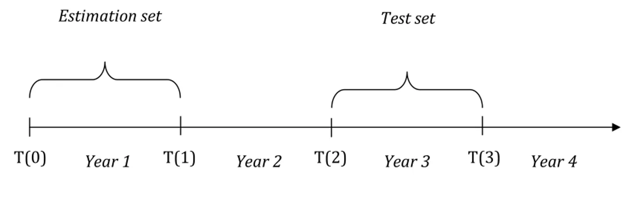
Following the ex-post empirical approach employed in previous bank failure studies55 , the explanatory variables (Xit) are drawn from data for a time period prior to failure. The characteristics of the predetermined groups (healthy and default) are compared considering a time lag permitting to examine the dynamic behaviour. According to the procedure utilized by Gilbert et al. (1999), it is assumed a two year lag (Xit-2) as default events are often the result of the balance sheet audit56

. Thus, the resulting function relates the probability of default in period t to the control variables of period t-2. The econometric model then predicts the likelihood that a bank, currently considered safe and sound, enters default in a period between 12 and 24 months. This procedure permits to have at least a one-year forecast horizon and to include in the analysis a minimum number of failures (34)57

. The model for two years before failure could be used to predict whether a given bank will fail in the future. For instance, we took the financial statements 1998 (Year 1) that, in principle, were available the first day of the next year (Year 2), to predict whether the bank will fail in 2000 (Year 3). As a result, the estimation set had at least a one-year forecast horizon.

Figure 2: Lag structure

55

Among the other studies, Espahbodi (1991), Glennon et al.(2002) and Martin (1977). 56

Porath (2006). 57

By considering a one-year lag, the number of default decreases to 27; in the case of a three-year lag the figure is 25. The decrease in the number of default is given by the unavailability of the financial statements (especially when considering a one-year lag).

Test set Estimation set

A vector of explanatory variables Xit (X1t,X2t,...,Xpt) corresponds to each dependent variable (Yit). The database of the independent variables contains the information (macroeconomic and accounting data) for different individuals (banks) at a given point in time across time (different years).

6.1.4 Test for the contribution of macroeconomic factors

A key purpose of the present research is to analyze the contribution of macroeconomic factors to the estimation of the response probabilities. Thus, the model building process is designed in order to pinpoint the contribution in terms of predictive power and goodness-of-fit of the macroeconomic variables.

In order to test for the contribution of the macroeconomic factors, three different sets of variables and two models (logit and probit) are considered. Different techniques of estimation are employed (pooled regression and the unobserved effects model) in order to estimate the response probabilities under different settings. This procedure leads to more accurate inference since the results are provided under different methodologies.

The first set of covariates includes only bank-level data. Then, after running the model, only variables statistically significant58

are kept in the analysis. In the second set, macroeconomic information is added to the models in the form of macro factors calculated at national level. Again non-significant variables are dropped and only statistically significant variables are considered. This practice permits to evaluate the contribution of the selected general macroeconomic factor to the estimation of the model59

and to determine which variables are significantly related to the response variable. In the third set (full model), local macroeconomic factors are introduced. In the last specification non statistically significant ratios are taken out. Once more, the introduction of the last set allows for inference on the influence of the local environment on the banks’ risk of failure.

58

Significant level at 5%. 59

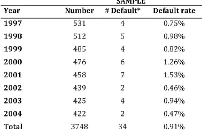
6.2 Sample and data sources

The sample set consists of more than 3,800 observations and includes the financial statements of almost all the Italian Cooperative banks60

. The data span 1997 through 2004. From the original sample, some data has been excluded using the following criteria:

1. the financial statement of the same year of the occurrence of default (3 financial statements);

2. defaulted banks that did not cease to exist after the administrative procedure61 ₍₅₀

financial statements);

3. the financial statement of banks failed during the period of performance one year prior to failure (27 financial statements);

4. banks with incomplete records62 _{(4 financial statements).}

Hence, the resulting total number of observations is 3,748. The sample consists of 604 individuals (banks) and the number of observations per group ranged from 1 to 8. In particular, the participation pattern of the cross-sectional time-series data denotes that for each unit (bank) in the sample, data are not available for all the years.

60

Years 2006, 2007 and 2008 have not been considered since from 1/01/2006 CB have adopted the International Accounting Standards (IAS) in order to prepare the financial statements. The adoption of IAS changes key financial measures and the value relevance of financial statement information, making the data prior and after the introduction of the new standards not homogeneous. Year 2005 has been excluded since during 2007 no events of default were observed.

61

In particular, after the administrative procedure of “amministrazione straordinaria”, a bank could recover and continue its operations.

62

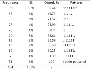
Table 3: “Pattern of cross-sectional time-series data”

Frequency % Cumul. % Pattern

359 59% 59.44 11111111 38 6% 65.73 11…… 35 6% 71.52 111….. 27 4% 75.99 1111…. 26 4% 80.3 1……. 20 3% 83.61 11111… 18 3% 86.59 ...11111 12 2% 88.58 ..111111 10 2% 90.23 111111.. 7 1% 91.39 ....1111 52 9% 100 (other patterns) 604 100% - -

Source: own calculations using data from Federcasse

Looking at the geographical distribution of the CB, almost half of them are located in a single geographical area (North-West 44%) and almost one-fourth in only one region (Trentino Alto-Adige). The total number of CB is decreasing across years due mostly to operation of merger and acquisition.

Table 4: “Number of CB per year and geographical area”

Area 1997 1998 1999 2000 2001 2002 2003 2004 Total Center 87 85 78 87 83 85 81 81 667 North-East 236 228 219 212 206 194 188 186 1669 North-West 78 73 68 64 61 59 58 57 518 South 130 126 120 113 108 101 98 98 894 Total 531 512 485 476 458 439 425 422 3748

Center: Abruzzo, Lazio, Marche, Toscana, Umbria

North-East: Emilia Romagna, Friuli Venezia Giulia, Trentino Alto Adige, Veneto North-West: Liguria, Lombardia, Piemonte, Valle d'Aosta

South: Basilicata, Calabria, Campania, Molise, Puglia, Sardegna, Sicilia

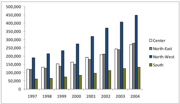
In terms of average total assets and number of branches, the CB in the North-West have a bigger size than CB located in the other areas, especially compared to CB in the South. The average total assets show a positive trend across the areas over the years. CBs in the North-East present the higher growth (138%) whilst CB in the South shows the lower growth (121%) and the lower average number of branches over the period.

Figure 3: Average total assets per year and geographical area(*) 0 50,000 100,000 150,000 200,000 250,000 300,000 350,000 400,000 450,000 500,000 1997 1998 1999 2000 2001 2002 2003 2004 Center North-East North-West South

(*) Data in euro thousands

Figure 4: Average number of branches per year and geographical area

0 2 4 6 8 10 12 14 1997 1998 1999 2000 2001 2002 2003 2004 Center North-East North-West South