Gamma degradation models for earthquake-resistant structures
Iunio Iervolino,1,* Massimiliano Giorgio,2 and Eugenio Chioccarelli.1
1Dipartimento di Ingegneria Strutturale, Università degli Studi di Napoli Federico II, Naples, Italy.
2Dipartimento di Ingegneria Industriale e dell'Informazione, Seconda Università degli Studi di Napoli, Aversa, Italy.
Abstract
Stochastic modeling of deterioration of structures at the scale of the life of the construction is the subject of this study. The categories of degradation phenomena considered are those two typical of structures, that is progressive degradation of structural characteristics and cumulative damage due to point overloads; i.e., earthquakes. The wearing structural parameter is the seismic capacity expressed in terms of kinematic ductility to conventional collapse, as a proxy for a dissipated hysteretic energy damage criterion. The gamma distribution is considered to model damages produced by earthquakes. The exponential distribution is also addressed as a special case. Closed-form approximations, for life-cycle structural assessment, are obtained in terms of absolute failure probability, as well as conditional to different knowledge about the structural damage history. Moreover, gamma stochastic process is considered for continuous deterioration; that is aging. It is shown that if such probabilistic characterizations apply, it is possible to express total degradation (i.e., due to both aging and shocks) in simple forms, susceptible of numerical solution. Finally, the possible transformation of the repeated-shock effect due to earthquakes in an equivalent aging (forward virtual age) is discussed. Examples referring to simple bilinear structural systems illustrate potential applicability and limitations of the approach within the performance-based earthquake engineering framework.
Keywords: stochastic process, life-cycle, performance-based earthquake engineering, cumulative damage, aging.
1. Introduction and formulation
Dependency on history (e.g., number of occurred earthquakes, time elapsed since the last seismic event, or structural repair, etc.) of seismic structural risk may involve all the three elements constituting the performance-based earthquake engineering framework (PBEE) [1], that is, hazard, vulnerability, and loss. History-dependency of seismic hazard is often considered to be related to occurrence of characteristic earthquakes on individual faults, clustering of earthquake sequences, and fault interactions. All of these may be directly linked to the common cause of stress accumulation on the fault, which triggers seismic events. On the other hand, when many independent sources contribute to hazard, in classical probabilistic seismic hazard analysis (PSHA) *Corresponding author: Iunio Iervolino, Dipartimento di Ingegneria Strutturale, Università degli Studi di Napoli Federico II, via
familiar to engineers, it is customary to stochastically model earthquakearrivals via a homogeneous Poisson process (HPP); i.e., a process with independent and stationary increments [2].
Earthquake loss may be time-dependent mainly because of investment costs, which require financial discounting (e.g., [3]), or time-variant occupancy issues. Seismic structural vulnerability, finally, is commonly considered affected by two categories of phenomena that may lead it to vary with time: (1) continuous deterioration of material characteristics, or aging, and (2) cumulating damage because of repeated overloading due to earthquake shocks [4]. Both of them are damage accumulation processes; in the following, aging will be referred to as progressive damage, while damage due to earthquakes will be referred to as shock-based.
Aging, which in some cases may show an effect in increasing seismic structural fragility [5], is often related to an aggressive environment which worsens mechanical features of structural elements, for example: corrosion of reinforcing steel due to chloride attack, or carbonation in concrete; e.g., [6]. To be able to predict the evolution of this kind of wear is especially important in design of maintenance policies (e.g., [7,8]). Often the aging assessment is addressed via predictable
models (e.g., degradation is assumed to evolve deterministically after a random initiation time). In
fact, a stochastic model, which can account for temporal variability of the wear process, can be considered more appropriate [9].
Earthquake shocks potentially cumulate damage on the hit structure during its lifetime, unless partial or total restoration; i.e., within a cycle. In general, mainly because earthquake occurrences can be considered instantaneous with respect to structural life, it is advantageous to model the cumulative seismic damage process separately from the progressive aging. Indeed, to describe earthquakes probabilistically, a marked point process, in which each seismic event is represented by its occurrence time and damage it produces, can be conveniently adopted. With respect to this model, engineering interest is in the compound point process, which accounts for the cumulative damage (i.e., the sum of damage increments) produced by all occurring shocks.
If both deterioration effects may be measured in terms of the same parameter expressing the structural capacity, for example the residual ductility to collapse, or
( )
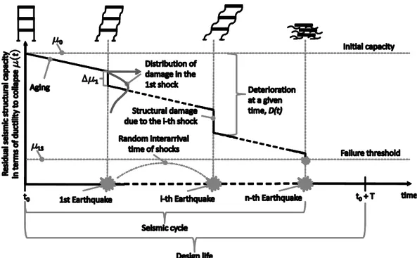
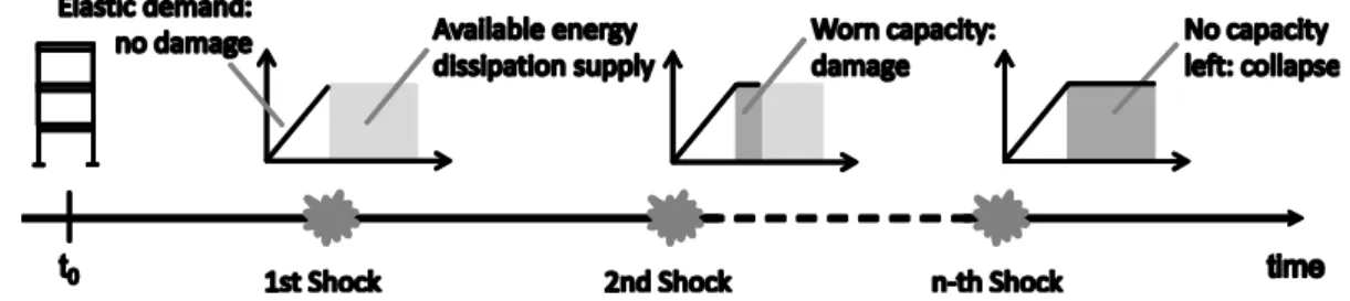
t , then the total wear may be susceptible of the representation as a function of time in Figure 1, where an arbitrary path of the process is depicted, as well as a conventional threshold corresponding to a limit-state of interest.Figure 1. Seismic cycle representation for a structure subjected to aging and repeated earthquake shocks, when degradation affects residual capacity to failure.
Formally, the degradation process is that in Equation (1), where 0 is the initial capacity in the cycle (e.g., the as-new capacity), and D t is the cumulated level of deterioration at the time t.
( )
Note that, with respect to Figure 1, the initial time of the cycle is assumed to be zero, that is t =0 0.
( )
t 0 D t( )
= − (1)
As introduced, D t can be seen as the sum of two effects, one due to continuous deterioration and
( )
one due to accumulation of seismic damage, as in Equation (2), where the first term in the right hand side is the continuous loss of capacity at time t due to aging, C
( )
t , and the second one is the cumulated loss of resistance due to all earthquake events, N t , occurring until time t. Note that( )
( )
C t
( )
( )
( ) 1 N t C i i D t t = = +
(2)Given this formulation, the probability the structure fails within t, P tf
( )
, or the complement to one of the structural reliabilityR t , is the probability that the structure passes a threshold related to a( )
certain limit state, , at any time before t, Equation (3). LS
( )
1( )
( )
( )
( )
0( )
f T LS LS
P t = −R t =F t =P t =P D t − =P D t (3)
In other words, it is the probability that in
( )
0,t the capacity reduces travelling the distance, , between the initial value and the threshold. Note that, by definition, Equation (3) also provides the cumulative probability function (CDF) of structural lifetime, F tT( )
. To model such a risk is the objective of the presented study.The following is structured such that shock-based damage only, that is when continuous deterioration is neglected, is investigated first. The developed compound point process assumes: (1) damage increments, are independent and identically distributed (i.i.d.), (2) the processes regulating earthquake occurrence and seismic damageare mutually independent.
In particular, it is addressed the case in which damage in an individual earthquake is susceptible of gamma representation (including the special case of exponential distribution). For this case, closed- and/or approximate-form solutions for absolute and conditional reliability problems are derived, if earthquake occurrence follows a HPP. The model also considers that not all earthquakes are necessarily damaging, as not all of them are overloads. Indeed, most of the earthquakes occurring in a region where earthquake magnitude follows a Gutenberg-Richter relationship [10] refer to small magnitude events, with negligible (by structural design) consequences, as also discussed later on.
of seismic structural capacity. Then, how to model the total wear when the cumulative earthquake effect and the aging processes may be taken as independent, is approached. Moreover, the special cases, in which total degradation can be described via a single gamma process, are also discussed. The concept of equivalent aging due to earthquake shocks is introduced, which reverting a maintenance concept, is referred to as forward virtual age.
Finally, illustrative applications referring to a simple single degree of freedom (SDOF) elastic-perfectly-plastic (EPP) structure, supposed to be located in a comparatively high-seismicity region in central Italy, are developed to address applications of potential earthquake engineering interest, and to shed some light on suitability of the hypotheses at the basis of these simple age-dependent reliability models.
2. Cumulative earthquake damage
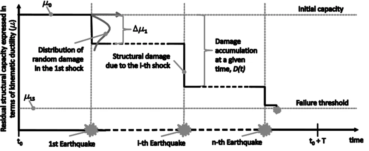
In the case where only shock-based damage is considered (i.e., C
( )
t = 0, t ), then the deterioration process results as sketched in Figure 2 and formulated in Equation (4).Figure 2. Seismic cycle representation for a structure subjected to cumulative earthquake damages only.
( )
0( )
0 ( ) 1 N t i i t D t = = − = −
(4)In the classical case, where the occurrence of seismic events is described by a HPP, N t has a
( )
Poisson distribution with constant rate. Thus, considering the distribution of cumulative earthquake damage as dependent on the number of occurring earthquakes, and their ground motion intensities measures, IM , the failure probability may be computed as in Equation (5), where the integral is of k-th order.
( )
( )
( )
( )
( )
( )
( )
( )
( )
( ) ( ) ( )
1 1 1 1 ! , ! f k k t k k k t i IM k im i P t P D t P D t N t k P N t k t P D t N t k e k t P IM im N t k f im d im e k + = + − = + − = = = = = = = = = = = = =
(5)In the classical HPP-based PSHA, IMs, for example first mode spectral acceleration, Sa, in different earthquakes are i.i.d. RVs, and fIM
( )
im is simply the product of marginal distributions,( )
i IM
f im , which are k in number. Therefore, the critical issue to solve the reliability problem is to get the probability of shock-based damage exceeding the threshold conditional to ground motion
intensities for a given number of earthquakes, that is
( )
1 , k i i P IM im N t k = = =
or, even better,( )
1 k i i P N t k = =
, as per the first line of the equation. The latter may be addressed in a relatively simple manner if three conditions are met, which are listed below.(1) Damage in the i-th earthquake, , always has the same cumulative distribution in i Equation (6), marginal with respect to IM ; i.e., P
i
=P
, . i( )
|
IM( )
im
(2) Damage produced in different events are independent RVs. In other words, according to conditions (1) and (2), earthquake’s structural effects are i.i.d. (This, in particular, implies that a structure, in an earthquake, suffers damage that is independent of its state.)
Condition (3) is that the distribution of sums of damages can be expressed in a simple form. A way to satisfy this condition consists of modeling damage via an RV that enjoys the reproductive property. A well-known example of this kind of variable is the Gaussian one. However, because in earthquakes it should be i 0 i, the deterioration process due to subsequent shocks should also show non-negative increments, rendering the Gaussian representation of damage not perfectly appropriate. Although the lognormal one may appear as a solution (often adopted in the earthquake engineering context), the latter is not reproductive in the addition sense; therefore, it may not be applied if deterioration is seen as the sum of damages.
In the following subsections the gamma RV is considered to derive closed-form solutions for reliability when damage accumulation is due to seismic events only. In fact, the special case of the exponential RV (a gamma distribution with shape parameter equal to one), which literature has already assumed to model damage, is addressed first.
In the application section it will be shown that the gamma distribution may be a suitable option to model earthquake damage, and that the listed conditions apply for an EPP-SDOF if damage accumulation is based on hysteretic energy dissipation. Conversely, they may not be suitable for those systems in which the structural response in one earthquake depends on the previous shock history. The latter is the case of structures with evolutionary or degrading hysteretic behavior and also EPP-SDOF systems when strain-based damage functionals are considered [12]. In these situations, state-dependent approaches (e.g., [13],[14],[15]) may be required to describe, from the reliability point of view, performance degradation.
To model earthquake cumulative damage proceeding in one direction only, the simpler option is the exponential distribution,
( )
DD
f = e− ( is the parameter). The latter was considered as a D possibility in [4], in a useful attempt to provide a framework to stochastically model deterioration of earthquake-resistant structures. In fact, in [4] no closed-form solutions were derived for reliability assessment, albeit, because the sum of i.i.d. exponential RVs is an Erlang-distributed random number. Therefore, the failure probability conditional to k shocks is that given in Equation (7), D
where
( )
1 0 z z e dz + − − =
and U(
,)
1 z y y z e dz + − − =
are the gamma and the upperincomplete gamma functions, respectively. Indeed, the exponential damage assumption yields the
solution of the reliability problem given in Equation (8).
( )
( )
( )
(
( )
)
(
)
( )
(
)
1 1 1 U 0 , ! D D D D D k k D D x D D i D D i D i k D D D i D x P D t N t k P N t k e dx k k e k i − + − = − − = = = = = = = =
(7)( )
( )
(
( )
)
(
)
(
)
(
)
1 1 1 1 0 ! ! ! D D D D D D D D D D k k D D x D t f k D D i k k D D t k i D x t P t P D t e dx e k k t e e i k − + + − − = − + − − = = = = = =
(8)It is to underline that, being continuous and non-negative, the exponential RV is suitable to model only the effect of earthquakes determining loss of capacity, not those events whose intensity is not large enough. In this respect, differently from Equation (5), k in Equation (7) refers to the filtered D HPP of parameter D = P
, counting damaging events only, 0
ND( )
t .The failure probability in Equation (8) can be approximated by the conditional probability in Equation (7), in which ND
( )
t is replaced by expected number of earthquakes until t, Equation (9).1( )
( )
( )
( )
(
(
)
)
(
(
)
)
( )
1 U , D D t D D x D D f D D D D D D x t P t P D t N t E N t e dx t t E N t t − + − = = = =
(9)The latter equation, which is obtained via a rough application of the delta method [16], is expected to be a helpful simplification of the reliability problem. In fact, it is to note that this approximation, to provide results similar to the exact case, requires the neglected terms to be comparatively small with respect to those kept. As shown in the illustrative application later on, this approach, even rough, appears suitable in the context of this study.
2.2. Gamma-distributed damage increments
Although the exponential distribution was already considered to model earthquake damage (e.g., in [4]), one may argue about inherent limited flexibility due to its single parameter. In fact, another option, perhaps more attractive, which depends on two of those and includes the exponential RV as a special case, is the gamma distribution. It is shown in Equation (10), where and D are the D scale and shape parameters, respectively. The use of this continuous non-negative RV, due to its reproductive property, yields handy reliability solutions, similar to those of the exponential case; at the same time, depending on its shape parameter, it can take significantly different shapes. For example, D equal to one stretches the distribution to the exponential, a large value of the shape parameter let the probability density function (PDF) be similar to that of a Gaussian RV, while for
1 To compute Equation (9), the following approximation, yielding the same result of Equation (7) when t is an integer, can be
adopted: ( ) ( ) ( 0.5) 1 U 0 , ! INT i y i y y e i + − − =
.intermediate values of , it is an alternative to the lognormal one to model skewed non-negative D RVs.
( )
D(
D( )
)
D 1 D D f e − − = (10)Because the sum of kD i.i.d. gamma-distributed RVs, with scale and shape parameters and D D
respectively, is still gamma with parameters D and kDD, the probability of cumulative damage exceeding the threshold, conditional to k shocks, is given by Equation (11). Finally, in the gamma D
case, Equation (9) becomes Equation (12), which, again, represents an approximation of P t . f
( )
( )
( )
(
(
)
1)
U(
(
,)
)
D D D k x D D D D D D D D D D D x e k P D t N t k dx k k − − + = = =
(11)( )
( )
( )
( )
(
(
)
)
(
)
(
)
1 U , D D D t D D x f D D D D D D D D D x P t P D t N t E N t e dx t t t − + − = = = =
(12)2.3. Conditional reliability approximations
Formulations above give absolute (i.e., aprioristic) probability that a new structure fails in
( )
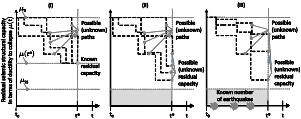
0,t , yet conditional failure probability, which accounts for information possibly available at the epoch of the evaluation, can be obtained. Some of these are given below, and sketched in Figure 3, for different knowledge levels referring to cases in which:(i) the current state of the structure is known at the time of the reliability assessment;
(ii) it is only known that the structure is surviving at the time the evaluation is performed, yet with unknown residual seismic capacity;
(iii) same of (ii) with the additional information about the number of damaging earthquakes the structure was subjected to.
For the sake of generality, all derivations are given for the case damage is a gamma-distributed RV, yet they also apply to the case it is exponential.
Figure 3. Conditional probability cases when: (i) current state is known, (ii) non-collapse (survival) is the only available information; and (iii) when survival and the number of damaging earthquakes are known.
2.3.1. Failure probability when the structural state is known
It may be the case the structure is analyzed at *
t , for example after an earthquake felt in the region where the structure is located, and the current residual capacity is measured,
( )
t* . The failure probability conditional to observed state has the same expression above, just, replacing and t of Equation (9), with *=( )
t* −LS and t t− *, respectively; i.e., Equation (13).(
)
(
(
)
( ))
*(
(
)
)
* * * 1 U * * * * , , − − + − − − = − −
D D D t t D D D D D x f D D D D t t x P t t e dx t t t t t t (13)In fact, the structure has now to undergo a smaller capacity reduction to fail. Equivalent: the same relationship may also be used if the residual capacity * is obtained via a repair at t*.
Also interesting is the case in which one wants to include in the reliability assessment the information that the structure is still surviving at *
t , but with unknown damage condition. It may be computed via Equation (14), plugging in previous results.
( )
( )
( )
( )
(
)
(
)
(
)
* * * * * * * * * 1 | 1 | 1 1 1 1 1 1 1 1 − + − = − = − = − = − = − = − − − −
D D D D f f t x D D D D D DP failure within t t survival in t P survival in t t survival in t
P survival in t t survival in t R t P t P survival in t R t P t x e dx t x
(
)
(
)
(
)
(
)
(
)
* U * 1 U * * , 1 1 , 1 − + − − = − −
D D D D D D D t D D D x D D D D t t t e dx t t (14)2.3.3. Failure probability when survival and the number of damaging earthquakes are known
Finally, the probability of failure given survival at *
t and the number, ND
( )
t* =kD (larger thanzero), of damaging earthquakes until *
t , yields Equation (15), where the approximation is analogous to those above.
( )
( )
( )
( )(
)
(
)
* * * * * * * * 1 * * 1 * * * * 1 0 , 1 1 1 1 1 1 D D D D D D D D k N t t i i D D k D D i i k k i D D D D i kP failure within t t survival in t N t k
P P T t T t N t k P T t N t k P P N t t k P N t t k + − = = + + = = = = − = = − = − = = − − − = − = = −
(
)
( )(
)
(
)
(
)
(
)
(
)
(
)
(
)
* 1 * 1 U * * 1 U 1 , 1 1 1 1 , 1 1 D D D D D D D D D k i i k t t D D D D D x D D D D D D D D D D k D D D x D D D D D D P k t t x e dx k t t k t t k x e dx k k = + − − + − − + − = − + − − − + − + − − = − − −
(15)Note that in the case ND
( )
t =* 0, Equation (12) applies, in which t is replaced by*
t t− ; i.e., in
absence of damaging shocks, the structure is as new at t*.
3. Gamma process for continuous wear modeling
This section refers to the modeling of aging. The key difference with respect to the shock-based damage discussed so far, is that its probabilistic representation is a continuous process, resulting in progressive wear. An attractive option is the gamma process that, if applicable, implies that degradation has independent and stationary gamma-distributed increments, yielding Equation (16) for the PDF of wear accumulated in
( )
0,t . It may prove suitable to model continuously accumulating degradation, such as wear, fatigue, corrosion, crack growth, creep, swell; i.e., typical aging-related phenomena in structures [17]; however, the properties of the increment imply that degradation accumulation in any time interval only depends on how wide such interval is, independent of current state and age of the structure.( )
( )
(
(
)
)
1 A A C s t A A t A f e s t − − = (16)In Equation (16) the deteriorating structural parameter is still ductility to collapse, thus it is assumed the phenomenon affects seismic capacity. Therefore, if degradation is due to aging only, the failure probability is given by Equation (17).
( )
( )
( )
(
(
)
)
1 U(
(
,)
)
− + − = = = =
A A s t A A x A A f C A A x s t P t P D t P t e dx s t s t (17)Note that the model of Equation (16) also implies the mean and the variance of the degradation process vary linearly being equal to: E
C( )
t =(
sA
A)
t and Var
C( )
t =(
sA
A2)
t . Despite this assumption, which helps to keep the illustration simple and is also considered in thestructural context (e.g., [9],[17],[18]), it is to recall that if the shape parameter is defined as a non-linear function of time, the gamma process allows to model degradation trends different from that linear (i.e., non-stationary increments).
4. Degradation due to shock-based damage and aging
In the case the point and continuous degradation processes are independent and modeled as in sections 2.2 and 3, then the failure probability is that given in Equation (18), which follows from Equation (9) and Equation (17). It may be easily solved numerically; however, it is to mention that analytical-form for the convolution of an arbitrary number of independent gamma random variables, with different parameters, may also be derived; see [19].
( )
( )
( )
( ) ( )( )
( )(
)
( )
(
)
(
)
(
(
)
)
1 1 0 1 1 0 0 1 1 1 N t C i i D D A D A N t f C i i D t t s t y D D x A A y D D A P t P D t P t F F y f y dy x y e e dx dy t s t = = − − − − − = = + = = − = − − = −
(18)The use of Equation (18) has an important implication. It assumes that the progressive damage accumulation process continues in the same fashion independently of earthquake damage; i.e., occurrence of a seismic damage does not alter future evolution of progressive deterioration. Thus, for example, from the practical point of view, if aging is due to chloride penetration and steel corrosion, it is assumed that evolution of this process is not significantly affected by crack openings due to earthquakes. Specular: damage resulting from an earthquake is independent of both age and amount of deterioration the structure is found when the earthquake occurs.
Due to the properties of the gamma distribution, also invoked in section 2.2, it follows that in the case continuous aging and seismic damage share the same scale parameter, , probability of failure, conditional to the number of shocks, kD, is that of Equation (19).
( )
( )
(
(
)
)
1 U(
(
,)
)
| A D D s t k A D D x D D A D D A D D x s t k P D t N t k e dx s t k s t k + − + − + = = =
+ + (19)The assumption yielding this equation may be restrictive and has to be verified case-by-case. Obviously, when it applies, Equation (19) gives evident computational advantages. On the other hand, also in the case the hypothesis is not verified, it may be used to quickly obtain a preliminary estimate of the failure probability, to be refined further if needed.
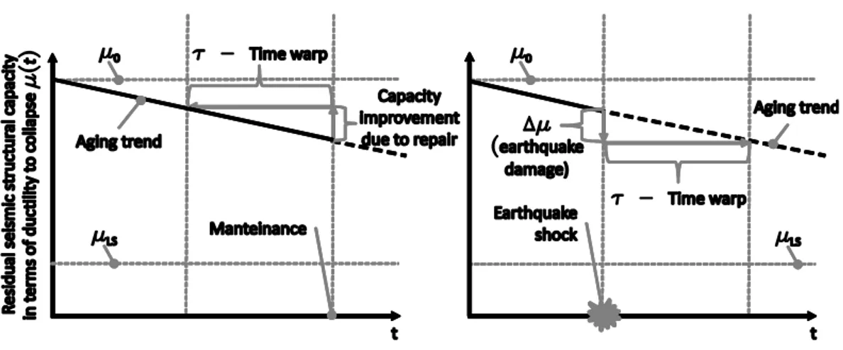
It is also worth noting, as a side result, that Equation (19) is susceptible of an appealing interpretation, in terms of the virtual age concept, originally developed to account for the effect of maintenance in the reliability assessment [20]. According to virtual age, repair is seen as rejuvenation, such that, from the reliability assessment point of view, the repaired system is equivalent to the original one, but with an age reduced by the number of years cancelled by repair (Figure 4, left).
Figure 4. Backward virtual age from repairable systems’ maintenance theory (left); forward virtual age, that is, continuous deterioration equivalent to earthquake damage (right).
In fact, in the case under study, the effect of the shock may be seen as equivalent to aging. Indeed, defining the time warp = D sA, Equation (19) may be rewritten as Equation (20), which shows
that failure probability of a structure of age t and subject to kD earthquakes, may be computed as
that of a structure with age t+kD , and no shocks. This model may be referred to as forward
virtual age (as opposite to that backward of [20]).
( )
( )
(
)
(
)
(
)
( )(
)
(
(
)
)
1 U | | 0 , A D D D D D D s t k A D x A D A D P D t N t k P D t k N t k s t k x e dx s t k s t k + − + − = = + + = = + = = + +
(20)4.2. Life-cycle and conditional reliability approximations
Equation (19) allows the derivation of handy approximations of reliability considering both degradation phenomena; the failure probability may be approximated as in Equation (21), with the use of the same approximation as in Equation (9). In fact, if the equivalent shape parameter,
A D D
s=s + , is introduced, the term at the second line of the Equation (21) coincides with that of Equation (17).
( )
(
)
( )( )
(
)
(
)
(
)
( )
(
( )
)
1 1 1 1 U 1 , + − + − + + − − − + − = = + + = =
D A D D A D A s t E N t s t s x x f A D D D A D A s t x x x P t e dx e dx s t E N t s t s x s t e dx s t s t (21)Conditional probabilities, given the same pieces of information discussed in section 2.3, can be also retrieved for this model. In particular, if the current residual seismic capacity,
( )
*t
, is measured
at a certain time *
t , the failure probability is that of Equation (22).
(
)
(
(
)
( ))
( )(
)
(
( )
)
(
)
* * * * 1 U * * * * , , LS s t t LS x f t s t t t x P t t e dx t t s t t s t t − − + − − − − − = − −
(22)Recalling Equation (21) and Equation (14), if the information is only that the structure is still surviving at *
t , the failure probability is approximated by Equation (23). If the number of damaging earthquakes is also known, Equation (24), applies.
(
)
( )
(
)
( )
(
)
( )
(
)
( )
* 1 U * * * 1 U * * , 1 1 | 1 1 , 1 1 − + − − + − − − − = − − −
s t x s t x x s t e dx s t s tP failure within t t survival in t
s t x e dx s t s t (23)
( )
(
)
( )(
)
(
)
(
)
(
)
* * * * * 1 * 1 * * U , 1 1 1 , 1 1 A D D D D A D D D D s t k t t x A D D D D s t k x A D D A D D D D AP failuire within t t survival in t N t k
x e dx s t k t t x e dx s t k s t k t t s t + + − − + − + − + − = = − + + − − = − + + + − − = −
(
)
(
)
(
)
* * U * , 1 D D D D A D D A D D k t t s t k s t k + + − + − + (24)5. Illustrative application
In this section structural modeling is addressed with reference to a simple EPP-SDOF system with unloading/reloading stiffness, which is the same as the initial one. The reason to choose this model is threefold: (i) it is at the basis of earthquake engineering and the results developed for it are expected to be of significant generality; (ii) earthquake-resistant structures, especially those reflecting modern codes, may be often rendered equivalent to this kind of system; (iii) it shows stable hysteretic cycles that repeat themselves despite of the sequence of excitation it undergoes. This latter property is especially important with respect to the age-dependent reliability models discussed herein, which are based on independent and identically distributed damage increments. In
the following, earthquake-based cumulative damage is addressed first, subsequently, continuous deterioration, and finally the sum of the two.
5.1. Structural response and ductility-based collapse criterion
The elastic period of the EPP-SDOF is equal to 0.5 s; weight is 100 kN and the yielding force
( )
Fyis equal to 19.6 kN, which corresponds to a strength reduction factor equal to 2.5 given a 0.49 g spectral acceleration.
Chosen engineering demand parameter (EDP) is the kinematic ductility,
; i.e., the maximum displacement, when the yielding displacement is the unit. In fact, such an EDP is chosen as the simplest proxy for the dissipated hysteretic energy during one earthquake event. Note that this implies, as in all energy-based damage measures, structural damage in all seismic events with intensity larger than that required to yield the structure; see also [21] for a discussion.The collapse is assumed to occur when kinematic ductility, conservatively accumulated independently on the sign of maximum displacement, reaches some capacity value.
If the considered limit state (LS) is collapse prevention (CP) derived from [22], which assumes conventional collapse of concrete structures at a maximum drift ratio equal to 0.04, the system has an (initial) ductility capacity 0 =3.3, and each damaging shock drains some of this ductility supply (Figure 5).
Figure 5. Accumulation of damage in shock sequence with respect to kinematic ductility for EPP-SDOF system.
Once structural system and collapse criterion are defined, it is possible to address the i.i.d. hypothesis of damage increments. Due to its force-displacement relationship, the considered SDOF
this means the maximum displacement reached in the i-th earthquake of a sequence (required to compute the ductility assumed to be related to the dissipated energy) is just the same as if the damaging event hit the new structure, plus the residual displacement from the preceding shaking. In other words, according to the assumed damage criterion, variation of drained capacity in the i-th earthquake is independent both of the age and the state the shock finds the structure in. Thus, different earthquakes produce i.i.d. effects, independent of the structural conditions.
5.2. Evaluating the distribution of damage increments
The marginal CDF of the damage increment in a shock, , may be computed via Equation (6), where fIM
( )
im is derived from the HPP hazard curve for the site where the structure is supposed tobe located. The probabilistic seismic demand term, f|IM
(
|IM =im)
, may be computed viaincremental dynamic analysis (IDA) assuming the spectral acceleration at the elastic period of the
SDOF, as an IM.2 IDA is developed in terms of structural ductility normalized by 0, in a way that the demand is equal to 1 when the CP-LS is attained. Thus, may be defined as in Equation (25), where
before and
after refer to residual capacity before and after the generic earthquake shock.0 before after − = (25)
Figure 6 (left) shows IDAs3 output for the considered EPP system; in the same figure, recalling the normalization of ductility demand, collapse limit corresponding to 1, is also reported. Figure 6 (right) shows f|IM
(
|IM =im)
for some ground motion intensities, under the assumption they are lognormal RVs (a well-established hypothesis in PBEE context).2 Due to the mentioned repetitive features of the EPP response, it is also easy to show that a single set of IDAs is required to estimate
the distribution of damage increments given IM (see [23] for details).
3 To develop IDAs thirty records were selected via REXEL [24], with moment magnitude between 5 and 7, epicentral distances
Figure 6. Ductility demand from IDA analyses (left) and some distributions of structural damage conditional to ground motion intensity (right).
Marginalization of the distribution of damage increments by fIM
( )
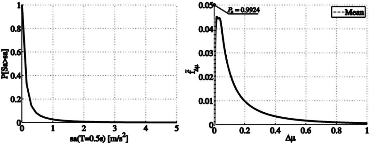
im , as per Equation (6), is site-specific. Considered site is (arbitrarily) Sulmona (13.96 Lon.; 42.05 Lat.), close to L’Aquila in central Italy. PSHA for the site was carried out by software specifically developed and described in [26], to which the reader should refer for details. fIM( )
im for the spectral ordinate corresponding to the SDOF’s elastic period, is reported in Figure 7 (left). Note that, it is not exactly the hazard curve for the site, while it is the distribution of ground motion intensity given the occurrence of anearthquake. In fact, this is required to obtain the marginal distribution of capacity reduction in one
shock, and it was obtained from the hazard curve divided by the annual rate of occurrence of events in Sulmona, which is equal to 1.95 (between magnitude 4.3 and 7.3).
Figure 7. Complementary CDF of ground motion intensity given earthquake occurrence at the site of interest (left); marginal distribution of for the structure at the site of interest (right).
In Figure 7 (right), the result of the marginalization in Equation (6) is reported. To comment on the plot it has to be recalled that, given the structure, not all earthquakes are strong enough to yield the structure, and = 0 for such shocks. In particular, is larger than zero only for spectral accelerations larger than about 1.96 m/s2, which is, in fact, the yielding acceleration of the
considered EPP. Thus, damage increment is not a continuous RV and its CDF has the expression in Equation (26).
( )
( )
0 0 0 0 0 f x P F P P dx
= + = =
(26)In other words, the distribution of
is defined by means of a probability density for 0, and a probability mass for = 0 . In fact, P0= =P
0 accounts for the probability thatearthquakes are not strong enough to damage the structure. Also P
has an interesting 1
meaning; it is the marginal (i.e., with respect to earthquakes magnitude and location) probability that the new structure fails in just one event. In this application P =
0 and P
are equal 1
to 0.9924 and 0.0006, respectively. This means that only 0.76% of earthquakes is expected to be damaging, while 0.06% is expected to be catastrophic; i.e., directly causing collapse.The expected value of
, E
= 0.0026, is also reported, yet barely visible, in Figure 7 (right). It means that, for the considered structure at the considered site, a generic earthquake produces a capacity reduction of about 0.26%, on average with respect to both damaging and undamaging events. Thus, referring to the seismic hazard of Sulmona, given that average number of earthquakes in one year is equal to 1.95, the considered SDOF is expected to undergo an average capacity reduction equal to 0.0026 1.95 =0.0051 or 0.5% per year. Therefore, according to the considered criterion, the structure fails after about 200 years on average.5.3. Absolute and conditional reliability for the cumulative earthquake damage case
The gamma distribution is adopted to model the PDF of shock effect in the case of damage larger than zero,
f
( )
=f
( )
/ 1 P(
− 0)
; see section 2.2. Scale, D, and shape, D, parameters of the model are set equal to 0.5539 and 0.1916, respectively.The criterion to calibrate the gamma distribution was to set its mean and variance equal to the conditional mean and variance of damage (in the case it is larger than zero) computed by means of the structural analysis described in the previous section. Therefore, the scale and shape parameters were obtained solving the equations D D =E
0
=0.3459 and
2
0 0.6245
= =
D D Var
; where 0.3459 and 0.6245 are the mean and variance of the curve
in Figure 7 (right), when its area is normalized to one.
Failure probabilities are computed in the following illustrative cases: (1) failure probability within 50 yr, Equation (12); (2) failure probability within 50 yr given that after the first 25 yr a reduction of 30% of the as-new capacity has been measured, Equation (13); (3) failure probability within 50 yr given that no collapse was recorded in the first 25 yr, Equation (14); and (4) failure probability within 50 yr given that one damaging earthquake hit the structure without causing collapse in the first 25 yr, Equation (15). Results are given in Equation (27), where it also recalled that the expected number of damaging earthquakes is computed filtering the all earthquakes HPP.
( )
( )( )
( )( )
( )( )
(
)
25 0.3 25 1 25 1, 1 0 (1) 50 0.076 (2) 50 0.0524 (3) 50 0.0407 (4) 50 0.047 1, 2, 3 1 0.0076 1.95 D f f D f D f D k D D P P P P k t P t t = = = = − = (27)At this point, it is appropriate to check tolerability of the gamma-assumption for the damage increments. Moreover, it is the occasion also to verify the implications of using the approximation,
based on the delta method, in Equation (12). To this aim, in Figure 8 (left) the CDF of the lifetime of the structure, F tT
( )
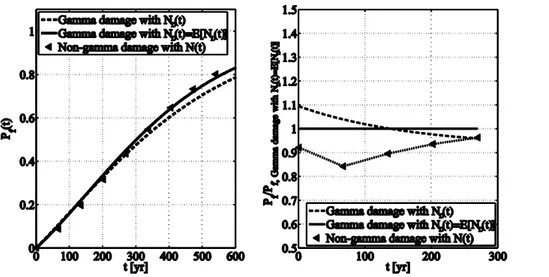
, according to the model in Equation (12), is reported.Figure 8. Structural lifetime distribution in the case of earthquake damage according to the approximated model of Equation (12) and removing the approximation of the gamma distribution for the damage increments and the
expect number of shocks in lieu of any number of earthquakes.
In the same figure, P t is also computed: (i) under the assumption damage increments are f
( )
gamma distributed and explicitly considering the probability associated to any number of shocks as in Equation (5); and (ii) adopting for the empirical distribution obtained from structural simulation, and explicitly considering the probability associated to any number of shocks. The figure shows that, at least up to three hundred years, where failure probability is 0.6 (hardly tolerable for a civil construction), the gamma assumption, even in case of the delta-method-based approximation, gives results in agreement with those of the empirical model (on the safe side). This is quantitatively shown by the ratios in Figure 8 (right), which are computed taking as a reference
( )
f
P t from the gamma-based model.
5.4. Total degradation and virtual age
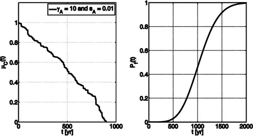
This section starts considering the case of a structure subject (only) to continuous deterioration of seismic capacity that can be described via a gamma process with mean and variance function
3
10
A A
s
=t − t and(
sA
A2)
t 104 t−
= , respectively. The corresponding process, and the CDF of
lifetime, are reported in Figure 9; it emerges that it was assumed continuous deterioration has a mild effect (in accordance to literature; e.g., [18]), and the structure has a median life of about 1000 yr, while Pf is close to one after about 2000 yr, if this is the sole source of degradation. This arbitrary
choice was to simulate aging mildly affecting seismic capacity if compared to shock-based damage.
Figure 9. Realization of continuous deterioration process (left); corresponding lifetime CDF (right).
In the case effects of earthquake and aging are independent, the failure probability due to both can be computed numerically solving Equation (18), in which
D, D
and
A,sA
are equal to
0.5539, 0.1916 and
10,0.01 , respectively. Resulting lifetime distribution is reported of Figure
10, along with analogous results for the two individual processes.Assume now the same scale parameter, for example that of cumulative earthquake damage, can be attributed to both degradation processes. For example, imposing that A =D, the shape parameter
of continuous deterioration process may be reshaped such that the same linear trend is preserved, that is sA=D EC
( )
t ; however, this implies to force the variance of the process to be t(
2)
A D
s t. In this case, if 3 3 10 0.5539 10
A D
s = − = − , the same mean of aging in Figure 9 is kept,
yet the variance results to be VarC
( )
t =0.0018t. This allows to apply Equation (21) with
= D,s= +sA D D
parameters, Equation (28).
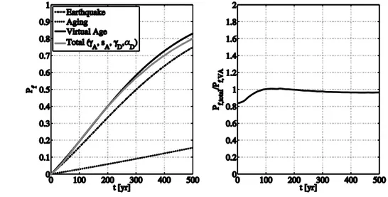
3 3 1 | 0 0.5539 0.5539 10 1 0.01482 0.3459 0.0034 0.5539 10 A D A s s E s − − = + = = + = (28)The resulting lifetime CDF, compared with individual and total degradations, is given in Figure 11 (left), where also suitability of the approximation is depicted (Figure 11, right). It may be deduced that, in this particular case, the approximation provided by the simple model, appears acceptable.
Along the same line, it is also possible to get results analogous to Equation (27) using Equation (21), Equation (22), Equation (23), and Equation (24). Results are given in Equation (29).
( )
( )( )
( )( )
( )( )
25 0.3 25 1 25 1, 1 (1) 50 0.0920 (2) 50 0.0629 (3) 50 0.0499 (4) 50 0.0572 D f f D f D f D k P P P P = = (29)It is interesting to note that, according to the parameters of the application,
(
3)
0.1916 0.5539 10 346
D sA yr
= = − = , meaning that a generic damaging earthquake is
illustrates how the forward virtual age concept, if applicable, is attractive: it provides, at a glance, vulnerability of a structure subject to the considered sources of deterioration.
Figure 11. Lifetime CDFs (left); failure probability ratio of superimposed degradations and virtual age, or VA (right).
6. Conclusions
Life-cycle reliability analysis of deteriorating structures was discussed. The addressed approach potentially accounts for both progressive aging and damage accumulation due to earthquake shocks. The structural performance measure considered is the ductility capacity to collapse as a simplistic proxy for an energy-based damage criterion. This has the advantage to enable treating aging and earthquake damage effects altogether.
First, models for reliability analysis of structures cumulating seismic damage were discussed in the case of exponential and gamma distributions. Closed- and/or approximate-form reliability solutions were formulated; these also enable accounting for information possibly available at the epoch of the evaluation. Second, the gamma-process, especially suitable to represent continuous wear due to its non-negative, independent, and stationary increments characteristics, was adopted to model structural progressive damage accumulation. Then, reliability of structures, subject to both degradation phenomena, was formulated in the case of independent gamma-based processes.
The suitability of the discussed reliability model in the performance-based earthquake engineering context was also illustrated via a simple application, which refers to a bilinear SDOF system located in a relatively high seismicity site in central Italy. Conventional collapse prevention limit-state was considered and the gamma distribution’s parameters were calibrated based on structural analysis, with reference to dissipated hysteretic energy damage indices. The results of the models were also discussed with respect to invoked assumptions and approximations.
Results support the conclusion that gamma-process-based stochastic modeling of degrading structures, may be useful in the performance-based earthquake engineering context.
Acknowledgements
The study was developed in the framework of AMRA – Analisi e Monitoraggio dei Rischi Ambientali scarl (http://www.amracenter.com). The results refer to the Strategies and tools for Real-Time Earthquake Risk Reduction (REAKT; http://www.reaktproject.eu) and to the New Multi-Hazard and Multi-Risk Assessment Methods for Europe (MATRIX; http://matrix.gpi.kit.edu/), projects. REAKT and MATRIX are funded by the European Community via the
Seventh Framework Program for Research (FP7), with contracts no. 282862 and no. 265138, respectively. Authors
want finally to thank Ms. Racquel K. Hagen, of Stanford University, for proofreading the paper.
References
1. Cornell, C.A., Krawinkler, H. (2000) Progress and challenges in seismic performance assessment. Peer Center
Newletter, 3(2).
2. McGuire, R.K. (2004) Seismic Hazard and Risk Analysis, Earthquake Engineering Research Institute, MNO-10, Oakland, California, 178 pp.
3. Yeo, G.L., Cornell, C.A. (2009) Building life-cycle cost analysis due to mainshock and aftershock occurrences.
Struct. Saf., 31(5), 396–408.
4. Sanchez-Silva, M., Klutke, G.-A., Rosowsky, D.V. (2011) Life-cycle performance of structures subject to multiple deterioration mechanisms. Struct. Saf., 33(3), 206–217.
5. Rao, A., Lepech, M., Kiremidjian, A., Sun, X.Y. (2010) Time varying risk modeling of deteriorating bridge infrastructure for sustainable infrastructure Design. In Frangopol, D.M., Sause, R, and Kusko, C.S., (eds.), Bridge
Maintenance, Safety, Management, and Life-Cycle Optimization. Proc. of the Fifth International Conference on Bridge Maintenance, Safety and Management (IABMAS), Philadelphia, PA.
6. Stewart, M.G., Wang, X., Nguyen, M.N. (2011) Climate change impact and risks of concrete infrastructure deterioration. Eng. Struct., 33(4), 326–1337.
7. Frangopol, D.M., Kallen, M.-J., van Noortwijk, J.M. (2004) Probabilistic models for life-cycle performance of deteriorating structures: review and future directions. Prog. Struct. Eng. Mat., 6(4), 197–212.
8. Ellingwood, B., Mori, Y. (1997) Reliability-based service life assessment of concrete structures in nuclear power plants: optimum inspection and repair. Nuc. Eng. Des., 175(3), 247-258.
9. Pandey, M.D., van Noortwijk, J.M. (2004) Gamma process model for time-dependent structural reliability analysis. In Watanabe, E., Frangopol, D.M., Utsonomiya, T., (eds.), Bridge maintenance, safety, management and
cost. Proc. of the Second international conference on bridge maintenance, safety and management (IABMAS),
Kyoto, Japan.
10. Gutenberg, R., Richter, C.F. (1944) Frequency of earthquakes in California, B. Seism. Soc. Am., 34(4), 185-188. 11. Çinlar, E. (1980) On a generalization of gamma processes. J. Appl. Prob., 17(2), 467-480.
12. Cosenza, E., Manfredi, G. (2000) Damage indices and damage measueres, Prog. Struct. Eng. Mat., 2(1), 50-59. 13. Luco, N., Bazzurro, P., Cornell, C.A. (2004) Dynamic versus static computation of the residual capacity of a
mainshock-damaged building to withstand an aftershock. Proc. of the 13th World Conference on Earthquake
Engineering. Vancouver, Canada. Paper No. 2405.
14. Giorgio, M., Guida, M., Pulcini, G. (2011) An age- and state-dependent Markov model for degradation processes,
IIE T., 43(9), 621-632.
15. Giorgio, M., Guida, M., Pulcini, G. (2010) A state-dependent wear model with an application to marine engine cylinder liners. Technometrics, 52(2), 172-187.
16. Oehlert, G.W. (1992) A note on the delta method.The American Statistician, 46(1), 27-29.
17. Van Noortwijk, J.M., van der Weide, J.A.M., Kallen, M.J., Pandey, M.D. (2007) Gamma processes and peaks-over-threshold distributions for time-dependent reliability. Reliab. Eng. Syst. Saf., 92(12), 1651-1658.
18. Vamvatsikos, D., Dolsek, M. (2011) Equivalent constant rates for performance-based assessment of aging structures. Struct. Saf., 33(1), 8-18.
19. Johnson, N.L., Kotz, S. (1970) Continuous Univariate Distributions, 1 and 2, Wiley, New York.
20. Kijima, M. (1989) Some results for repairable systems with general repair. J. Appl. Prob., 26(1), 89-102.
21. Iervolino, I., Giorgio, M., Chioccarelli, E., (2013) Closed-form aftershock reliability of damage-cumulating elastic-perfectly-plastic systems. Earthq. Engn. Struct. Dyn. (in press)
22. Federal Emergency Management Agency (2000) Prestandard and commentary for the seismic rehabilitation of
buildings. Report FEMA 356. Washington DC.
23. Chioccarelli, E., Iervolino, I. (2012) In Impact of repeated events with various intensities on the fragility functions
for a given building typology at local scale. D4.1 of the MATRIX project (URL http://matrix.gpi.kit.edu/).
24. Iervolino, I., Galasso, C., Cosenza, E. (2010) REXEL: computer aided record selection for code-based seismic structural analysis. B. Earthq. Eng., 8(2), 339–362.
25. CEN, European Committee for Standardization. (2003) Eurocode 8: Design provisions for earthquake resistance
of structures, Part 1.1: general rules, seismic actions and rules for buildings, Pren1998-1.
26. Iervolino, I., Chioccarelli, E., Convertito, V. (2011) Engineering design earthquakes from multimodal hazard disaggregation. Soil. Dyn. Earthq. Eng., 31(9), 1212–1231.