Thermoelectric efficiency of three-terminal quantum thermal machines

(1)

PAPER • OPEN ACCESS

Thermoelectric efficiency of three-terminal

quantum thermal machines

To cite this article: Francesco Mazza et al 2014 New J. Phys. 16 085001

View the article online for updates and enhancements.

-thermal machines

Francesco Mazza1, Riccardo Bosisio2, Giuliano Benenti3,4, Vittorio Giovannetti1, Rosario Fazio1and Fabio Taddei1

1_{NEST, Scuola Normale Superiore, and Istituto Nanoscienze-CNR, I-56126 Pisa, Italy} 2

Service de Physique de l’ État Condensé (CNRS URA 2464), IRAMIS/SPEC, CEA Saclay, 91191 Gif-sur-Yvette, France

3

CNISM and Center for Nonlinear and Complex Systems, Universitá degli Studi dell’ Insubria, via Valleggio 11, 22100 Como, Italy

4_{Istituto Nazionale di Fisica Nucleare, Sezione di Milano, via Celoria 16, 20133 Milano, Italy}

E-mail:francesco.mazza@sns.it

Received 3 April 2014, revised 23 May 2014 Accepted for publication 27 May 2014 Published 7 August 2014

New Journal of Physics 16 (2014) 085001

doi:10.1088/1367-2630/16/8/085001

Abstract

The efficiency of a thermal engine working in the linear response regime in a multi-terminal configuration is discussed. For the generic three-terminal case, we provide a general definition of local and non-local transport coefficients: elec-trical and thermal conductances, and thermoelectric powers. Within the Onsager formalism, we derive analytical expressions for the efficiency at maximum power, which can be written in terms of generalized figures of merit. Further-more, using two examples, we investigate numerically how a third terminal could improve the performance of a quantum system, and under which condi-tions non-local thermoelectric effects can be observed.

Keywords: thermoelectric and thermomagnetic effects, nonequilibrium and irreversible thermodynamics, electronic transport in mesoscopic systems

1. Introduction

Thermoelectricity has recently received enormous attention due to the constant demand for new and powerful ways of energy conversion. Increasing the efﬁciency of thermoelectric materials,

Content from this work may be used under the terms of theCreative Commons Attribution 3.0 licence. Any further distribution of this work must maintain attribution to the author(s) and the title of the work, journal citation and DOI.

(3)

in the whole range spanning from macro- to nano-scales, is one of the main challenges of great importance for several different technological applications [1–6]. Progress in understanding thermoelectricity at the nanoscale will have important applications for ultra-sensitive all-electric heat and energy transport detectors, energy transduction, heat rectiﬁers and refrigerators, just to mention a few examples. The search for optimization of nano-scale heat engines and refrigerators has hence stimulated a large body of activity, recently reviewed by Benenti et al [7].

While most of the investigations have been carried out in two-terminal setups, thermoelectric transport in multi-terminal devices has just begun to be investigated [8–22] since these more complex designs may offer additional advantages. An interesting perspective, for instance, is the possibility to exploit a third terminal to ‘decouple’ the energy and charge ﬂows and improve thermoelectric efﬁciency [9–12, 16–19]. Furthermore, fundamental

questions concerning thermodynamic bounds on the efﬁciency of these setups has been

investigated [13–15, 20, 21], also accounting for the effects of a magnetic ﬁeld breaking the time-reversal symmetry [23]. In most of the cases studied so far, however, all but two-terminals

were considered as mere probes; i.e. no net ﬂow of energy and charge through them was

allowed. In other works a purely bosonic reservoir has been used, only exchanging energy (and not charge) current with the system [9–12].

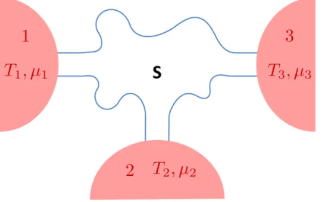
A genuine multi-terminal device will however offer enhanced flexibility and therefore it might be useful to improve thermoelectric efficiency. A full characterization of these systems is still lacking and motivates us to tackle this problem. Here we focus on the simplest instance of three reservoirs, which can exchange both charge and energy current with the system. A sketch of the thermal machine is shown in figure 1, where three-terminals are kept at different temperatures and chemical potentials connected through a scattering region. Our aim is to provide a general treatment of the linear response thermoelectric transport for this case, and for this purpose we will discuss local and non-local transport coefficients. Note that non-local transport coefficients are naturally requested in a multi-terminal setup, since they connect

Figure 1. Three-terminal thermal machine. A scattering region is connected to three different fermionic reservoirs, each of these is able to exchange heat and particles with the system. Reservoir 3 is taken as the reference for measuring temperature and energy: T3≡ T; μ3 = . The reservoirs 1 and 2 have small variations in temperature andμ chemical potential: T( ,i μi) = (T+ ΔTi,μ+ Δμi), i∈ (1, 2). With S we denote a generic coherent cattering region.

(4)

temperature or voltage biases introduced between two-terminals to heat and charge transport among the remaining terminals. We will then show that the third terminal could be exploited to improve thermoelectric performance with respect to the two-terminal case. We will focus our investigations on the efficiency at maximum power [24–33], i.e. of a heat engine operating under conditions where the output power is maximized. Such quantity, central in thefield of finite-time thermodynamics [34], is of great fundamental and practical relevance to understand which systems offer the best trade-off between thermoelectric power and efficiency.

The paper is organized as follows. In section 2 we briefly review the linear response, Onsager formalism for a generic three-terminal setup. We will discuss the maximum output power and trace a derivation of all the local and non-local transport coefficients. In section3we extend the concept of Carnot bound at the maximum efficiency to the three-terminal setup and we derive analytical formulas of the efficiency at maximum power in various cases, depending on the flow of the heat currents. These expressions are written in terms of generalized dimensionlessfigures of merit. Note that the expressions derived in sections2and3 are based on the properties of the Onsager matrix and on the positivity of the entropy production. Therefore they hold for non-interacting as well as interacting systems. This framework will then be applied in section4to specific examples of non-interacting systems in order to illustrate the salient physical picture. Namely, we will consider a single quantum dot and two dots in series coupled to the three-terminals. Finally section5 is devoted to the conclusions.

2. Linear response for 3-terminal systems

The system depicted in figure 1 is characterized by three energy and three particle currents (J_iU₌_1,2,3and J_iN₌_1,2,3, respectively)flowing from the corresponding reservoirs, which have to fulfill the constraints: J J 0 (energy conservation) , 0 (particle conservation) , (1) i i U i i N 1 3 1 3

∑

= = = =

(positive values being associated withﬂows from the reservoir to the system). In what follows we will assume the reservoir 3 as a reference and the system to be operating in the linear response regime, i.e. set

(

T3, μ3

)

≡ ( , )T μ and write

(

Tj, μj

) (

= T + ΔTj, μ + Δμj

)

with

k T

/ 1

j B

Δμ

| | ≪ and |ΔT T_j|/ ≪ 1 for j=1,2, and k_B is the Boltzmann constant. Under these

assumptions the relation between currents and biases can then be expressed through the Onsager matrix L of elements L_ij via the identity:

J J J J L L L L L L L L L L L L L L L L X X X X , (2) N Q N Q T T 1 1 2 2 11 12 13 14 21 22 23 24 31 32 33 34 41 42 43 44 1 1 2 2 = μ μ ⎛ ⎝ ⎜ ⎜ ⎜ ⎜⎜ ⎞ ⎠ ⎟ ⎟ ⎟ ⎟⎟ ⎛ ⎝ ⎜ ⎜ ⎜ ⎜ ⎞ ⎠ ⎟ ⎟ ⎟ ⎟ ⎛ ⎝ ⎜ ⎜ ⎜ ⎜ ⎜ ⎞ ⎠ ⎟ ⎟ ⎟ ⎟ ⎟

(5)

where X_1,2μ = Δμ_1,2/T and X_1,2T = ΔT_1,2/T2 are the generalized forces, and where

J_1,2Q = J_1,2U − μ_{1,2 1,2}JN are the heat currents of the system, the corresponding currents to reservoir 3 being determined from J_1,2N and J_1,2Q via the conservation laws of equation (1). In our analysis we take L to be symmetric (i.e. L_ij = L_ji) by enforcing time reversal symmetry in the problem. We also remind that, due to the positivity of the entropy production rate, such a matrix has to be semi-positive deﬁnite (i.e. L ⩾ ) and that it can be used to describe a two-terminal model0 connecting (say) reservoir 1 to reservoir 3 by setting L_j₃ = L_j₄ = L₃_j = L₄_j = 0 for all j. 2.1. Transport coefficients

For a two-terminal model the elements of the Onsager matrix L can be related to four quantities which gauge the transport properties of the system under certain constraints. Specifically these are the electrical conductance G and the Peltier coefficient Π (evaluated under the assumption that both reservoirs have the same temperature), and the thermal conductance K and the thermopower (or Seebeck coefficient) S (evaluated when no net charge current is flowing through the leads). When generalized to the multi-terminal model these quantities yield to the introduction of non-local coefficients, which describe how transport in a reservoir is influenced by a bias set between two other reservoirs.

2.1.1. Thermopower. For a two-terminal conﬁguration the thermopower relates the voltageΔV

that develops between the reservoirs to their temperature differenceΔT under the assumption that no net charge current is ﬂowing in the system, i.e. S

( )

V_T

JN 0

= − Δ_Δ

= . A generalization of this

quantity to the multi-terminal scenario can be obtained by introducing the matrix of elements

S e T , (3) ij i j J k T k j 0 , 0 kN k Δμ Δ = − Δ = ∀ = ∀ ≠ ⎛ ⎝ ⎜ ⎞ ⎠ ⎟

with local (i = j) and non-local (i ≠ j) coefficients, e being the electron charge. In this definition, which does not require the control of the heat currents, we have imposed that the particle currents in all the leads are zero (the voltages are measured at open circuits) and that all but one temperature differences are zero (of course this last condition is not required in a two-terminal model). It is worth observing that equation (3) differs from other definitions proposed in the literature. For example in [35] a generalization of the two-terminal thermopower to a three-terminal system, was proposed by setting to zero one voltage instead of the corresponding particle current. While operationally well defined, this choice does not allow one to easily recover the thermopower of the two-terminal case (in our approach instead this is rather natural, see below). Finally in the probe approach presented in [8, 13–15, 20, 21] it was possible to study a multi-terminal device by using an effective two-terminal system only, because the heat and particle currents of the probe terminals are set to vanish by definition. Therefore, within this approach, there are no chances of having non-local transport coefficients.

In the three-terminal scenario we can use equation (2) to rewrite the elements of the matrix (3). In particular introducing the quantities

(6)

we get (see appendix A for details) S eT L L S eT L L 1 , 1 , (5) 11 13;32 (2) 13;31 (2) 22 14;31 (2) 13;31 (2) = = S eT L L S eT L L 1 , 1 , (6) 12 13;34 (2) 13;31 (2) 21 13;21 (2) 13;31 (2) = =

which yields, correctly, S₁₁ _eT1 L_L12 11

= as the only non-zero element, by taking the two-terminal

limits detailed at the end of the previous section.

2.1.2. Electrical conductance. In a two-terminal conﬁguration the electric conductance describes how the electric current depends upon the bias voltage between the two-terminals under isothermal conditions, i.e.G

( )

eJ

V T 0 N = Δ Δ =

. The generalization to many-terminal systems is provided by the following matrix:

G_ij e Ji . (7) N j T k k j 2 0 , 0 k k Δμ = Δ Δμ = ∀ = ∀ ≠ ⎛ ⎝ ⎜⎜ ⎞_⎠⎟⎟

Using the three-terminal Onsager matrix (2) we ﬁnd

G G G G e T L L L L , (8) 11 12 21 22 2 11 13 13 33 = ⎛ ⎝ ⎜ ⎞_⎠⎟ ⎛_⎝⎜ ⎞ ⎠ ⎟

which, in the two-terminal limit where reservoir 2 is disconnected from the rest, gives

G₁₁= e_T2L₁₁as the only non-zero element.

2.1.3. Thermal conductance. The thermal conductance for a two-terminal is the coefﬁcient which describes how the heat current depends upon the temperature imbalance ΔT under the assumption that no net charge current is ﬂying through the system, i.e. K

( )

J_T

J 0 Q N = _Δ = . In the multi-terminal scenario this generalizes to

K J T , (9) ij i Q j J k T k j 0 , 0 k N k Δ = Δ = ∀ = ∀ ≠ ⎛ ⎝ ⎜ ⎞ ⎠ ⎟

where one imposes the same constraints as those used for the thermopower matrix (3), i.e. no currents and ΔT_k = 0 for all terminals but the jth. For a three-terminal case, using equation (4) this gives K T L L L L L L L 1 , (10) 11 2 13 12;32 (2) 12 13;32 (2) 11 23;23 (2) 13;31 (2) = − − K T L L L L L L L 1 , (11) 22 2 14 13;43 (2) 13 14;43 (2) 11 34;34 (2) 13;31 (2) = − −

(7)

and K K T L L L L L L L 1 . (12) 12 21 2 24 13;31 (2) 14 13;23 (2) 34 13;12 (2) 13;31 (2) = = + +

Once more, in the two-terminal limit where the reservoir 2 is disconnected from the rest, the only non-zero element is K

T L L 11 1 2 12;12 (2) 11 = .

2.1.4. Peltier coefficient. In a two-terminal conﬁguration the Peltier coefﬁcient relates the heat current to the charge current under isothermal conditions, i.e.

( )

J

eJ T 0 Q N Π = Δ = . For multi-terminal systems this generalizes to the matrix

J eJ , (13) ij i Q j N T k k j 0 , 0 k k Π = Δ Δμ = ∀ = ∀ ≠ ⎛ ⎝ ⎜⎜ ⎞ ⎠ ⎟⎟

which can be shown to be related to the thermopower matrix (3), through the Onsager

reciprocity equations, i.e. Π_ij( )B = TS_ji(−B) (B being the magnetic ﬁeld on the system), [36, 37] from which, using equations (5) and (6), one can easily derive for the three-terminal case the dependence upon the Onsager matrix L.

3. Efﬁciency for 3-terminal systems

In order to characterize the properties of a multi-terminal system as a heat engine we shall now analyze its efficiency. Generalizing the definition for the efficiency of a two-terminal machine [7, 36], we define the steady state heat to work conversion efficiency η, for a three-termianl machine, as the powerW˙ generated by the machine (which equals to the sum of all the heat currents exchanged between the system and the reservoirs), divided by the sum of the heat currents absorbed by the system, i.e.

W J J J J J , (14) i i Q i i Q i i Q i i i N i i Q 1 3 1 2 η= ˙ Δμ ∑ = ∑ ∑ = −∑ ∑ = = + + +

where the symbol∑_i

+ in the denominator indicates that the sum is restricted to positive heat

currents only, and where in the last expression we used equation (1) to express J₃Q in terms of the other two independent currents5.

The deﬁnition (14) applies only to the case in whichW˙ is positive. Since the signs of the heat currentsJ_iQ are not known a priori (they actually depend on the details of the system), the

5

Note that equation (14) can be easily generalized to M terminals, after appropriate change of the numerator. By setting for instance

(

TM,μM

)

=( , )T μ ,ΔTi=Ti−T, and Δμi=μi−μ(i= 1 ,...,M− ), the output power reads1

as follows: W J J . (C.5) i M i Q i M i i N 1 1 1

∑

Δμ ˙ = = − = = −

(8)

expression of the efficiency depends on which heat currents are positive. For the three-terminal system depicted in figure 1 we set for simplicity T₃ < T₂ < T₁ and focus on those situations where J₃Q is negative (positive values of J₃Q being associated with regimes where the machine effectively works as a refrigerator which extracts heat from the coldest reservoir of the system). Under these conditions the efficiency is equal to

W JQ JQ , (15) 12 1 2 η = ˙ +

when both J₁Q and J₂Q are positive, or

W J , (16) i i Q η = ˙

when for i = 1 or 2 only J_iQ is positive.

3.1. Carnot efficiency

The Carnot efficiency represents an upper bound for the efficiency and is obtained for an infinite-time (Carnot) cycle. For a two-terminal thermal machine the Carnot efficiency is obtained by simply imposing the condition of zero entropy production, namely

S˙ = ∑_{i i}JQ/T_i = . If the two reservoirs are kept at temperatures T0 ₁ and T₃ (with T₃ < T₁), from the deﬁnition of the efﬁciency, equation (14), one gets the two-terminal Carnot

efﬁciency 1 T T/

C II

3 1

η = − . The Carnot efﬁciency for a three-terminal thermal machine is

obtained analogously by imposing the condition of zero entropy production, when a reservoir at an intermediate temperature T₂ is added. If J₁Q only is positive as in equation (16), one obtains

(

)

(

)

T T J J J J 1 1 1 , (17) C Q Q C II Q Q ,1 3 1 2 1 32 2 1 32 η = − + − ζ = η + − ζ

whereζ ≡_ij T T_i/ _j. Note that equation (17) is the sum of the two-terminal Carnot efﬁciency η_CII

and a term whose sign is determined by

(

1− ζ₃₂

)

. Since J₁Q > , J0 ₂Q < 0 andζ < , it follows₃₂ 1 thatη_C,1is always reduced with respect to its two-terminal counterpartη . Analogously if only_CII

J₂Q is positive, one obtains

(

)

(

)

T T J J 1 1 , (18) C C II Q Q ,2 3 1 1 2 13 12 η = η − ⎡ − ζ − − ζ ⎣ ⎢ ⎤ ⎦ ⎥ which again can be shown to be reduced with respect to

C II

η , since J₁Q < , J0 ₂Q> ,0 ζ > , and₁₂ 1 1

13

ζ > . We notice that this is a hybrid conﬁguration (not a heat engine, neither a refrigerator):

the hottest reservoir absorbs heat, while the intermediate-temperature reservoir releases heat. However, the heat to work conversion efﬁciency is legitimately deﬁned since the generation of power (W˙ > ) can occur in this situation. Finally, if both0 J₁Q and J₂Q are positive as in equation (15) one obtains

(9)

T T T T 1 1 1 1 1 1 . (19) C J J C II J J ,12 3 1 12 3 1 12 Q Q Q Q 1 2 1 2 η = − + ζ − η ζ + = − − + ⎛ ⎝ ⎜ ⎜ ⎞ ⎠ ⎟ ⎟

Since T₃ < T₂ < T₁, the term that multiplies T T₃/ ₁is positive so thatη_C,12is reduced with respect to the two-terminal case.

It is worth noticing that, in contrast to the two-terminal case, the Carnot efﬁciency cannot be written in terms of the temperatures only, but it depends on the details of the system. Moreover, note that the Carnot efﬁciency is unchanged with respect of the two-terminal case if

T₂ = T₃ in (17) or ifT₂ = T₁ in (19). Indeed, in this situation the quantitiesζ_ij are equal to one, making the extra terms in equations (17) or (19) vanish.

The above results for the Carnot efﬁciency could be generalized to many-terminal systems. In particular, we conjecture that, given a system that works between T₁and T₃ (with T₃ < T₁) and adding an arbitrary number of terminals at intermediate temperatures will in general lead to Carnot bounds smaller than

C II

η . On the other hand, adding terminals at higher (or colder)

temperatures than T₁ and T₃ will makeη_C increase.

Notice that within the linear response and via equation (2) we can express the Carnot efﬁciencies (17)–(19) in terms of the generalized forces X_1,2μ.

3.2. Efficiency at maximum power

The efficiency at maximum power is the value of the efficiency evaluated at the values of chemical potentials that maximize the output powerW˙ of the engine. In the two-terminal case the efficiency at maximum power can be expressed as [28]

(

W

)

ZT ZT 2 2 , (20) II C II max η ˙ = η + where ZT GS T K 2

= is a dimensionlessﬁgure of merit which depends upon the transfer coefﬁcient of the system. The positivity of the entropy production imposes that such quantity should be non-negative (i.e. ZT⩾ ), therefore0 ηII

(

W˙_max

)

is bounded to reach its maximum value /2

C II

η

only in the asymptotic limit of ZT → ∞ (Curzon–Ahlborn limit [24–27] within linear response [28]).

For the three-terminal conﬁguration the output power is a function of the four generalized forces

(

X₁μ, X₁T, X₂μ, X₂T

)

introduced in equation (2), i.e.

(

)

W˙ = −T J X₁N ₁μ + J X₂N ₂μ . (21)

In the linear regime this is a quadratic function which can be maximized with respect toX₁μand

X₂μwhile keeping X₁T and X₂T constant (the existence of a maximum being guaranteed by the the positivity of the entropy production). The resulting expression is

(

)

W T X X M X X 4 , , (22) T T T T max 4 1 2 1 2 ˙ ₌ ⎛ ⎝ ⎜⎜ ⎞ ⎠ ⎟⎟

(10)

where M c a

a b

= ⎡⎣ ⎤⎦ is a positive semi-deﬁnite matrix, see appendixB, whose elements depend on the Onsager coefﬁcients via the identities

a G S S G S S G S S G S S b G S G S S G S c G S G S S G S , 2 , 2 . (23) 12 12 21 12 11 22 22 21 22 11 11 12 11 12 2 12 12 22 22 22 2 11 11 2 12 21 11 22 21 2 = + + + = + + = + +

Indicating withα > β ⩾ 0 the eigenvalues of M we can then further simplify equation (22) by writing it as

(

)

W˙_max= α cos2θ+ β sin2θ X T2 4 4 , (24)

whereX =

( )

X₁T 2 +

( )

X₂T 2 is the geometric average of system temperatures, while the angleθ identiﬁes the rotation in the X₁T, X₂T plane which deﬁnes the eigenvectors of M. We call the parameter

P = α cos2θ + β sin2θ (25)

three-terminal power factor. It relates the maximum power to the temperature difference: by construction it fulﬁlls the inequalityβ ⩽ P ⩽ α, the maximum being achieved forθ =0(i.e. by ensuring that

(

X₁T, X₂T

)

coincides with the eigenvector of M associated with its largest eigenvalue α). Note that in the two-terminal limit we have β → ,0 α → G S_{11 11}2, cos2θ → , so1 that the usual two-terminal power factor G S_{11 11}2 is recovered.

Exploiting equation (24) we can now write the efﬁciency at maximum power for the three cases detailed in equations (15) and (16). Speciﬁcally we have

(

)

(

)

(

)

W T T Z T T Z T Z T y Z T Z T 1 2 2 2 2 , (26) c b a a c 1 max 1 11 2 1 11 11 1 11 11 η Δ Δ δ δ ˙ ₌ + + ˜ + + + − −

(

)

(

)

(

)

W T T Z T T Z T Z T y Z T Z T 1 2 2 2 2 , (27) b c a a b 2 max 2 22 1 22 22 22 22 η Δ Δ δ δ ˙ ₌ + + + + + and

(

)

(

)

(

)

(

)

(

W

)

T T Z T T Z T Z T y Z T Z T y Z T Z T 1 2 2 2 1 2 1 , (28) c a b a b a c 12 max 1 12 2 12 1 12 1 1 12 12 1 12 12 η Δ Δ δ δ ˙ ₌ + + + + + + + ˜ + + − − − −

where we have deﬁned the parametersδ = X₁T/X₂T = ΔT₁/ΔT₂, y= K₁₂/K₂₂and y˜ = K₁₂/K₁₁and introduced the following generalized ZT coefﬁcients:

Z T aT K Z T bT K Z T cT K , , . (29) ij a ij ij b ij ij c ij = = =

The efﬁciencies (26), (27) and (28) can also be expressed in terms of the corresponding Carnot efﬁciencies given in equations (17), (18) and (19), obtaining the following equations which mimic equation (20) of the two-terminal case:

(11)

(

W

)

Z T Z T Z T y y y Z T Z T Z T T C T 2 2 2 4 2 2 2 , (30) C b a c b a c C 1 max ,1 11 11 2 11 2 11 11 2 11 ,1 11 1 11 η η δ δ δ δ δ δ η ˙ ₌ + + ˜ + ˜ + + + + = +  

(

W

)

Z T Z T Z T y y y Z T Z T Z T T C T 2 2 2 4 2 2 2 , (31) C b a c b a c C 2 max ,2 22 22 2 22 2 22 22 2 22 ,2 22 2 22 η η δ δ δ δ δ δ η ˙ ₌ + + ˜ + + + + + = +  

(

)

(

)

(

)

W Z T Z T Z T o T y y Z T Z T Z T o T T C T 2 2 2 4 2 2 2 , (32) C b a c i b a c i C 12 max ,12 12 12 2 12 1 2 1 12 12 2 12 ,12 12 12 12 η η δ δ Δ δ δ δ δ Δ η ˙ ₌ + + + + + ˜ + + + + ≃ + − −  

where we have introduced the constants

C₁= 2y y˜ + 4δy˜ + 2 ,δ2 (33)

C₂ = 2δ2y y˜ + 4δy + 2, (34)

C₁₂ = ˜y−1 + δ2y−1 + 2 ,δ (35)

and the combinations of ﬁgures of merit

(

)

T Z 2 Z Z T . (36) ij ij b ij a ij c 2 δ δ = + + 

Notice also that in writing equation (32) we retained only the leading order neglecting contributions of order ΔT_i or higher.

The above expressions can be used to provide a generalization of the Curzon–Ahlborn limit efficiency for a multi-terminal quantum thermal device. Indeed using the Cholesky decompositions on the Onsager matrix, we can prove that the constants C₁, C₂ defined in equations (33), (34) are positive, see appendix B for details. This fact together with the positivity of the quantities_iiT, that we have checked numerically, implies that the efficiencies

(

W

)

i max

η ˙ are always upper bounded by half of the associated Carnot efﬁciencies, i.e.

(

W

)

2 , (37)

i max C i,

η ˙ ⩽ η

the inequality being saturated when the generalized ZT coefﬁcients (29) diverge. An analogous conclusion can be reached also for (32), yielding

(

W

)

2 . (38)

C

12 max ,12

η ˙ ⩽ η

In this caseC₁₂ is no longer guaranteed to be positive due to the presence of K₁₂. Still the inequality (38) can be derived by observing that the quantitiesC₁₂ and₁₂T entering in the rhs of equation (32) have always the same sign.

4. Examples

In this section we shall apply the theoretical framework developed so far to two specific non-interacting systems attached to three terminals. Namely, we will discuss the case of a single dot and the case of two coupled dots, in the absence of electron–electron interaction (which cannot be dealt within the Landauer–Büttiker formalism). Our aim is to show that one can easily find situations where the efficiency and output power are enhanced with respect to the two-terminal

(12)

case. Furthermore, through the example of the single dot, weﬁnd the conditions that guarantee the non-local thermopowers to vanish.

The coherentflow of particles and heat through a non-interacting conductor can be described by means of the Landauer–Büttiker formalism. Under the assumption that all dissipative and phase-breaking processes take place in the reservoirs, the electric and thermal currents are expressed in terms of the scattering properties of the system [38–40]. For instance, in a generic multi-terminal configuration the currents flowing into the system from the i-th reservoir are:

J h dE E f E f E 1 ( ) ( ) ( ) , (39) i N j i ij i j

∫

∑

= − ≠ −∞ ∞ ⎡ ⎣ ⎢ ⎢ ⎤ ⎦ ⎥ ⎥ 

(

)

J h dE E E f E f E 1 ( ) ( ) ( ) , (40) i Q j i i ij i j

∫

∑

μ = − − ≠ −∞ ∞ ⎡ ⎣ ⎢ ⎢ ⎤ ⎦ ⎥ ⎥ 

where the sum over j is intended over all but the ith reservoir, h is the Planckʼs constant,_ij( )E is the transmission probability for a particle with energy E to transit from the reservoir j to reservoir i, and whereﬁnally f E_i ( )

{

exp

(

E _i

)

/k T_B _i 1

}

1

μ

= − +

−

⎡⎣ ⎤⎦ is the Fermi distribution of the particles

injected from reservoir i (notice also that we are considering currents of spinless particles). In what follows we will use the above expressions in the linear response regime where|Δμ|/k T_B ≪1and

T T/ 1

Δ

| | ≪ , and compute the associated Onsager coefﬁcients (2), see appendix C. 4.1. Single dot

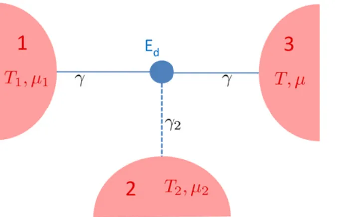
In this section we study numerically a simple model consisting of a quantum dot with a single energy level E_d, coupled to three fermionic reservoirs, labeled 1, 2, and 3, see ﬁgure 2. For simplicity, the coupling strength to electrodes 1 and 3 are taken equal toγ, while the coupling

Figure 2.Sketch of the single dot model used in the numerical simulations: a quantum dot with a single energy level E_d is connected to three fermionic reservoirs 1, 2, and 3. The chemical potential and temperature of the reservoir 3 are assumed as the reference valuesμ and T. The constants γ andγ₂ represent the coupling between the system and the various reservoirs (see C.1 for details). A zero value of γ₂ corresponds to disconnecting the reservoir 2 from the system: in this regime the model describes a two-terminal device where reservoirs 1 and 3 are connected through the single dot.

(13)

strength to electrode 2 is denoted byγ₂. In particular we want to investigate how the efﬁciencies, output powers and transport coefﬁcients evolve when the system is driven from a two-terminal

to a three-terminal conﬁguration, that is by varying the ratio /

2

γ γ. The two-terminal conﬁguration corresponds to γ =₂ 0 and the third terminal is gradually switched on by increasingγ γ. As detailed in appendix₂/ C, the transmission amplitudes between each pair of terminals can be used to evaluate the Onsager coefﬁcients L_ij—the resulting expression being

provided in equations (C.4). Once the matrix L_ij is known, all the currents flowing through the system, efficiencies, output powers and transport coefficients can be calculated within the framework developed in the previous sections.

4.1.1. Efficiencies and maximum power. In ﬁgure 3 we show how the Carnot efﬁciency η_C

depends on the temperature differencesΔT₁andΔT₂, when the chemical potentials are chosen to guarantee maximum output power, i.e.,ﬁxing the generalized forces X_1,2μ in order to maximize

W˙. As we can see, η_C increases linearly along any ‘radial’ direction deﬁned by a relation

T₂ k T₁

Δ = Δ , where k is a constant. In particular, the dashed lines corresponding to k = 0.5, k = 2, and k= − separate the different regimes discussed in section1 3.1: for− <1 k < 0.5the system absorbs heat only from reservoir 1 (if ΔT₁> ) or from 2 and 3 (if0 ΔT₁< ); for0

k

0.5 < < 2.0the system absorbs heat from reservoirs from 1 and 2 (if ΔT₁> ) or from 3 only0

Figure 3. Carnot efficiency η (density plot) of the three-terminal system depicted in_C figure2, as a function of the gradients of temperature in reservoirs 1 and 2 (the chemical potentials μ and₁ μ being chosen to guarantee maximum output power W₂ ˙ ). The coupling with the reservoirs have been set to have a symmetric configuration with respect to 1 and 2 (i.e.γ₂= ). Note thatγ η increases linearly along any radial direction_C defined by a relation TΔ ₂= k TΔ ₁, where k is a constant. In particular, the dashed lines corresponding to k = 0.5, k = 2 and k = − separate different regimes discussed in1 section 3.1. The numbers in each region identify the reservoirs from which the heat is absorbed. Parameter values:γ = 0.2k T_B , E_d −μ= 2.0k T_B .

(14)

(if ΔT₁< );0 ﬁnally, for k> 2 and k< − 1the system absorbs heat only from reservoir 2 (if

T₂ 0

Δ > ) or from 1 and 3 (if ΔT₂ < ). In the case where only one heat0 flux is absorbed the Carnot efficiency is given by equation (17) or (18), while it is given by equation (19) if two heat fluxes are absorbed.

In ﬁgures 4 and 5, we show how the efﬁciency equation (14), the output power

equation (21), the efﬁciency at maximum output power equations (26)–(28) and the maximum output power equation (22), vary when the system is driven from a two-terminal to a three-terminal conﬁguration, i. e. by varying the ratio /

2

γ γ. We set opposite signs for

1

Δμ and

2 Δμ , so

Figure 4.Left panel: efﬁciency η, normalized over the associated Carnot limit computed as in section 3.1, as a function of the coupling to the reservoir 2. Note that as γ γ₂/ is switched on, the efﬁciency increases until it reaches a maximum aroundγ₂∼ 0.3γ, and then it decreases. Right panel: output power W˙ extracted from the system, as a function of the coupling to the reservoir 2. Parameters: γ = 0.1k T_B , Ed −μ= 2.0k TB ,

k T 5 10 _B 1 2 4 Δμ = −Δμ = − × − _, _T ₁₀ _T 1 3 Δ = − , and ΔT₂ = .0

Figure 5. Left panel: efﬁciency at maximum power η

(

W˙max

)

, normalized over the Carnot limit, as a function of the coupling to the reservoir 2. Right panel: maximum output power W˙_max extracted from the system, as a function of the coupling to the reservoir 2. Parameters:γ = 0.1k T_B , E_d− μ=2.0k T_B , ΔT₁= 10−3T, and ΔT₂= .0

(15)

that the system absorbs heat only from the hottest reservoir 1, andΔT₂ = , in such a way that0 the Carnot efﬁciency

C

η coincides with that of a two-terminal conﬁguration, namely

T T

1 /

C 1

η = − . Interestingly, we proved that increasing the coupling

2

γ to the reservoir 2 may lead to an improvement of the performance of the system. In particular, as shown inﬁgure6, the efﬁciency and the output power can be enhanced at the same time at small couplings γ₂, exhibiting a maximum around γ₂ ∼ 0.3γ andγ₂ ∼ 0.6γ, respectively.

In ﬁgure 5 we show results for the same quantities but at the maximum output power [η

(

W˙_max

)

andW˙_max]. In this case, whileW˙_max still increases withγ₂, the corresponding efﬁciency decreases approximately linearly.

In ﬁgures6 and7we show the same quantities as in ﬁgures4 and5, but as a function of the couplingγ for two values ofγ₂ (γ =₂ 0and 0.5

2

γ = γ). Fromfigure6we can see that at small γ the coupling to a third terminal can enhance both the efficiency (for γ ≲ 0.8k T_B ) and the power (forγ ≲ k T_B ). Infigure7we note that, both for the two- and the three-terminal systems, the efficiency at maximum power tends to /η η =_C 0.5in the limitγ → , while the output power0 vanishes. For the two-terminal the result is well known, since a delta-shaped transmission function leads to the divergence of the figure of merit ZT [41–43]. Correspondingly, the efficiency at maximum power saturates the Curzon–Ahlborn bound /η η =_C 0.5. The same two-terminal energy-filtering argument explains the three-terminal result. Indeed, we found numerically that for γ →0 the chemical potentials optimizing the output power are such that

2 3

μ = μ. Since also the temperatures are chosen so that T₂ = T₃, we can conclude that terminals 2 and 3 can be seen as a single terminal.

4.1.2. Thermopowers. In this section we show analytically that the non-local thermopowers are always zero in this model, while the local ones are equal. We consider a general situation,

Figure 6.Left panel: efﬁciency η, normalized over the Carnot limit, as a function of the coupling energy γ. Right panel: Output power W˙ extracted from the system, as a function of the coupling energy γ. In both cases, the full red curves correspond to a three-terminal conﬁguration with γ₂= 0.5γ, while the dashed blue curves refer to the two-terminal case (γ = ). Parameters: E₂ 0 _d −μ= 2.0k T_B , 1 2 10 k TB

4

Δμ = −Δμ = − − ,

T₁ 10 3T

(16)

with three different coupling parameters:γ₁= ,γ γ₂ = cγ andγ₃= d γ, with c ≠ d. Under these assumptions, the transmissions are given at the end of appendix C. Substituting these expressions in equations (5) and (6), weﬁnd:

S S eT L L S S 1 , 0 . (41) 11 22 1 0 21 12 = = = =

This result is a direct consequence of the factorization of the energy dependence of the transmission probabilities, which are all proportional to the same function , as shown in equation (C.3). Such factorization allows us to rewrite the Onsagerʼs coefﬁcients as in equation (C.4) and derive equation (41). The fact that the non-local thermopowers, for example

S₁₂, are zero can be understood as follows. Consider ﬁrst the case in which T₁= T₂ = T₃ and terminal 2 behaves as a voltage probe. If so, from the condition J₂N = L X₃₁ ₁μ+ L X₃₃ ₂μ = 0 we derive Δμ₂ = −

(

L₃₁/L₃₃

)

Δμ₁. Due to the factorization of the energy dependence in the

transmissions we obtain

(

/

(

)

2 1 1 3 1

Δμ = γ γ + γ Δμ. Hence,

1

Δμ does not depend on the coupling

2

γ. If in particular we consider

2

γ = , because of the symmetry of the system under exchange ofγ

the terminal 1 and 3 we have μ₁ = μ₃. We can therefore conclude that, independently of the coupling γ₂, the probe voltage condition for terminal 2 implies Δμ = . It can be shown that₁ 0 such a result remains valid even when ΔT₁= 0 but ΔT₂ ≠ , as requested in the calculation of0 the thermopowerS₁₂. As a result,S₁₂ = 0. The same argument can be repeated for the current J₁N with the terminal 1 acting as a voltage probe, leading to S₂₁= .0

Figure 7. Left panel: efﬁciency at maximum power η

(

W˙_max

)

, normalized over the Carnot limit, as a function of the coupling energy γ. Right panel: Maximum output power W˙_max extracted from the system, as a function of the coupling energyγ. In both cases, the full red curves correspond to a three-terminal conﬁguration with γ₂=0.5γ, while the dashed blue curves refer to the two-terminal case (γ = ). Parameters:₂ 0 E_d −μ= 2.0k T_B , T1 10 T

3

(17)

4.2. Double dot

Let us now consider a system made of two quantum dots in series, each with a single energy level, coupled to three fermionic reservoirs. This system is described by the Hamiltonian:

H E t t E . (42) L R = − − ⎡ ⎣ ⎢ ⎤_⎦⎥

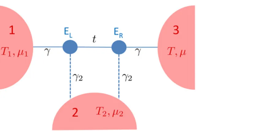
We call t the hopping energy between the dots, and we assume that dot L is coupled to the left lead (1), dot R is coupled to the right lead (3) and that both are coupled to a third lead (2) (see ﬁgure 8). The self energies describing these couplings are:

0 0 0 , 0 0 , 0 0 0 . (43) 1 1 2 2 2 3 3 Σ σ Σ σ σ Σ σ = ⎡ = = ⎣⎢ ⎤ ⎦⎥ ⎡ ⎣ ⎢ ⎤_⎦⎥ ⎡_⎣⎢ ⎤_⎦⎥

In the wide-band approximation, we assume that these quantities are energy-independent and they can be written as purely imaginary numbersσ_i= − i /2γ_i . The self energies thus become:

i i i i 2 0 0 0 , 2 0 0 2 , 0 0 0 2 . (44) 1 1 2 2 2 3 3 Σ γ Σ γ γ Σ γ = − = − − = − ⎡ ⎣ ⎢ ⎢ ⎤ ⎦ ⎥ ⎥ ⎡ ⎣ ⎢ ⎢ ⎢ ⎤ ⎦ ⎥ ⎥ ⎥ ⎡ ⎣ ⎢ ⎢ ⎤ ⎦ ⎥ ⎥

The retarded Greenʼs function of the system is then:

E H E E t t E E E E i t t E E i [ ] 2 2 , (45) L R R L 1 1 2 3 2 1 1 det[ ] 3 2 1 2  Σ σ σ σ σ γ γ γ γ = − − = − − − − − − = = − + + − − − + + − − ⎡ ⎣ ⎢ ⎤_⎦⎥ ⎡ ⎣ ⎢ ⎢ ⎢ ⎢ ⎤ ⎦ ⎥ ⎥ ⎥ ⎥  

Figure 8. Sketch of the double dot model used in the numerical simulations: two quantum dots with a single energy level are connected in series to three fermionic reservoirs 1, 2 and 3. The chemical potential and temperature of reservoir 3 are assumed as the reference valuesμ and T. A two-terminal conﬁguration is obtained in the case in which the coupling to reservoir 2 (equal for both the dots) vanishes (γ = ).₂ 0

(18)

with E E i E E i t det [ ] 2 2 . (46) L R 1 2 3 2 2 γ γ γ γ = ⎜⎛ − + + ⎟ ⎜ − + + ⎟ − ⎝ ⎞ ⎠ ⎛ ⎝ ⎞ ⎠ 

Let us now deﬁne the broadening matrices asΓ_i = i

(

Σ_i − Σ_i†

)

:

0 0 0 , 0 0 , 0 0 0 . (47) 1 1 2 2 2 3 3 Γ γ Γ γ γ Γ γ = ⎡ = = ⎣⎢ ⎤ ⎦⎥ ⎡ ⎣ ⎢ ⎤ ⎦ ⎥ ⎡ ⎣⎢ ⎤ ⎦⎥

The matrix of transmission probability_ij between each pair of reservoirs is then given by the Fisher–Lee formula [39, 45]

Tr . (48)

ij = Γi Γj

†

⎡⎣ ⎤⎦

  

For the system under consideration we obtain

t det [ ] , (49) 13 1 3 2 2 γ γ =  

(

E E

)

t det [ ] R 2 , (50) 12 1 2 2 2 ₃ ₂ 2 ₂ γ γ γ γ = ⎡ − + ⎜ + ⎟ + ⎣ ⎢ ⎛_⎝ ⎞_⎠ ⎤ ⎦ ⎥  

(

E E

)

t det [ ] L 2 . (51) 32 3 2 2 2 ₁ ₂ 2 2 γ γ γ γ = ⎡ − + ⎜ + ⎟ + ⎣ ⎢ ⎛_⎝ ⎞_⎠ ⎤ ⎦ ⎥  

At this point, it is clear that the energy dependence of the transmission matrix cannot be factorized as for the single dot case. This model is hence the simplest in which we can observe finite non-local thermopowers and an increase of both the power and the efficiency of the corresponding thermal machine. Wefind that the behavior of such quantities as functions of the various parameters is qualitatively very similar to the case of the single dot, thus confirming that a third terminal could improve the performance of a quantum machine.

Since in this system all the transport coefficients are different from zero, it is instructive to study the behavior of the generalizedfigures of merit defined in equation (29). Infigure 9we show, in the configuration with only one positive heat flux (J₁Q > ),0 Z T₁₁a (dotted line), Z T₁₁b (dashed line) andZ T₁₁c (full line). We investigate their behavior as a function of the couplingγ₂

and of the total coupling γ. Note that in the two-terminal limit ( 0

2

γ → ) Z T₁₁c reduces to the standard thermoelectricfigure of merit ZT, whileZ T₁₁a and Z T₁₁b tend to zero. When we turn on the interaction with the reservoir 2 (left panel), we notice that thefigure of meritZ T₁₁c decreases, while thefigures of merit Z T₁₁b andZ T₁₁a increase their absolute values. From the behavior as a function of the total couplingγ we can see that in the limit of δ-shaped transmission function (γ → ), the0 figures of merit diverge, leading to the Carnot efficiency, while in the limit of broad transmission window (γ → ∞), all thefigures of merit go to zero and we recover the case of zero efficiency.

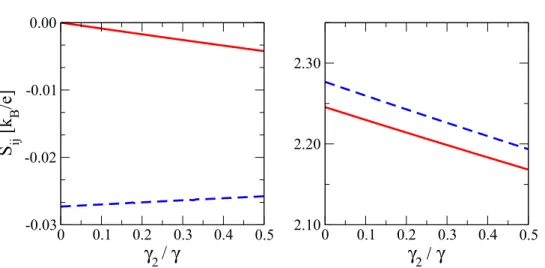
4.2.1. Thermopowers. As mentioned before, the fact that the energy-dependence of the transmission matrix for the double dot cannot be factorized is sufﬁcient to guarantee ﬁnite

(19)

non-local thermopowers, as shown in the left panel ofﬁgure 10. As a function of

2

γ, S₁₂starts from zero, while S₂₁ starts from a ﬁnite value. This different behavior for the two non-local thermopowers is due to the different role played by γ₂ in the two cases. As far as S₁₂ is concerned, when we set a temperature differenceΔT₂ in lead 2, a chemical potential difference

1

Δμ develops in lead 1 to annihilate the current thatﬂows out of the lead 2. When the couplingγ₂

goes to zero, that current goes to zero and so does the chemical potential difference Δμ₁. This argument does not hold forS₂₁, because the temperature difference ΔT₁ is set in lead 1, and

2

γ

does not control the current anymore. Therefore when the coupling γ₂ approaches zero the current still has aﬁnite value, and so the chemical potential difference

2

Δμ needed to annihilate it. Furthermore, the local thermopowers are no more equal, as shown in the right panel of ﬁgure 10.

5. Conclusions

In this paper we have developed a general formalism for linear-response multi-terminal thermoelectric transport. In particular, we have worked out analytical expressions for the

efﬁciency at maximum power in the three-terminal case. By means of two simple

non-interacting models (single- and double-dot), we have shown that a third terminal can be useful to improve the thermoelectric performance of a system with respect to the two-terminal case. Moreover, we have discussed conditions under which non-local thermopowers could be observed. Our analysis could be extended also to cases in which time-reversal symmetry is

broken by a magnetic ﬁeld or including bosonic or superconducting terminals. It is an

interesting open problem to understand in such instances both thermoelectric performance in realistic systems and fundamental bounds on efﬁciency for power generation and cooling.

Figure 9.Various ﬁgures of merit Z T11a (dotted line), Z T

b

11 (dashed line) and Z T

c

11 (full line) as a function of the coupling to the bottom reservoir γ₂ (left panel), and as a function of the total coupling γ (right panel). Parameter values: E_L−μ= −2 k T_B , ER− μ= −20 k TB ,γ = 0.1k TB (left panel) andγ =2 0.5k TB (right panel).

(20)

Acknowledgments

The authors would like to acknowledge H Linke, M Molteni and S Valentini for the useful discussions. This work has been supported by the COST Action MP1209, by the EU project ThermiQ and by MIUR-PRIN: Collective quantum phenomena: from strongly correlated systems to quantum simulators.

Appendix A. Calculation of the transport coefﬁcients and thermopowers

To compute the multi-terminal thermopowers deﬁned in equations (5) and (6) we have to express one of the temperatures as a function of a thermal current. For example let us start from the inversion between X₁T and J₁Q. In the Onsagerʼs formalism this can be expressed as:

(

)

J X J J X J X X L A A X J 0 , (A.1) N T N Q Q T 1 1 2 2 1 1 2 2 1  = − + = − μ μ − _⎜ _⎟ ⎛ ⎝ ⎜ ⎜ ⎜ ⎜⎜ ⎞ ⎠ ⎟ ⎟ ⎟ ⎟⎟ ⎛ ⎝ ⎜ ⎜ ⎜ ⎜ ⎞ ⎠ ⎟ ⎟ ⎟ ⎟ ⎛ ⎝ ⎞⎠ 

where A is a permutation matrix that switches X₁T and J₁Q, X and J are column vectors with components

(

X₁μ, X₁T, X₂μ, X₂T

)

and

(

J₁N, J₁Q, J₂N, J₂Q

)

, respectively, and  is the 4 × 4 identity matrix. Then we obtain:

(

L

)

A A

(

L

)

A B C X J X J X J 0 , (A.2) 1   = − = − = + * * * * − _⎜⎛ _⎟ ⎝ ⎞⎠ ⎛ ⎝ ⎜ ⎞ ⎠ ⎟

Figure 10.(left panel) Non local thermopowers as a function of the couplingγ₂to lead 2. The full red line corresponds to S₁₂= −Δμ Δ₁/ T₂, while the dashed (blue) line corresponds to S21= −Δμ Δ2/ T1. (right panel) Local thermopowers as a function of the coupling γ₂ to lead 2. The full (red) line corresponds to S11= −Δμ Δ1/ T1, while the dashed (blue) line corresponds to S₂₂= −Δμ Δ₂/ T₂. Parameter values as in ﬁgure 9.

(21)

where X* and J* are the vectors X andJafter the action of A−1, that is, with X₁T ↔ J₁Q; B and C are the matrices determined by the product

(

L − 

)

A. We can now deﬁne the thermopower from the following equations:

B C X J X X J X J J X J 0 0 0 . (A.3) Q T N T N Q 1 1 1 2 2 1 1 1 2 2 = − ⇒ = = = = * * μ μ − − ⎛ ⎝ ⎜ ⎜ ⎜ ⎜ ⎞ ⎠ ⎟ ⎟ ⎟ ⎟ ⎛ ⎝ ⎜ ⎜ ⎜ ⎜⎜ ⎞ ⎠ ⎟ ⎟ ⎟ ⎟⎟ 

For this choice of the parameters we have inverted, two different thermopowers can be deﬁned, the non local S₁₂:

S e T eT X X eT L L 1 1 , (A.4) T 12 1 2 1 2 13;34 (2) 13;31 (2) Δμ Δ = − = − = μ

and the local S₂₂:

S e T eT X X eT L L 1 1 . (A.5) T 22 2 2 2 2 14;31 (2) 13;31 (2) Δμ Δ = − = − = μ

The two-terminal limit in which reservoirs 2 and 3 only are connected is obtained after setting in the Onsager matrix L_ij = 0 if i = 1,2 or j = 1,2. In this limit, the previous expressions reduce to: S S eT L L 0, 1 . (A.6) 12 22 34 33 → →

The non-local term goes to zero, while the local one goes to the correct value of the 2-terminal system. The two other terms of these generalized thermopowers are obtained with the inversion of X₂T and J₂Q. Then we can deﬁneS₂₁as the non local quantity, and S₁₁as the local one:

S eT X X eT L L S eT X X eT L L 1 1 , 1 1 . (A.7) T T 21 2 1 13;21 (2) 13;31 (2) 11 1 1 13;32 (2) 13;31 (2) = − = = − = μ μ

In a similar way all the other transport coefﬁcients can be deﬁned, by inverting a generalized force with a current.

Appendix B. Cholesky Decomposition of the three-terminal Onsager matrix

In linear algebra, the Cholesky decomposition [44] is a tool which allows us to write a Hermitian, positive-deﬁnite (or semipositive-deﬁnite) matrix L as a product of a lower triangular matrix D and its conjugate transpose D†:

(22)

L = DD ,† (B.1)

(in particular, if L is real, D† is simply the transpose of D). It turns out that the sign of some quantities deﬁned throughout this work as combinations of products of Onsager coefﬁcients L_ij

can be easily studied by using the Cholesky decomposition on the Onsager matrix L. As an example, by writing D 0 0 0 0 0 0 , (B.2) 11 12 22 13 23 33 14 24 34 44 ρ ρ ρ ρ ρ ρ ρ ρ ρ ρ = ⎛ ⎝ ⎜ ⎜ ⎜ ⎜ ⎞ ⎠ ⎟ ⎟ ⎟ ⎟

it can be shown that the coefﬁcient b and c deﬁned in equation (23) are equal to

(

) (

)

(

)

(

)

(

)

b T c T , , (B.3) 14 2 23 2 33 2 23 24 33 34 2 3 23 2 33 2 22 2 23 2 12 2 23 2 33 2 3 23 2 33 2 ρ ρ ρ ρ ρ ρ ρ ρ ρ ρ ρ ρ ρ ρ ρ ρ = + + + + = + + +

and therefore are non-negative. The coefﬁcient

(

)

(

)

(

)

a T 12 14 23 2 33 2 22 23 23 24 33 34 3 23 2 33 2 ρ ρ ρ ρ ρ ρ ρ ρ ρ ρ ρ ρ = + + + +

instead has an undeﬁned sign. Still one can prove that it is such that the determinant of the matrix M which appears in equation (22) is non-negative. Indeed we have

(

)

(

)

M T det ( ) 14 22 23 12 23 24 12 33 34 , (B.4) 2 6 23 2 33 2 ρ ρ ρ ρ ρ ρ ρ ρ ρ ρ ρ = − + + +

which, together with the positivity of b and c entails that M is semi-positive deﬁnite.

The same procedure can be used to study the sign of the constantsC₁, C₂andC₁₂deﬁned in equations (33), (34), and (35), respectively. As it is shown here below,C₁ and C₂ are always non-negative, whileC₁₂ has an undeﬁned sign:

(

)

(

)

(

)

(

)

(

)

(

)

(

)

(

)

(

)

C C C 2 , 2 , . (B.5) 1 22 33 24 33 23 34 2 23 2 33 2 44 2 22 2 33 2 2 22 33 24 33 23 34 2 23 2 33 2 44 2 24 33 23 34 2 23 2 33 2 44 2 12 22 33 24 33 23 34 2 ₂ 23 2 33 2 44 2 22 33 24 33 23 34 δρ ρ ρ ρ ρ ρ ρ ρ ρ ρ ρ δρ ρ ρ ρ ρ ρ ρ ρ ρ ρ ρ ρ ρ ρ ρ ρ ρ ρ δρ ρ δρ ρ δ ρ ρ ρ ρ ρ ρ ρ ρ ρ = + − + + = + − + + − + + = + − + + − ⎡ ⎣ ⎤⎦ ⎡ ⎣ ⎤⎦

(23)

Appendix C. Scattering approach in linear response: the Onsager coefﬁcients

For a three-terminal conﬁguration, as in the previous sections, we choose the right reservoir 3 as the reference (μ₃ = μ = , T0 ₃ = T), and characterize the problem in terms of the particle/heat currentsﬂowing in linear response between the system and leads 1 (held at μ₁ = μ + Δμ₁ and

T₁= T + ΔT₁) and 2 (held at

2 2

μ = μ + Δμ and T₂ = T + ΔT₂). The Onsagerʼs coefﬁcients are obtained from the linear expansion of the currents J_iN and J_iQ (i=1,2) given by equations (39) and (40). They can be written in terms of the transmission probabilities _ij, i j, ∈ {1, 2, 3}as:

(

)

(

) (

)

(

)

(

)

(

) (

)

(

) (

)

(

)

(

)

(

) (

)

(

)

(

) (

)

(

)

(

)

(

)

(

)

L T h dE f L T h dE f E L L T h dE f L L T h dE f E L L T h dE f E L T h dE f E L L T h dE f E L L T h dE f L T h dE f E L L T h dE f E , ( ) , , ( ) , ( ) , ( ) , ( ) , , ( ) , ( ) , (C.1) E E E E E E E E E E 11 12 13 12 12 13 21 13 12 31 14 12 41 22 2 12 13 23 12 32 24 2 12 42 33 12 23 34 12 23 43 44 2 12 23

∫

μ μ μ μ μ μ μ = − ∂ + = − ∂ − + = = − ∂ − = = − ∂ − − = = − ∂ − + = − ∂ − − = = − ∂ − − = = − ∂ + = − ∂ − + = = − ∂ − +                

where T is the temperature, f denotes the Fermi–Dirac distribution at μ, and ∂_E is the partial derivative with respect to the energy.

C.1. Transmission function of a single-level dot

For a scattering region consisting of a quantum dot with a single energy level, connected to the three-terminal, we can express the transmission function as [38]

( )

(

E E

)

i j , ( ), (C.2) ij i j d 2 2 2 Γ Γ = − + ≠ Γ 

where Γ_i is the contribution to the broadening due to the coupling to lead i, deﬁned by

(

)

i

i i i

Γ = Σ − Σ† , Σ being the self-energy of lead i. In the wide-band limit approximation, we_i

set _i i /2

i

Σ = − γ , where

i

γ does not depend on the energy. Note that this choice leads to the identiﬁcationΓ_i = . Furthermore, at the denominator,γ_i Γ = Γ₁+ Γ₂ + Γ₃ is the total broadening

(24)

due to the coupling to all leads. If we denoteγ₁= ,γ γ₂ = cγ, andγ₃ = dγ the couplings to the three leads, we obtain for the transmissions the values

(

)

(

)

(

)

c E E c d c d E E c d d cd E E c d cd (1 ) 4 , (1 ) 4 , (1 ) 4 . (C.3) d d d 12 2 2 2 ₂ 13 2 2 2 ₂ 23 2 2 2 2 γ γ γ γ γ γ = − + + + ≡ = − + + + ≡ = − + + + ≡      

The Onsager coefﬁcients then read as follows:

L L c d L L c d L c L L c L L L c d L c L L c L L c L d L c L d L c L d ( ), ( ), , , ( ), , , (1 ), (1 ), (1 ), (C.4) 11 0 12 1 13 0 14 1 22 2 23 1 24 2 33 0 34 1 44 2 = + = + = − = − = + = − = − = + = + = + withLn dE

(

f

)

(E ) T h E n

∫

μ = − ∂ −  .

The numerical data shown in section4.1are obtained for d=1, i.e. forγ₁= γ₃ = . The two-γ

terminal conﬁguration corresponds to c = 0 (γ = ), while the coupling to terminal 2 is₂ 0 switched on progressively by increasing c.

References

[1] Mahan G, Sales B and Sharp J 1997 Phys. Today50 42 [2] Majumdar A 2004 Science303 777

[3] Dresselhaus M S, Chen G, Tang M Y, Yang R G, Lee H, Wang D Z, Ren Z F, Fleurial J-P and Gogna P 2007 Adv. Mater.19 1043

[4] Snyder G J and Toberer E S 2008 Nature Mater7 105 [5] Shakouri A 2011 Annu. Rev. Mater. Res.41 399 [6] Dubi Y and di Ventra M 2011 Rev. Mod. Phys.83 131

[7] Benenti G, Casati G, Prosen T and Saito K 2013 arXiv:1311.4430

[8] Jacquet P A 2009 J. Stat. Phys134 709

[9] Entin-Wohlman O, Imry Y and Aharony A 2010 Phys. Rev. B82 115314 [10] Entin-Wohlman O and Aharony A 2012 Phys. Rev. B85 085401

(25)

[11] Jiang J H, Entin-Wohlman O and Imry Y 2012 Phys. Rev. B85 075412 [12] Jiang J H, Entin-Wohlman O and Imry Y 2013 Phys. Rev. B87 205420 [13] Saito K, Benenti G, Casati G and Prosen T 2011 Phys. Rev. B84 201306(R) [14] Horvat M, Prosen T, Benenti G and Casati G 2012 Phys. Rev. E86 052102 [15] Balachandran V, Benenti G and Casati G 2013 Phys. Rev. B87 165419 [16] Sánchez R and Büttiker M 2011 Phys. Rev. B83 085428

[17] Sánchez D and Serra L 2011 Phys. Rev. B84 201307(R) [18] Sothmann B and Büttiker M 2012 Euro Phys. Lett.99 27001

[19] Sothmann B, Sánchez R, Jordan A N and Büttiker M 2012 Phys. Rev. B85 205301 [20] Brandner K, Saito K and Seifert U 2013 Phys. Rev. Lett.110 070603

[21] Brandner K and Seifert U 2013 New J. Phys.15 105003

[22] Bedkihal S, Bandyopadhyay M and Segal D 2013 Eur. Phys. J. B86 506 [23] Benenti G, Saito K and Casati G 2011 Phys. Rev. Lett.106 230602

[24] Yvon J 1955 Proceedings of the International Conference on Peaceful Uses of Atomic Energy (Geneva: United Nations)

[25] Chambadal P 1957 Les Centrales Nucléaires (Paris: Armand Colin) [26] Novikov I I 1958 J. Nucl. Energy7 125

[27] Curzon F and Ahlborn B 1975 Am. J. Phys.43 22 [28] Van den Broeck C 2005 Phys. Rev. Lett.95 190602 [29] Schmiedl T and Seifert U 2008 Europhys. Lett.81 20003

[30] Esposito M, Lindenberg K and Van den Broeck C 2009 Europhys. Lett.85 60010

[31] Esposito M, Kawai R, Lindenberg K and Van den Broeck C 2010 Phys. Rev. Lett.105 150603 [32] Nakpathomkun N, Xu H Q and Linke H 2010 Phys. Rev. B82 235428

[33] Apertet Y, Ouerdane H, Goupil C and Lecoeur Ph 2012 Phys. Rev. B85 033201 [34] Andresen B 2011 Angew. Chem. Int. Ed.50 2690

[35] Machon P, Eschrig M and Belzig W 2013 Phys. Rev. Lett.110 047002

[36] Callen H B 1985 Thermodynamics and an Introduction to Thermostatics 2nd edn (New York: Wiley) [37] de Groot S R and Mazur P 1962 Nonequilibrium Thermodynamics (Amsterdam: North-Holland) [38] Büttiker M 1988 IBM J. Res. Dev.32 63

[39] Datta S 1995 Electronic Transport in Mesoscopic Systems (Cambridge: Cambridge University Press) [40] Imry Y 1997 Introduction to Mesoscopic Physics (Oxford: Oxford University Press)

[41] Mahan G D and Sofo J O 1996 Proc. Natl Acad. Sci. USA93 7436

[42] Humphrey T E, Newbury R, Taylor R P and Linke H 2002 Phys. Rev. Lett.89 116801 [43] Humphrey T E and Linke H 2005 Phys. Rev. Lett.94 096601

[44] Gentle J E 1998 Cholesky factorization Numerical Linear Algebra for Applications in Statistics (Berlin: Springer)