Solar mirrors characterization for concentrating solar power technology

(1)

a.y 2009/2011

Università degli Studi di Catania

Scuola Superiore di Catania

International PhD

in

Energetics

XXIV cycle

S

OLAR MIRRORS CHARACTERIZATION FOR CONCENTRATING SOLAR

POWER TECHNOLOGY

Dott. Ing. Alessandro Patrizio Contino

Coordinator of PhD

Tutor

(2)

2

ABSTRACT

The increasing availability on the market of different types of solar reflectors such as: polymeric film mirrors, aluminum mirrors and thin glass mirrors, together with: the lack of available norms in this area, and a valid methodology to compare the performances of the candidate reflectors; highlights the necessity to conduct a more detailed analysis on these new technologies.

The objective of the present work is to suggest a valuable method to compare the reflectance performance of mirrors, evaluating also their performances in order to assess:

- the most durable to ageing and weathering effects;

- the different reflectance behavior with the variation of the solar incident angle.

.For these reasons the work here proposed was carried out with an experimental apparatus composed by:

- An Agilent Cary 5000 UV/Vis/NIR spectrophotometer to test the different performance of the mirrors at different characterization steps;

- An integrating sphere of 150 mm in diameter (DRA – Diffuse Reflectance Accessory); - A VASRA (Variable Angle Specular Reflection Accessory);

- A UV chamber to accelerate the ageing process;

- A µScan SMS Scatterometer for RMS Roughness and BDSF measurement; - An outdoor bench

The work was completed with two modeling tools:

- An engineering equation solver (Mathcad) to dynamically evaluate the behavior; - A ray tracing software (Soltrace) to evaluate the system’s optical efficiency.

The analysis indicates that the candidate reflectors can be accurately characterized with five fundamental parameters:

a) ρSWH, the solar-weighted hemispherical reflectance; b) ρSWS, the solar-weighted specular reflectance;

c) ρSWS(), the solar weighted specular reflectance function of the variable angle of incidence;

d) BDSF, Bi Directional Scattering Function; e) RMS Roughness

This evaluation will provide a valuable tool, for the companies who want to invest in concentrating solar power technology, to decide whether or not using a candidate reflectors to realize new plants, assessing their performances, their costs, and their durability.

(3)

3 Keywords: Specular Reflectance, Polymeric film reflector, Aluminum reflector, Thin glass reflector, high reflective mirrors, parabolic trough, BSDF, Scatterometer, UV/VIS NIR spectrophotometer, Integrating sphere, CSP, parabolic trough, renewable energy, optical efficiency, UV ageing test solar reflector, Solar Weighted Hemispherical Reflectance, Solar Weighted Specular Reflectance, RMS Roughness, Soltrace®, Mathcad®.

(4)

4

Approved by

Coordinator of Ph.D.: Prof. Alfio Consoli __________________

(5)

5

LIST OF CONTENTS

ABSTRACT ... 2

LIST OF FIGURES ... 10

1. INTRODUCTION ... 21

2. CONCENTRATING SOLAR POWER SYSTEMS... 23

2.1 Technology Description and Status ... 24

2.2 Cost and Potential for Cost Reductions ... 26

2.3 Cost Overview... 26

2.4 Linear Concentrator Systems ... 28

2.5 Parabolic Trough Systems ... 28

2.6 Linear Fresnel Reflector Systems ... 29

2.7 Dish/Engine Systems ... 30

2.8 Solar Concentrator ... 32

2.9 Power Conversion Unit ... 32

2.10 Power Tower Systems ... 33

2.11 Thermal Storage ... 34

2.12 Future R&D Efforts ... 35

3. SPETTROSCOPY ... 37

3.1 Reflection ... 39

3.1.1 Hemispheric Reflectance ... 42

3.2. Transmission ... 45

3.3 Emission ... 49

3.4 Correlation between emissivity and reflectance ... 51

3.5 The Mie theory ... 52

4. INSTRUMENTATION & MEASUREMENTS ... 55

(6)

6

4.1.1 Introduction ... 55

4.1.2. Integrating sphere (Introduction) ... 63

4.1.3 Integrating Sphere (Measuring Sample Reflectance) ... 66

4.1.4 Description of the accessory ... 70

4.1.5 Optics ... 72

4.16 Specifications ... 74

4.1.6 Integrating Sphere Theory ... 75

4.2 VASRA (Variable Angle Specular Reflectance Accessory) ... 96

4.2.1 Specification... 96

4.2.2 Optical Design... 97

4.3 Experimental collection of reflectance data ... 98

4.3.1 Normative references ... 99

4.3.2 Terms and definitions... 100

4.4 Relevance of the reflectance parameter for CSP applications ... 103

4.4.1 Reflective behaviour of solar mirrors ... 103

4.5 Preparation of measurement... 104 4.5.1 Sample preparation ... 104 4.5.2 General ... 104 4.5.3 Cleaning ... 105 4.5.4 Glass mirrors ... 105 4.5.5 Aluminum sheets... 106

4.5.6 Silver polymer films... 106

4.6 Reference mirrors for integrating spheres ... 106

4.7 Measurement procedure ... 106

4.8 Measurement of hemispherical reflectance with spectrophotometer and integrating sphere 107 4.8.1 Configuration of the instrument ... 107

(7)

7

4.8.2 Auto corrections ... 107

4.8.3 Calibration ... 108

4.8.4 Procedure ... 108

4.9 Weighting with standard solar norm spectrum ... 108

4.9.1 Recommended solar norm ... 108

4.9.2 Irradiance spectrum tables ... 109

4.9.3 Solar-weighted hemispherical reflectance ... 110

4.9.4 Solar-weighted specular reflectance ... 121

4.10 Accuracy ... 121

5. REFLECTANCE MEASUREMENTS ... 123

5.1 DRA (Diffuse Reflectance Accessory) Integrating Sphere ... 123

5.1.1 Thin Glass Mirrors ... 123

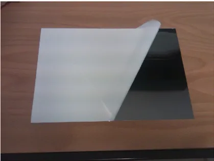
5.1.2 Aluminum Mirrors ... 129

5.1.3 Polymeric film mirrors ... 135

5.2 VASRA Reflectance Measurements ... 143

5.2.1 Thin Glass Mirrors ... 146

5.2.2 Aluminum Mirrors ... 151

5.3 UV Accelerated Ageing Tests... 163

5.3.1 Thin glass mirrors ... 172

5.3.2 Aluminum mirrors... 177

5.3.3 Polymeric film mirror ... 181

5.4 Outdoor exposure measurements ... 185

5.4.2 Aluminum mirror ... 192

(8)

8

5.5 Reflectance measurement after one month (Scatterometer) ... 199

5.5.3 Polymeric mirror ... 205

5.6 Comparison between the scatterometer measurement after one month ... 207

5.7 Reflectance measurement after one month (Spectrophotometer) ... 210

5.7.1 Thin Glass mirrors ... 210

6. MODELING ... 225

6.1 Mathcad® ... 225

6.1.1 Direct Normal Insolation ... 225

6.1.2 Angle of incidence ... 226

6.1.3 Optical Efficiency and HCE Efficiency ... 232

6.1.4 Incidence Angle Modifier (IAM) ... 234

6.1.5 Row Shadowing and End Losses ... 235

6.1.6 Solar Irradiation Absorption ... 238

6.1.8 Aluminum mirrors ... 244

6.2 Soltrace® ... 252

6.2.1 Defining the Sun ... 255

6.2.2 Defining Optical Geometry ... 257

6.2.3 Defining System Geometry ... 259

6.2.4 Tracing Overview ... 263

(9)

9

6.2.8 Polymeric Film mirrors ... 287

6.3 Comparison between Mathcad and Soltrace models ... 296

7. ENHANCING THE MODEL ... 303

7.2 Receiver Heat Loss ... 303

7.3 Analytical Heat Loss Derivation ... 303

7.3.1 Linear Regression Heat Loss Model ... 304

7.3.2 Solar Field Piping Heat Losses ... 308

7.4 Heat Transfer Fluid Energy Gain ... 309

7.5 Heat losses evaluation ... 309

7.6 Results ... 317

7.6.1 Thin glass ... 317

7.7 Result improvement ... 347

8. CONCLUSION ... 352

(10)

10

LIST OF FIGURES

Figure 2. 1 A linear concentrator power plant using parabolic trough collectors ... 29

Figure 2. 2 A linear Fresnel reflector power plant ... 30

Figure 2. 3 SES Dish/Stirling system ... 31

Figure 2. 4 A dish/engine power plant. ... 32

Figure 2. 5 A power tower power plant. ... 33

Figure 3. 1 Typical material absorption process ... 37

Figure 3. 2 Spectrum division ... 38

Figure 3. 3 Optics Angles ... 39

Figure 3. 4 Bi-directional reflectance ... 40

Figure 3. 5 Hemispheric reflectance ... 42

Figure 3. 6 Transmission through a material ... 45

Figure 3. 7 Schematic diagram of an emission measurement ... 51

Figure 4. 1 Spectrophotometer Agilent Cary 5000 ... 55

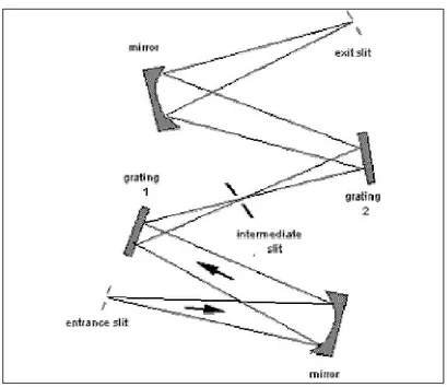
Figure 4. 2 Spectrophotometer optics: a) schematic diagram ... 56

Figure 4. 3 Spectrophotometer light sources ... 57

Figure 4. 4 Spectrophotometer sample holder, one for the reference beam and the other for the sample beam ... 58

Figure 4. 5 Diffraction grating geometry ... 60

Figure 4. 6 Overlap of the spectral orders ... 61

Figure 4. 7 Grating mounting on a dual monochromator ... 62

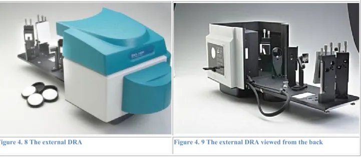
Figure 4. 8 The external DRA ... 63

Figure 4. 9 The external DRA viewed from the back ... 63

Figure 4. 10 Optical geometry of an integrating sphere ... 65

Figure 4. 11 PTFE reference disk ... 66

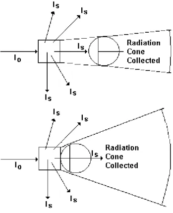
Figure 4. 12 Collection of scattered light by an integrating sphere. Io = incident light, Is = scattered light ... 67

Figure 4. 13 Some of the wide-angle scatter is lost when there is a space between the sample and the sphere wall ... 68

Figure 4. 14 Some of the wide-angle reflection is intercepted by the sphere wall ... 68

(11)

11

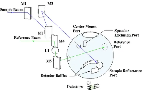
Figure 4. 16 A schematic view of the external DRA ... 71

Figure 4. 17 The optical design of the external DRA ... 71

Figure 4. 18 Mirror M1 ... 72

Figure 4. 23 Radiation exchange between two surfaces ... 75

Figure 4. 24 Angles relation between the two mentioned surfaces ... 76

Figure 4. 25 Schematics of the inside of the sphere... 77

Figure 4. 26 Diagram of the magnitude of the sphere multiplier ... 79

Figure 4. 27 Diagram of the magnitude of radiance vs numbers of reflection ... 81

Figure 4. 28 Relative radiance plotted on different values of diameter ... 83

Figure 4. 29 Spectral reflectance of most used internal coatings... 84

Figure 4. 30 Schematics on measurement of reflectance on the detector area ... 87

Figure 4. 31 Schematics on measurement of reflectance on the detector area ... 87

Figure 4. 32 measurement of omnidirectional flux ... 90

Figure 4. 33 measurement of unidirectional flux ... 90

Figure 4. 34 measurement of neither Omnidirectional or Unidirectional flux Detectors ... 91

Figure 4. 35 Human eye spectral response ... 91

Figure 4. 36 The optical design of the Variable Angle Specular Reflectance Accessory ... 97

Figure 4. 37 The beam profiles at 20° ... 98

Figure 4. 38 The beam profiles at 70° ... 98

Figure 4. 39 Diffuse reflectance ... 100

Figure 4. 40 Perfect specular reflection Figure 4. 41 Specular reflection with offset ... 101

Figure 4. 42 Approximated reflection distribution for non-ideal specular mirror materials ... 104

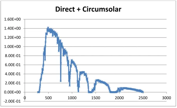
Figure 4. 43 Direct + Circumsolar spectrum calculated with SMARTS model in a clear sky day at AM 1.5 ... 109

Figure 5. 1 Reflector type TG1 Figure 5. 2 Reflector type TG2 ... 124

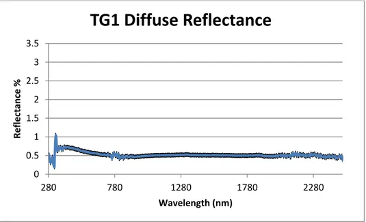
Figure 5. 3 TG1 Reflectance Measurements ... 124

Figure 5. 4 Diffuse Reflectance ... 125

Figure 5. 5 Specular Reflectance ... 126

(12)

12

Figure 5. 9 Solar Weighted Hemispherical Reflectance ... 129

Figure 5. 10 Solar Weighted Specular Reflectance ... 129

Figure 5. 11 Aluminum mirror AL1 Figure 5. 12 Aluminum mirror AL2 ... 130

Figure 5. 13 Reflectance Measurements ... 131

Figure 5. 16 TG2 Reflectance measurement ... 132

Figure 5. 21 PF1 mirror... 135

Figure 5. 22 PF1 Global+Diffuse ... 136

Figure 5. 25 PF2 Global+Diffuse ... 138

Figure 5. 30 Summary of the different Solar Weighted Hemispherical Reflectance ... 141

Figure 5. 31 Summary of the different Solar Weighted Specular Reflectance ... 141

Figure 5. 32 VASRA Reflectance Measurements for TG1 Samples ... 146

Figure 5. 33 VASRA Reflectance measurements for TG2 Samples ... 147

Figure 5. 34 Solar Weighted Specular Reflectance at different angles of incidence for TG1 Samples: a=20°,b=25°,c=30°,d=35°,e=40°,f=45°,g=50°,h=55°,l=60°,m=65°,n=70° ... 148

Figure 5. 35 Solar Weighted Specular Reflectance at different angles of incidence for TG2 Samples: a=20°,b=25°,c=30°,d=35°,e=40°,f=45°,g=50°,h=55°,l=60°,m=65°,n=70° ... 149

Figure 5. 36 Reflectance Vs Angle of Incidence ... 149

(13)

13

Figure 5. 39 Comparison between the two thin glass mirrors ... 151

Figure 5. 40 VASRA Reflectance Measurements for AL1 Samples ... 152

Figure 5. 41 VASRA Reflectance measurements for TG2 Samples ... 153

Figure 5. 42 Solar Weighted Specular Reflectance at different angles of incidence for AL1 Samples: a=20°,b=25°,c=30°,d=35°,e=40°,f=45°,g=50°,h=55°,l=60°,m=65°,n=70° ... 154

Figure 5. 43 Solar Weighted Specular Reflectance at different angles of incidence for AL2 Samples: a=20°,b=25°,c=30°,d=35°,e=40°,f=45°,g=50°,h=55°,l=60°,m=65°,n=70° ... 154

Figure 5. 46 TG1 Mirror Vs TG2 Mirror ... 156

Figure 5. 47 Comparison between the two aluminum mirrors ... 157

Figure 5. 48 VASRA Reflectance Measurements for PF1 Samples ... 158

Figure 5. 49 Solar Weighted Specular Reflectance at different angles of incidence for PF Samples: a=20°,b=25°,c=30°,d=35°,e=40°,f=45°,g=50°,h=55°,l=60°,m=65°,n=70° ... 159

Figure 5. 50 Reflectance Vs Angles of incidence ... 159

Figure 5. 51 PF2 VASRA measurements ... 160

Figure 5. 52 Reflectance vs Angles of incidence ... 161

Figure 5. 53 Relative reflectance comparison ... 161

Figure 5. 54 Comparison between the two polymeric mirrors ... 162

Figure 5. 55 Comparison graph between all the mirrors tested ... 162

Figure 5. 56 UV Chamber ... 163

Figure 5. 57 Ultramed 2000 lamp ... 164

Figure 5. 58 LP UVA & LP UVB probes ... 164

Figure 5. 59 LP UVA 01 typical spectral response... 166

Figure 5. 60 LP UVB 01 typical spectral response ... 167

Figure 5. 61 Positions of UVA + UVB measurements ... 168

Figure 5. 62 The wood board inside the UV chamber ... 171

Figure 5. 63 Schematic and real system constructed at the laboratory ... 171

Figure 5. 64 TG1 global and diffuse reflectance after the treatment in the UV chamber ... 172

Figure 5. 65 Specular reflectance spectrum comparison ... 173

Figure 5. 66 Diffuse reflectance comparison ... 173

Figure 5. 67 Solar weighted hemispherical (ρSWH) and specular (ρSWS) reflectance ... 174

(14)

14

Figure 5. 69 Specular reflectance comparison ... 175

Figure 5. 71 Solar weighted hemispherical (ρSWH) and specular (ρSWS) reflectance ... 176

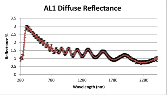
Figure 5. 72 AL1 spectral response ... 177

Figure 5. 73 AL1 specular reflectance ... 178

Figure 5. 75 Solar weighted hemispherical and specular reflectance ... 179

Figure 5. 76 AL2 spectral response ... 179

Figure 5. 77 AL2 specular reflectance ... 180

Figure 5. 79 Comparison between the before and after condition for solar weighted hemispherical and specular reflectance ... 181

Figure 5. 80 PF1 Spectral response ... 182

Figure 5. 81 Specular reflectance variation ... 182

Figure 5. 83 Comparison of Solar weighted hemispherical and specular reflectance at time 0 and after the UV exposure ... 183

Figure 5. 84 Solar weighted hemispherical reflectance in the condition 0 and after one year of UV exposure ... 184

Figure 5. 85 Solar weighted specular reflectance in the condition 0 and after one year of UV exposure ... 184

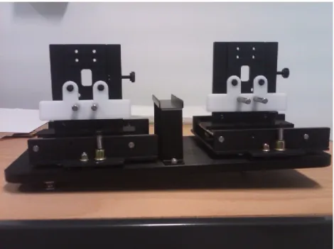
Figure 5. 86 Aluminum structure for outdoor exposure ... 185

Figure 5. 87 External bench for outdoor exposure test ... 186

Figure 5. 88 SMS Scatterometer ... 187

Figure 5. 89 Instrument technical information ... 187

Figure 5. 90 Reference dielectric mirror ... 188

Figure 5. 91 Certificate of calibration and reference mirror value ... 188

Figure 5. 92 Reflectance at 25° (primary axis) and RMS Roughness (Secondary axis) ... 189

Figure 5. 93 BDSF at (0,0) and (50,180) for the TG1 sample ... 190

(15)

15

Figure 5. 99 BDSF at (0,0) and (50,180) for the AL2 sample ... 195

Figure 5. 103 BDSF at (0,0) and (50,180) for the AL2 sample ... 199

Figure 5. 104 The mirror samples after one month of outdoor exposure ... 200

Figure 5. 105 Reflectance and RMS roughness values ... 201

Figure 5. 106 BDSF (0,0) and BDSF (50,180) values ... 201

Figure 5. 115 Comparison between the BDSF (0,0) and (50,180) at time 0 and after one month of outdoor exposure ... 207

Figure 5. 116 Reflectance values at 0 time and after 1 month of outdoor exposure ... 208

Figure 5. 117 RMS Roughness at 0 time and after 1 month of outdoor exposure ... 209

Figure 5. 118 TG1 spectral response after one month of outdoor exposure ... 211

Figure 5. 119 TG2 specular spectral response at 0 time and after one month of outdoor exposure 211 Figure 5. 120 Diffuse reflectance comparison between the sample in "before" and "after" condition ... 212

Figure 5. 121 Global + diffuse reflectance after one month of outdoor exposure ... 212

Figure 5. 122 Specular reflectance comparison between the "before" and "after" condition ... 213

Figure 5. 123 Diffuse reflectance comparison between the "before" and "after" condition ... 213

Figure 5. 124 Comparison between the solar weighted hemispherical reflectance for TG1 and TG2 sample in the "before" and "after" condition ... 214

Figure 5. 125 Comparison between the solar weighted specular reflectance for TG1 and TG2 sample in the "before" and "after" condition ... 215

(16)

16 Figure 5. 126 Global + diffuse reflectance spectral response after one month of outdoor exposure

... 216

Figure 5. 129 Global + diffuse reflectance spectral response after one month of outdoor exposure ... 217

Figure 5. 132 Comparison between the solar weighted hemispherical reflectance for AL1 and AL2 sample in the "before" and "after" condition ... 219

Figure 5. 133 Comparison between the solar weighted specular reflectance for AL1 and AL22 sample in the "before" and "after" condition ... 220

Figure 5. 134 Global + diffuse reflectance spectral response after one month of outdoor exposure ... 221

Figure 5. 137 The solar weighted hemispherical reflectance for PF1 sample in the "before" and "after" condition ... 222

Figure 5. 138 Solar weighted specular reflectance for the PF1 mirror ... 223

Figure 5. 139 Solar weighted hemispherical reflectance at 0 time and after one month of outdoor exposure ... 223

Figure 5. 140 Solar weighted specular reflectance at 0 time and after one month of outdoor exposure ... 224

Figure 6. 1 Direct Normal Insolation as measured in Catania during the year 2009 ... 226

Figure 6. 2 Angle of incidence between the collector normal and the beam radiation ... 227

Figure 6. 3 Declination angle due to Earth's tilt ... 227

Figure 6. 4 Shows the variation of the declination angle throughout the year ... 228

Figure 6. 5 Equation of time vs month of the year ... 229

Figure 6. 6 Solar altitude angles versus time, on June 21 and December 21 of the year, for Catania ... 230

Figure 6. 7 DNI and DNI cos () in Catania on June 21 ... 231

(17)

17 Figure 6. 9 Collector tracking through morning, showing digression of collector shading as the day

progresses ... 236

Figure 6. 10 RowShadow (Weff/Wh) versus time of day, for June 21 and December 21 ... 237

Figure 6. 11 End losses from an HCE ... 237

Figure 6. 12 End Losses versus incidence angle () ... 238

Figure 6. 13 Hourly average flux values collected from the HCE with the TG1 mirror ... 242

Figure 6. 14 Hourly average flux values collected from the HCE with the TG2 mirror ... 243

Figure 6. 15 Comparison between TG1 and TG2 mirrors ... 244

Figure 6. 16 Hourly average flux values collected from the HCE with the AL1 mirror ... 245

Figure 6. 17 Hourly average flux values collected from the HCE with the A12 mirror ... 247

Figure 6. 19 Hourly average flux values collected from the HCE with the PF1 mirror ... 249

Figure 6. 20 Hourly average flux values collected from the HCE with the PF2 mirror ... 250

Figure 6. 22 Comparison between all the typologies of mirrors ... 252

Figure 6. 23 Soltrace® coordinate system ... 254

Figure 6. 24 Generation of ( x, y, z ) system from the ( x, y, z ) system after translation of origin 254 Figure 6. 25 Defining the Sun Shape and Position ... 256

Figure 6. 26 A glass plane is actually constructed from two separate elements ... 258

Figure 6. 27 Illustration of surface slope and surface specularity error ... 259

Figure 6. 28 Optical geometry definition input page ... 259

Figure 6. 29 The trace setup parameters ... 263

Figure 6. 30 Soltrace model implemented on Google Sketch Up ... 266

Figure 6. 31 Soltrace geometric simulation ... 266

Figure 6. 32 100 sun rays hitting the parabolic surface ... 267

Figure 6. 33 100 sun rays hitting the heat collector element ... 268

Figure 6. 34 Flux collected on the receiver 2D ... 269

Figure 6. 35 Flux collected on the receiver 3D ... 269

Figure 6. 36 Average flux collected on the 172th day for the TG1 mirror ... 274

Figure 6. 37 Average flux collected on the 172th day for the TG2 mirror ... 277

Figure 6. 38 Comparison between the flux collected from TG1 and TG2 mirrors ... 278

(18)

18

Figure 6. 40 Average flux collected on the 172th day for the AL2 mirror ... 286

Figure 6. 41 Comparison between the flux collected from AL1 and AL2 mirrors ... 287

Figure 6. 42Average flux collected on the 172th day for the PF1 mirror ... 291

Figure 6. 43 Average flux collected on the 172th day for the PF2 mirror ... 295

Figure 6. 44 Comparison between the flux collected from PF1 and PF2 mirrors ... 296

Figure 6. 45 Comparison between TG1 Model and TG1 Soltrace ... 297

Figure 6. 46 Comparison between TG2 Model and TG2 Soltrace ... 298

Figure 6. 47 Comparison between AL1 Model and AL1 Soltrace ... 299

Figure 6. 48 Comparison between AL2 Model and AL2 Soltrace ... 300

Figure 6. 49 Comparison between PF1 Model and PF1 Soltrace ... 301

Figure 6. 50 Comparison between PF2 Model and PF2 Soltrace ... 302

Figure 7. 1 Heat transfer mechanisms acting on HCE surfaces ... 304

Figure 7. 2 Dependence of Heat Losses on the Heat Transfer Fluid in air annulus condition ... 310

Figure 7. 3 Values of Heat losse on the 172th day varying the HTF temperature in air condition . 310 Figure 7. 4 Dependence of Heat Losses on the Heat Transfer Fluid in vacuum annulus condition 311 Figure 7. 5 Values of Heat losses on the 172th day varying the HTF temperature in vacuum condition... 311

Figure 7. 6 Variation of Heat losses for TG1 reflectance value at 290°C=(12,j) and at 390°C=(17,j) in vacuum and lost vacuum condition ... 312

Figure 7. 7 Values of Heat Losses in air and vacuum condition for TG1 mirror ... 312

Figure 7. 8 Variation of Heat losses for TG2 reflectance value at 290°C=(12,j) and at 390°C=(17,j) in vacuum and lost vacuum condition ... 313

Figure 7. 9 Values of Heat Losses in air and vacuum condition for TG2 mirror ... 313

Figure 7. 10 Variation of Heat losses for AL1 reflectance value at 290°C=(12,j) and at 390°C=(17,j) in vacuum and lost vacuum condition ... 314

Figure 7. 11 Values of Heat Losses in air and vacuum condition for AL1 mirror ... 314

Figure 7. 12 Variation of Heat losses for AL2 reflectance value at 290°C=(12,j) and at 390°C=(17,j) in vacuum and lost vacuum condition ... 314

Figure 7. 13 Values of Heat Losses in air and vacuum condition for AL2 mirror ... 315

Figure 7. 14 Variation of Heat losses for PF1 reflectance value at 290°C=(12,j) and at 390°C=(17,j) in vacuum and lost vacuum condition ... 315

(19)

19 Figure 7. 16 Variation of Heat losses for PF2 reflectance value at 290°C=(12,j) and at 390°C=(17,j) in vacuum and lost vacuum condition ... 316 Figure 7. 17 Values of Heat Losses in air and vacuum condition for PF2 mirror ... 316 Figure 7. 18 Value of total irradiance absorbed (Qabs), Total irradiance absorbed in vacuum condition (Qtotcollvac), Total irradiance absorbed in air condition (Qtotcollair) [W/m2] for the TG1 mirror ... 318 Figure 7. 19 Irradiance absorbed in different wind speed condition for the TG1 mirror ... 319 Figure 7. 20 Comparison along the year of the values of the 0.0 m/s wind speed and the different wind speed in vacuum and air condition for the TG1 mirror ... 320 Figure 7. 21 Values of yearly collected irradiance at different wind speed and in air or vacuum condition... 321 Figure 7. 22 Value of total irradiance absorbed (Qabs), Total irradiance absorbed in vacuum condition (Qtotcollvac), Total irradiance absorbed in air condition (Qtotcollair) [W/m2] for the TG2 mirror ... 323 Figure 7. 23 Irradiance absorbed in different wind speed condition for the TG2 mirror ... 324 Figure 7. 24 Comparison along the year of the values of the 0.0 m/s wind speed and the different wind speed in vacuum and air condition for the TG2 mirror ... 325 Figure 7. 25 Values of yearly collected irradiance at different wind speed and in air or vacuum condition... 326 Figure 7. 26 Value of total irradiance absorbed (Qabs), Total irradiance absorbed in vacuum condition (Qtotcollvac), Total irradiance absorbed in air condition (Qtotcollair) [W/m2] for the AL1 mirror ... 328 Figure 7. 27 Irradiance absorbed in different wind speed condition for the AL1 mirror ... 329 Figure 7. 28 Comparison along the year of the values of the 0.0 m/s wind speed and the different wind speed in vacuum and air condition for the AL1 mirror ... 330 Figure 7. 29 Values of yearly collected irradiance at different wind speed and in air or vacuum condition... 331 Figure 7. 30 Value of total irradiance absorbed (Qabs), Total irradiance absorbed in vacuum condition (Qtotcollvac), Total irradiance absorbed in air condition (Qtotcollair) [W/m2] for the AL2 mirror ... 333 Figure 7. 31 Irradiance absorbed in different wind speed condition for the AL2 mirror ... 334 Figure 7. 32 Comparison along the year of the values of the 0.0 m/s wind speed and the different wind speed in vacuum and air condition for the AL2 mirror ... 335

(20)

20 Figure 7. 33 Values of yearly collected irradiance at different wind speed and in air or vacuum condition... 336 Figure 7. 34 Value of total irradiance absorbed (Qabs), Total irradiance absorbed in vacuum condition (Qtotcollvac), Total irradiance absorbed in air condition (Qtotcollair) [W/m2] for the PF1 mirror ... 338 Figure 7. 35 Irradiance absorbed in different wind speed condition for the PF1 mirror ... 339 Figure 7. 36 Comparison along the year of the values of the 0.0 m/s wind speed and the different wind speed in vacuum and air condition for the PF1 mirror ... 340 Figure 7. 37 Values of yearly collected irradiance at different wind speed and in air or vacuum condition... 341 Figure 7. 38 Value of total irradiance absorbed (Qabs), Total irradiance absorbed in vacuum condition (Qtotcollvac), Total irradiance absorbed in air condition (Qtotcollair) [W/m2] for the PF2 mirror ... 343 Figure 7. 39 Irradiance absorbed in different wind speed condition for the PF2 mirror ... 344 Figure 7. 40 Comparison along the year of the values of the 0.0 m/s wind speed and the different wind speed in vacuum and air condition for the PF2 mirror ... 345 Figure 7. 41 Values of yearly collected irradiance at different wind speed and in air or vacuum condition... 346 Figure 7. 42 Collected energy values along the year between the different mirrors with constant reflectance ... 348 Figure 7. 43 Collected energy values along the year between the different mirrors with variable reflectance ... 349 Figure 7. 44 Values of total energy collected along the year in air in annulus condition for all the typologies of mirrors ... 349 Figure 7. 45 Values of total energy collected along the year in air in annulus condition for all the typologies of mirrors ... 350 Figure 7. 46 Values of total energy collected along the year with vacuum in annulus condition for all the typologies of mirrors ... 351

(21)

21

1. INTRODUCTION

The solar concentrating technology is far well known; during the eighties it had a great development due to the incentives given by the US government to develop an alternative source of energy capable of supplying enough power to face a possible energy crisis, therefore the SEGS plants were built.

Successively the US government discontinued the incentives and all the efforts done to build and develop these types of plants had to cease as well.

In 2006 the US congress has given the go-ahead with a new flow of incentives to build and develop new CSP plants with different technology. As a result, other countries such as Spain, Italy and Israel started to build and developed such plants.

All of the new plants were built with the same mirror technology as they were in the 80’s, with thick glass mirrors.

They had an excellent reflectance but also great costs, not only for the product itself but also for all the logistics connected to the transportation, installation and maintenance.

As it was expected, new technologies were used to obtain mirrors with a high reflectance factor, easy bending and molding and low weight.

All of these characteristics lead the market to diffuse three different technologies that could cope with the needs mentioned above:

 Thin glass mirrors;  Aluminum mirrors;  Polymeric film mirrors.

The objective of the research here proposed is to better understand the optical behavior of these new technologies, with the evaluation of their specular reflectance near the normal angle (6°), their specular reflectance at different angles of incidence (from 20° to 70°) and after an UV ageing process (able to irradiate the sample with a UV dose equal to a year of outdoor exposure at the Catania latitude) and an outdoor exposure to evaluate the soiling effects on reflectance.

Each of these reflectors appear to possess different characteristics that are not fully described in the commercial brochure, sometimes obtained with a non-precise methodology or worse, obtained with a non-precise instrumental apparatus.

To cope with this lack of information the companies concentrating on building solar power plants have to be able to decide whether to use a material or not.

(22)

22 Distinguishing between a good or a less good material such as mirrors (which is the heart of the entire project) is the key to building new and less expensive plants and can be critical for the initial cost assessment and the maintenance costs during the power plant’s lifespan.

A good material will maintain the optical performances during the entire operational life, will have a good mechanical resistance, have a good weatherability and very high shape accuracy, furthermore it will be light weight, is easy to handle and possesses the quality to be produced in large sizes.

To achieve reliable results in research, different steps were necessary to conduct a measurement campaign with a CARY 5000 UV/VIS NIR spectrophotometer for the reflectance measurements (Chapter 5) in the optical and geometrical study of the systems with two modeling software tools: Mathcad and Soltrace (Chapter 6).

The results (Chapter 7) were used to obtain a quantitative analyses of the energy reflected from the mirrors and absorbed from the Heat Collector Element, maintaining firstly a constant reflectance of the mirrors and then introducing the VASRA experimental results inside the model to simulate the quantity of DNI reflected throughout a year, considering the contribution that the increase of mirrors reflectance show when varying the incidence angle.

(23)

23

2. CONCENTRATING SOLAR POWER SYSTEMS

Concentrating Solar Power (CSP) plants use all the technologies applied to transform sunlight into high-temperature heat and thus converting such heat into electrical energy. The general principle of a CSP plant entails using mirrors to concentrate the sun’s rays on a fluid that vaporizes. The heat from this fluid is transferred into a heat exchanger to a water-steam cycle, which drives a turbine and a generator to generate electricity. The most widespread technology in the CSP sector is a CSP plant based on cylindrical -parabolic mirror technology (also called solar trough plants) with capacities ranging from 50 to 300 MW. Cylindrical-parabolic mirrors concentrate the sun’s rays on an absorber tube containing a heat-transfer fluid that can be heated to temperatures of around 400°C and generate electricity based on heat transfer to a conventional water-steam cycle. Some plants are equipped with storage systems enabling unused, surplus energy to be stored in the form of heat in molten salt or some other phase-changing material.

The plant can then draw on the stored heat to generate electricity after sunset. Spain’s Andasol 1 plant, for example, currently uses this system to operate for an additional 7½ hours every day. Alternatively, solar power is harnessed in 10 to 50 MW-capacity solar tower CSP plants that use heliostats – huge, almost flat mirrors over 100 m2 in surface area. They are arranged in large numbers (up to hundreds) to concentrate the sun’s rays on a point at the top of a tower, heating the heat-transfer fluid (generally a salt) up to as much as 600°C.

Its designed storage capacity is for up to 15 hours which should support almost round-the-clock production, and enable the plant to supplement electricity generation based on fossil fuels or nuclear energy. There are other technologies in the stage of development and demonstration that are not yet used on an industrial scale. For instance, Fresnel linear collectors that are a variant on a CSP plant based on cylindrical-parabolic mirror technology, which instead of using a trough-shaped mirror, have sets of small flat mirrors arranged in parallel and longitudinally on an incline. Furthermore, the absorber tube that concentrates the rays is stationary and the mirrors follow the course of the sun. The fluid is heated to a temperature of up to 450°C.

Development is under way on larger (150-MW and more) plants, but they are outside of Europe. Another alternative technology is the dish Stirling system, based on a dish-shaped concentrator (comprising parabolic mirrors) to capture the sunlight and focus it on a receiver at the focal point of

(24)

24 the parabolic dish. The parabolic dish system, which tracks the sun, uses a gas (helium or hydrogen) that is heated in the receiver to temperatures in excess of 600°C to drive a Stirling engine coupled with a generator. The capacity of these units is limited to 10–25 kW, which will meet isolated production needs. Alternatively, parabolic dish CSP plants may be built as large-scale plants with thousands of parabolic dishes grouped together on a single site. Two projects with an aggregate capacity of 1.4 GW are under construction in the United States, but no industrial-scale ventures have been identified in Europe.

2.1 Technology Description and Status

There are three types of concentrating solar power (CSP) technology: trough, parabolic-dish and power tower.1_{Trough and power tower technologies apply primarily to large, central power} generation systems, although trough technology can also be used in smaller systems for heating and cooling and for power generation.

The systems use either thermal storage or back-up fuels to offset solar intermittency and thus to increase the commercial value of the energy produced.

The conversion path of concentrating solar power technologies relies on four basic elements: concentrator, receiver, and transport-storage and power conversion.

The concentrator captures and concentrates solar radiation, which is then delivered to the receiver. The receiver absorbs the concentrated sunlight, transferring its heat to a working fluid. The transport-storage system passes the fluid from the receiver to the power-conversion system; in some solar-thermal plants a portion of the thermal energy is stored for later use.

The inherent advantage of CSP technologies is their unique capacity for integration into conventional thermal plants. Each technology can be integrated in parallel as “a solar burner” to a fossil burner into conventional thermal cycles. This makes it possible to provide thermal storage or fossil fuel backup firm capacity without the need of separate back-up power plants and without disturbances to the grid.

With a small amount of supplementary energy from natural gas or any other fossil fuel, solar thermal plants can supply electric power on a steady and reliable basis.

(25)

25 Thus, solar thermal concepts have the unique capability to internally complement fluctuating solar burner output with thermal storage or a fossil back-up heater.

The efficiency and cost of such combined schemes, however, can be significant.

Current costs are about USD 0.10 per kWh and are expected to rise to about USD 0.72 per kWh by 2050. This technology relies on small-scale gas-fired power plants with low efficiency (40–45%), compared to 500-MW centralized plants with efficiencies of 60%. If the efficiency loss is allocated to the hybrid scheme, the economics would be less encouraging.

Fresh impetus was given to solar thermal-power generation by a Spanish law passed in 2004 and revised in 2005. The revised law provides for a feed-in-tariff of approximately EUR 0.22 (USD 0.27) per kWh for 500 MW of solar thermal electricity.

In several states in the United States and in other countries, the regulatory framework for such plants is improving. At present, solar plant projects are being developed in Spain (50 MW), in Nevada in the United States (68 MW) and elsewhere.

Two U.S. plants will also be constructed in southern California under the state’s Renewable Portfolio Standard. A 500 MW solar thermal plant, expected to produce 1,047 GWh, is due for completion in 2012.

There is a current trend toward combining a steam-producing solar collector and a conventional natural gas combined-cycle plant. Projects in Algeria and Egypt, currently at the tendering stage, will combine a solar field with a combined-cycle plant. There are also plans to add a solar field to an existing coal plant in Australia.

On a long-term basis, the direct solar production of energy in transportable chemical fuels, such as hydrogen, also holds great promise.

(26)

26

2.2 Cost and Potential for Cost Reductions

Since concentrating solar power uses direct sunlight, the best conditions for this technology are in arid or semi-arid climates, including Southern Europe, Northern and Southern Africa, the Middle East, Western India, Western Australia, the Andean Plateau, Northeastern Brazil, Northern Mexico, and the Southwestern United States. The cost of concentrating solar power generated with up-to-date technology at superior locations is between USD 0.10 and USD 0.15 per kWh. CSP technology is still too expensive to compete in domestic markets without subsidies.

The goal of ongoing RD&D is to reduce the cost of CSP systems to USD 0.05–USD 0.08 per kWh within 10 years and to below USD 0.05 in the long term.

Improved manufacturing technologies are needed to reduce the cost of key components, especially for first plant applications where economies of scale are not yet available. Field demonstration of the performance and reliability of Stirling engines are critical.

The European Commission (EC) has undertaken a coordination activity, called the European Concentrated Solar Thermal Road-mapping (ECOSTAR), to harmonize the fragmented research methodology previously in place in Europe, which previously led to competing approaches on how to develop and implement CSP technology. Cost-targeted innovation approaches, as well as continuous implementation of this technology, are needed to realize cost-competitiveness in a timely manner.

2.3 Cost Overview

There is a wide range of costs for each renewable technology due mainly to varying resource quality and to the large number of technologies within each category. Investment includes all installation costs, including those of some demonstration plants in certain categories. Discount rates vary across regions.

Because of the wide range in costs, there is no specific year or CO2 price level for which a renewable energy technology can be expected to become competitive.

A gradual increase in the penetration of renewable energy over time is more likely.

Energy policies can speed up this process by providing the right market conditions and to accelerate deployment so that costs can be reduced through technology learning.

(27)

27 Technology learning in bioenergy systems has been studied using experiences in Denmark, Finland, and Sweden (Junginger M et al, 2005) (al J. M., 2005). In the supply chain, learning rates for wood fuel-chips are 12–15%. For energy conversion in biogas or fluidized bed boiler plants, available data are much more difficult to interpret. An average learning rate of 5% for energy-producing plants appears to be a reasonable average estimate.

Technology learning is a key phenomenon that will determine the future cost of renewable power generation technologies. Unfortunately, the present state-of-heart does not allow reliable extrapolations. National data indicate learning rates between 4% and 8% for wind turbines in Denmark and Germany. Learning rates for installation costs are one or two percentage point’s higher (L, 1999) (al N. L., 2004). From 1980 to 1995, the cost of electricity from wind energy in the European Union decreased at a considerably higher rate of 18%. Wind energy is a global technology and experience curves based on deployment in major manufacturing countries like Germany and Denmark may be much lower than learning rates elsewhere analyzed the installation cost of wind farms from a global learning perspective and found learning rates between 15% and 19% (Junginger M, 2004). Other recent studies quote learning rates of 5% for recent years.

Technology learning rates are better documented for photovoltaic than for other renewable energy sources. PV modules have shown a steady decrease in price over more than three decades, with a learning rate of about 20% (C, March 2000) (al P. S., 2004). In 1968, the price of one peak watt of PV module was about USD 100,000 per kW. Today the price is about USD 3,000 per kW. Learning for PV modules is a global phenomenon, but prices for balance-of-system components reflect national or regional conditions.

The EU-PHOTEX project found learning rates for balance-of-system in Germany, Italy, and the Netherlands to be from 15% to 18%.

(28)

28

2.4 Linear Concentrator Systems

Linear concentrating solar power (CSP) collectors are one of the three types of CSP systems in use today.

Linear CSP collectors capture the sun's energy with large mirrors that reflect and focus the sunlight onto a linear receiver tube.

The receiver contains a fluid that is heated by the sunlight and then used to create superheated steam that spins a turbine that drives a generator to produce electricity.

In few and rare applications, steam can be generated directly in the solar field, eliminating the need for costly heat exchangers, increasing on the other hand the cost for water demineralization.

Linear concentrating collector fields consist of a large number of collectors in parallel rows that are typically aligned in a north-south orientation to maximize both annual and summertime energy collection.

With a single-axis sun-tracking system, this configuration enables the mirrors to track the sun from east to west during the day, ensuring that the sun reflects continuously onto the receiver tubes.

2.5 Parabolic Trough Systems

The predominant CSP systems currently in operation are linear concentrators using parabolic trough collectors. In such a system, the receiver tube is positioned along the focal line of each parabola-shaped reflector (Fig.2.1).

The tube is fixed to the mirror structure and the heated fluid—either a heat-transfer fluid or water/steam flows through and out of the field of solar mirrors to where it is used to create steam (or, for the case of a water/steam receiver, it is sent directly to the turbine).

Currently, the largest individual trough systems generate 80 MW of electricity. However, individual systems being developed will generate 250 MW.

(29)

29

Figure 2. 1 A linear concentrator power plant using parabolic trough collectors

In addition, individual systems can be collocated in power parks.

This capacity would be constrained only by transmission capacity and availability of contiguous land area.

Trough designs can incorporate thermal storage.

In such systems, the collector field is oversized to heat a storage system during the day that can be used in the evening or during cloudy weather to generate additional steam to produce electricity. Parabolic trough plants can also be designed as hybrids, meaning that they use fossil fuel to supplement the solar output during periods of low solar radiation.

2.6 Linear Fresnel Reflector Systems

A second linear concentrator technology is the linear Fresnel reflector system (Fig.2.2).

Flat or slightly curved mirrors mounted on trackers on the ground are configured to reflect sunlight onto a receiver tube fixed in space above the mirrors.

(30)

30

Figure 2. 2 A linear Fresnel reflector power plant

2.7 Dish/Engine Systems

The dish/engine system is a concentrating solar power (CSP) technology that produces relatively small amounts of electricity compared to other CSP technologies typically in the range of 3 to 25 kW.

A parabolic dish of mirrors directs and concentrates sunlight onto a central engine that produces electricity (Fig.2.3).

Currently, the most common type of heat engine used in dish/engine systems is the Stirling engine. A Stirling engine uses the heated fluid to move pistons and create mechanical power.

The mechanical work, in the form of the rotation of the engine's crankshaft, drives a generator and produces electrical power.

Most current existing systems for low power thermodynamic solar energy conversion are based on the 'Dish/Stirling' technology (al B. e., 2006); (Diver, 1994) that relies on high temperature Stirling engines and requires a high solar energy concentration ratio.

It is clear that these systems are quite heavy, leading to high costs.

In the particular case of the concentrator, the sun tracking system and the engine fixation at the concentrator focus are quite expensive. Also the high pressure high temperature engine requires expensive technology.

(31)

31 Fig.2.3 presents an example of such a system, able to produce 25 kW of electric power.

Figure 2. 3 SES Dish/Stirling system

Initially developed and tested by McDonnell Douglas and Southern California Edison, it was acquired by Stirling Energy Systems in 1996 (SES, 2006).

This system, built in the years 1984-1985, is made up of a 10.57 m equivalent diameter concentrator with an efficiency of ηconc = 0.88, a cavity receiver with an opening of 0.2 m and an efficiency of 0.9 that leads to an overall solar energy collection efficiency of 0.79.

The Stirling engine is a kinematics 4-95 MkII engine built by United Stirling AB (USAB).

This engine has a 38-42% efficiency for a maximum hydrogen working fluid temperature of 720°C. The whole system leads to a global solar to electric energy conversion efficiency of 29-30%.

This figure is more or less twice the efficiency of photovoltaic cells, but the corresponding structure is obviously heavier.

Most solar dish/Stirling systems built up to now were based on pre-existing engines, usually developed for external combustion applications.

This explains the high temperature level needed in the cavity receiver and therefore the high solar energy concentration level.

(32)

32 These high temperature engines use high pressure (typically 20 MPa) helium or hydrogen as a working fluid.

This is a quite high-tech, thus expensive, system.

However, it is possible to produce mechanical energy by means of a very low temperature differential thermal engine using direct solar energy without any concentration (Wongwises, 2003), (al B. e., 2006). But obviously these systems produce very low power per unit volume or unit mass of the system.

The two major parts of the system are the solar concentrator and the power conversion unit (Fig.2.4).

2.8 Solar Concentrator

The solar concentrator, or dish, gathers the solar energy coming directly from the sun. The resulting beam of concentrated sunlight is reflected onto a thermal receiver that collects the solar heat.

The dish is mounted on a structure that tracks the sun continuously throughout the day to reflect the highest percentage of sunlight possible onto the thermal receiver.

Figure 2. 4 A dish/engine power plant.

2.9 Power Conversion Unit

The power conversion unit includes the thermal receiver and the engine/generator. The thermal receiver is the interface between the dish and the engine/generator.

It absorbs the concentrated beams of solar energy, converts them to heat, and transfers the heat to the engine/generator.

(33)

33 A thermal receiver can be a bank of tubes with a cooling fluid, usually hydrogen or helium, which typically is the heat-transfer medium and also the working fluid for an engine.

Alternate thermal receivers are heat pipes, where the boiling and condensing of an intermediate fluid transfers the heat to the engine.

The engine/generator system is the subsystem that takes the heat from the thermal receiver and uses it to produce electricity.

2.10 Power Tower Systems

Power tower systems are one of the three types of concentrating solar power (CSP) technologies in use today (Fig.2.5).

In this CSP technology, numerous large, flat, sun-tracking mirrors, known as heliostats, focus sunlight onto a receiver at the top of a tower.

A heat-transfer fluid heated in the receiver is used to generate steam, which, in turn, is used in a conventional turbine generator to produce electricity.

Some power towers use water/steam as the heat-transfer fluid.

Other advanced designs are experimenting with molten nitrate salt because of its superior heat-transfer and energy-storage capabilities.

Individual commercial plants can be sized to produce up to 200 megawatts of electricity.

(34)

34 Two large-scale power tower demonstration projects have been deployed in the United States. During its operation from 1982 to 1988, the 10-megawatt Solar One plant near Barstow, California, demonstrated the viability of power towers, producing more than 38 million kilowatt-hours of electricity.

The Solar Two plant was a retrofit of Solar One to demonstrate the advantages of molten salt for heat transfer and thermal storage.

Using its highly efficient molten-salt energy storage system, Solar Two successfully demonstrated efficient collection of solar energy and dispatch of electricity.

It also demonstrated the ability to routinely produce electricity during cloudy weather and at night. In one demonstration, Solar Two delivered power to the grid for 24 hours a day for almost seven consecutive days before cloudy weather interrupted operation.

Currently, Spain has several power tower systems operating or under construction.

Planta Solar 10 and Planta Solar 20 are water/steam systems with capacities of 11 and 20 megawatts, respectively.

Solar Tres will produce some 15 megawatts of electricity and have the capacity for molten salt thermal storage.

Power towers also offer good longer-term prospects because of the high solar-to-electrical conversion efficiency.

Additionally, costs will likely drop as the technology matures.

2.11 Thermal Storage

Thermal energy storage (TES) has become a critical aspect of any concentrating solar power (CSP) system deployed today.

One challenge facing the widespread use of solar energy is the reduced or curtailed energy production when the sun sets or is blocked by clouds.

(35)

35 In a CSP system, the sun's rays are reflected onto a receiver, creating heat that is then used to generate electricity.

If the receiver contains oil or molten salt as the heat-transfer medium, then the thermal energy can be stored for later use.

This allows CSP systems to be a cost-competitive option for providing clean, renewable energy. Presently, steam-based receivers cannot store thermal energy for later use.

Thermal storage research in the United States and Europe seeks to develop such capabilities.

2.12 Future R&D Efforts

Improvements in the concentrator performance and cost will have the most dramatic impact on the penetration of CSP. Because the concentrator is a modular component, it is possible to adopt a straightforward strategy that couples development of prototypes and benchmarks of these innovations in parallel with state-of-the-art technology in real solar-power plant operation conditions. Modular design also makes it possible to focus on specific characteristics of individual components, including reflector materials and supporting structures, both of which would benefit from additional innovation.

Research and development is aimed at producing reflector materials with the following traits (IEA, Renewable energy: RD&D priorities, 2005):

• Good outdoor durability.

• High solar reflectivity (>92%) for wavelengths within the range of 300–2,500 nm. • Good mechanical resistance to withstand periodical washing.

• Low soiling co-efficient (<0.15%, similar to that of the back-silvered glass mirrors).

Scaling up to larger power cycles is an essential step for all solar thermal technologies (except for parabolic trough systems using thermal oil, which have already gone through the scaling in the nine solar electric generation stations installations in California, which range from 14 MW to 80 MW). Scaling up reduces unit investment cost, unit operation and maintenance costs and increases performance.

(36)

36 The integration into larger cycles, specifically for power tower systems, creates a significant challenge due to their less-modular design. Here the development of low risk scale-up concepts is still lacking.

Storage systems are another key factor for cost reduction of solar power plants.

Development needs are very much linked to the specific system requirements in terms of the heat-transfer medium utilized and the necessary temperature. In general, storage development requires several scale-up steps linked to an extended development time before market acceptance can be achieved. Research and development for storage systems is focused on improving efficiency in terms of energy and energy losses; reducing costs; increasing service life; and lowering parasitic power requirements.

(37)

37

3. SPETTROSCOPY

The spectroscopic analysis of the mirrors samples, that will be discussed in the following, encounter the major problem caused by the sample itself, in fact it is a non-perfectly smooth object. Furthermore, when the light hits the sample, part of the light beam pass through the material, part of the light is absorbed by the material, which is mostly reflected. The reflected or refracted photons from the material surface are called scattered.

After the reflection, the scattered photons can encounter another microscopic imperfection of the material or they can also be reflected outside of the material allowing for it to be measured.

The photons can also be originated by an object, this phenomenon is called emission. Every surface which has a temperature higher than the absolute zero emits photons.

The emitted photons follow the physical laws of reflection, refraction and absorption as the incident ones should.

Figure 3. 1 Typical material absorption process

The photons are absorbed by different processes.

The specific type of absorption process and its direct correlation with the wavelength inform us of the exact chemical composition of a material analysing the emitted or reflected light.

The human eye is a reflection spectrometer: its configuration allows us to see a surface and its colour.

(38)

38 Our eyes and brain process the scattered light and due to the reflected photon wavelength they recognize the surface colour and shape.

A modern spectrophotometer can measure with great accuracy details on a broad range of wavelengths.

In this way a spectrophotometer can measure the absorption caused by many processes that can’t be seen by the human eye.

Figure 3. 2 Spectrum division

The electromagnetic spectrum is usually divided into different spectral range that is differentiated in way the radiation is analysed.

a) X (XR),: from 0,001 to 1 nm; b) Ultraviolet (UV): from 0,001 to 0,4 µm; c) Visible : from 0.4 to 0.7 µm; d) Near-infraRed (NIR): from 0.7 to 3.0 µm; e) Mid-infraRed (MIR): from 3.0 to 30µm; f) Far-infraRed (FIR): from 30 µm to 1 mm; g) Millimetric, from 1 to 10 mm; h) Micro-Wave (MW), from 10 mm to 1 m;

i) Radio, from 1 to 105 m.

(39)

39 The wavelength range from 0.4 to 1.0 µm is usually called in literature remote sensing or VNIR (Visible-Near-InfraRed) while the wavelength from 1.0 to 2.5 µm is usually called SWIR (Short Wave InfraRed).

It’s important to note that these terms are not standard in the other field but only in the remote sensing.

The Mid-InfraRed cover the thermal energy emitted by the earth that goes from 2.5 ÷ 3.0 µm, with a peak around 10 µm decreasing thereafter with a trend similar to a grey body.

3.1 Reflection

The reflection spectroscopy is the study of the reflected light or diffused by a solid, a liquid or a gas, directly linked to the wavelength.

Considering a sample being hit by a monochromatic light beam J and the resulting reflected beam R( see Fig.3.2)

Figure 3. 3 Optics Angles

It is possible to recognize three planes:

JN Incident plane RN Emersion plane

JR Scattering plane

Having indicated with N the normal axis on the sample. If the g angle between the planes JN and JN is equal to 0 or π we obtain JN ≡ RN ≡JR and the plane is called primary. (Hapcke, 1993).

(40)

40 In general the three different angles give a unique geometry. Commonly we use i, e, g (see Fig. 3.3.) For simplicity we can assume µ= cos e and µ0= cos i.

The parameter used to measure the reflective capability of a material to reflect the incident beam is called Reflectance.

The reflectance is defined as the ratio between the diffused energy per unit of area of the mean and the incident energy on the unit of surface.

It is possible to distinguish different kinds of reflectance depending on the type of system we operate on:

 Bi-directional reflectance;  Bi-conic reflectance;  Hemispheric reflectance;  Spheris reflectance;

In the following, a brief description of the different types of reflectance, the hemispheric reflectance will be discussed in a geometrical standpoint because it is the one used in the acquisition of data, and which will be discussed in depth successively.

The Bi-Directional reflectance is measured enlightening a sample with a light coming from a known source with a very little angular spreading and observing the diffused light with a mobile detector which also implies a small angle with the sample surface (see Fig. 3.4)

(41)

41 To obtain the most precise diffusion parameters, it’s advisable to measure the reflectance with different values of i, e and g (g= φj −φ), even if normally it is measured with one set of angles. The equation that describes the bi-directional reflectance function of the angles i, e and g is the equation 2.1.



( ) ( ) ( ) 1



4 ) , , ( ₀ 0 0 _ _         p g H H w g e i r Equation 3. 1 With x x x H  2 1 2 1 ) (    Equation 3. 2 And   1w Indicating: r Bi-directional reflectance; w single scattering albedo;

p(z) Phase function (Hapke, 1993).

The Bi-conic reflectance it’s the first integrated reflectance encountered.

This means that the detector doesn’t occupy the entire solid angle saw from the sample surface. The correct expression if this kind of reflectance could be found integrating the 3.1 equation on all the angular distribution of the radiation and the detector angular distribution response (Salisbury et al, 1991).

(42)

42

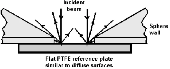
Figure 3. 5 Hemispheric reflectance

This device (see Fig. 3.5) consists of a cavity covered with a highly reflective diffusion material, with two small openings, or ports, one to allow the incident beam to enter, the other to allow to observe the radiation in this sphere. Of course the expression that provides the hemispherical reflectance, as discussed in detail later, will be calculated from (3.1) integrated over a solid angle of 2π.

As for the spherical reflectance it is, in principle, measured by an opaque sphere covered by the sample placed at the centre of the integrating sphere. One side of the sample is illuminated by a collimated beam of light, the radiation is diffused in all directions and is measured by a detector that doesn’t see the target directly.

3.1.1 Hemispheric Reflectance

The importance of the hemispherical reflectance is mainly due to two reasons: The quantity that is directly measured by many commercial spectrophotometers;

It is one of the properties of a material that determine radiative equilibrium temperature (see section 3.1.4.).

The incident energy per unit area is Jμ0. The energy of the outgoing for a unit of solid angle per unit of area is: Y Jr(i,e,g).



        ₀ ₂ ₀ ₂ (, , ) 1 ) , , ( 1 e e h _J Y i e g d r i e g d r

(43)

43 Replacing to r(i,e,g) the equation (3.1) and being d_e sineded , it’s possible to obtain the equation for the hemispheric reflectance:



 



        eded H H g p w i r e h( ) ₄ ( ) ( 0) ( ) 1sin 2 0 2 / 0 0    

_{ }

 

Hemispherical reflectance can be expressed as a contribution of two different elements r_h r_hir_ha

with rhi isotropic hemispherical reflectance and rha anisotropic hemispherical reflectance, which can be expressed as:        d H H w r_hi ( ) ( ) 2 0 1 0 0



  





         d d g p w r_ha ( ) 1 4 2 0 1 0 0   

 

 

In this way we obtain:

) ( 1 H 0 rhi                   0 0 2 0 0 1 0 1 ln 2 1 2      b w r_ha So

 

_      _ _     0 0 2 0 0 1 0 0 1 ln 2 1 2 1 ) (       H w b i r_h

Developing in Taylor series:

0 0 0 0 2 0 2 1 2 1 ln              

Replacing H() from (2.2) we have:

0 0 1 0 41 2 1 1 ) (          b w i r_h

Under appropriate simplifying assumptions we can define the reflectance r0, called diffusive (Hapke, 1993), the ratio:

(44)

44 in em P P r ₀

Where Pin is the total energy incident on the material per unit area



  /2 0 0 0cos 2 sin       d I I P_in

where I0 is the intensity of incident ray in the normal way.

Pem is the total energy spread in all directions emerging per unit area:

0 0 0 1 2 / 0 1 ₁ 1 ) 0 ( sin 2 cos ) 0 ( d I I I r I P_em                



I1(0) is the reflection in the normal direction Then:      1 1 0 r

Finally we find, inverting the (2.3) that

0 0 1 1 r r     and ₂ 0 0 ) 1 ( 4 r r w   .

As a result it can be established that by introducing the parameters K 'and S', respectively the volumetric absorption coefficient and the coefficient of volumetric scattering Kubelka-Munk, the equation of Kubelka-Munk. The extinction coefficient is to be defined as (K '+ S'). Through these parameters it’s possible to redefine the single volume scattering albedo as

' 2 ' ' 2 ' S K S w   Hereupon ' 1 ' w 