Set theory for knowledge representation

(1)

UNIVERSITY OF CATANIA

Department of Mathematics and Computer Science

SET THEORY FOR

KNOWLEDGE REPRESENTATION

Cristiano Longo

A dissertation submitted in partial fulfilment of the requirements for the degree of Doctor of Philosophy

Tesi presentata per il conseguimento del titolo di “Dottore di Ricerca in Informatica” (XXIV ciclo)

Coordinatore e Tutor

(2)

Chapter 1 Introduction

During the last century Set Theory played a central role in the development of modern mathematics, as it provided a single foundation for the diverse areas of this discipline. For example, the intuitive content of geometry, arith-metic, and analysis has been re-expressed in set-theoretic terms in entirely precise formal fashion.

The decision problem in set theory has been intensively investigated in the last decades, thus giving rise to the novel research field of Computable Set Theory, devoted to study the decision problem for fragments of set theory (see [11, 15] for a thorough account of the state-of-the-art until 2001).

The motivation which initially animated this research stream was the de-sign and implementation of an interactive proof checker, envisaged by Jackob T. Schwartz1 _{in [41], supposed to accept sequences of logical formulae, such}

that any formula in the sequence follows logically from earlier formulae. In addition, such a system should include also an inferential core, based on the very expressive formalism of set theory, to handle elementary inferential steps, in order to keep at a reasonable level the mass of details in proofs.

Over the years, decision procedures or proofs of undecidability have been provided for several quantified and unquantified fragments of set theory. It is to be noticed, however, that several decision procedures found so far are not practical at all and their interest is limited to the foundational pur-pose of identifying the boundary between the decidable and the undecidable in set theory, while the most efficient decision procedures devised in this context have been implemented in the inferential core of the proof verifier ÆtnaNova/Referee, described in [16, 33, 42].

The first unquantified sublanguage of set theory that has been proved decidable is Multi-Level Syllogistic (in short MLS, cf. [19]). MLS involves the set predicates ∈, ⊆, =, the Boolean set operators ∪, ∩, \, and the connectives of propositional logic (see Section 2.2 for the precise definitions of MLS syntax and semantics). Subsequently, several extensions of MLS with various combinations of operators (such as singleton, powerset, unionset,

(5)

etc.) and predicates (on finiteness, transitivity, etc.) have been proved to have a solvable satisfiability problem.

Also, some extensions of MLS with various map2 _{constructs have been}

shown to be decidable. In [19] a two-sorted extension of MLS is presented, where the two sorts indicate respectively set variables and map variables, and which contains the domain, range, direct and inverse image operators on maps. Additionally, this language allows assertions meaning that a map term is single-valued (i.e. it is a function) or bijective. However, the decision procedure proposed there had a double exponential time complexity. We mention also a one-sorted version of the language considered in [19], further extended with map evaluation (cf. [17]). In this case, since there is no distinction between set and map variables, maps can be combined with the Boolean set operators as well. However, the language in [17] does not allow a predicate is map(x), asserting that x is a collection of pairs. Therefore, for instance, a predicate of type Inverse(f, g) expresses only that g is an inverse of f , up to non-pair elements, so that Inverse(f, g) and Inverse(f, g′) do not imply that g = g′, but only that g and g′ contain the same pairs (namely the inverse of the pairs contained in f ). Despite the peculiarity of such semantics, the decision procedure given in [17] has a nondeterministic exponential time complexity.

Concerning quantified fragments, of particular interest to us is the re-stricted quantified fragment of set theory ∀0, viewed in Section 2.3, which

has been proved to have a decidable satisfiability problem in [6]. We re-call that ∀0-formulae are propositional combinations of restricted quantified

prenex formulae (∀y1 ∈ z1) · · · (∀yn ∈ zn)p, where p is a Boolean

combina-tion of atoms of the forms x ∈ y, x = y, and no zj is a yi(i.e., nesting among

quantified variables is not allowed). The same paper considered also the ex-tension with another sort of variables representing single-valued maps, the map domain operator, and terms of the form f (t) (representing the value of the map f on a function-free term t). However, neither one-to-many, nor many-to-one, nor many-to-many relationships can be represented in this lan-guage. We observe that the ∀0-fragment is very close to the undecidability

boundary, as shown in [37]. In fact, if nesting among quantified variables in prenex formulae of type (∀y1 ∈ z1) · · · (∀yn ∈ zn)p are allowed and a

predi-cate stating that a set is an unordered pair is also admitted, then it turns out that the satisfiability for the resulting collection of formulae is undecidable. In this thesis we study the decision problem for three novel quantified fragments of set theory, which we denote as the ∀π-family of languages. The expressive power of languages of this family is measured in terms of set-theoretical constructs they allow to express. In addition, these languages can be profitably employed in knowledge representation, since they allow to express a large amount of description logic constructs (cf. Section 3).

(6)

1.1 Knowledge Representation

As mentioned before, set theory allows to define in a elegant and precise way all common mathematical notions. Furthermore (and consequently) it can be used to represent knowledge about several domains in a simple and formal fashion. For this reason, we investigated the application of Computable Set Theory to knowledge representation, the field of Artificial Intelligence which deals with formalisms that are both epistemiologically and computationally adequate to represent knowledge about different domains.

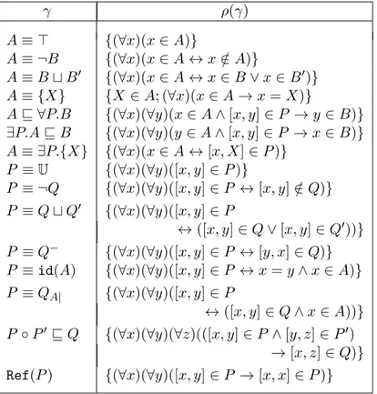
Description Logics (see [2] for an introduction) are a family of logic based formalisms widely used in knowledge representation. Several results and de-cision procedures devised in this context have been profitably employed in the area of the Semantic Web (cf. [5]). For example, the description logic SROIQ, described in [24], underpins the semantic web language OWL 2. Description Logics are logic-based formalisms that allow to represent knowl-edge about a domain of interest in terms of concepts, which denote sets of elements, roles, which represent relations between elements, and individuals, that denote domain elements. Each description logic is mainly characterized by a set of constructors, which allow to form complex terms starting from concept, role and individual names. Finally, a description logic knowledge base is a finite set of constraints on the domain structure. The most com-mon description logic constructs are listed in Tables 3.1, 3.2, and 3.3. The description logic framework will be discussed in details in Chapter 3.

1.1.1 SWRL Rules

Other approaches to knowledge representation are those related with Horn-Style rules. SWRL rules are a simple form of Horn-style rules which were proposed in [26] with the aim of increasing the expressive power of descrip-tion logics. It must be noticed that extending descripdescrip-tion logics with SWRL rules in general leads to undecidability. In [32] this issue has been overcome by restricting the applicability of rules to a finite set of named individuals. Another approach, studied in [29], consists in restricting the set of allowed rules to those which can be internalized, i.e. which can be converted into description logic statements.

1.2 Metamodeling

Description logics strictly separate the conceptual layer, which defines classes and properties, from the data layer, which contains domain objects. As a consequence, such framework does not allow metamodeling, namely the ability to define meta-concepts (i.e., concepts containing other concepts and roles) or meta-roles (i.e., relationships among concepts or among roles). We clarify the notion of metamodeling by way of an example originally presented

(7)

in [46]. Let us consider the “IUCN Red List3 _{of endangered species,” and}

let Eagle be a species in this list. Furthermore, let Harry be an eagle. The membership relations among the three items RedList , Harry, and Eagle cannot be accurately modeled in description logics, since Eagle should be simultaneously a concept, as it contains Harry as member, and an individual, since it is a member of RedList . Furthermore, there is no (intuitive) way to arrange a description logic knowledge base in such a way that an automated agent can infer that Harry cannot be hunted from the fact that it is a member of RedList .

The lack of metamodeling features is sometimes perceived as a crucial limitation of the description logics framework. For example, metamodeling was one of the original goals of the Semantic Web Language, and the earlier version of this language, called OWL Full, was expressive enough to include features of this sort. However, it turned out that this language is undecid-able, as proved in [31], where a decidable restriction of OWL Full relative to two alternative semantics, the contextual and the HiLog semantics, has been proposed. Specifically, in the contextual semantics (also known as pun-ning), identifiers are interpreted as individuals or as concepts, depending on the context, but the individual and the corresponding concept are treated as entirely independent, so that some of the expected conclusions can not be drawn (for example from Eagle(Harry), ¬Aquila(Harry) it does not descend that the individuals associated to Eagle and Aquila must be distinct). The HiLog semantics is not affected by this issue. However, it has some conse-quences which may be considered counterintuitive, as they contrast with the Zermelo-Fraenkel axiomatization of set theory (which instead underpins the family of ∀π languages). For example, a knowledge base {A(B), B(A)} is consistent under this semantics, in contrast with the regularity axiom; also, we may have two distinct domain items whose concept and role extensions coincide, thus contradicting the extensionality axiom.

Another strategy to enforce Semantic Web with metamodeling capabil-ities consists in adding on top of a domain knowledge base a separate one, which contains meta-knowledge about concepts and relationships among them. Then the two knowledge bases are kept in sync by some additional external mechanisms. This is the approach followed, for example, in [45] and, with slight modifications, in [21]. However, in our opinion, it does not apply very well to knowledge domains with more than two levels of nesting, which are not strictly stratified (i.e., when an item can be simultaneously member of two or more items placed at different levels). This issue also affects the Fixed Layered Metamodeling Architecture, studied in [35, 34].

3

(8)

1.3 The ∀

π

Family

In this thesis we present a collection of decidable quantified fragments of set theory, called the ∀π _{family (see Chapter 4), which allow the explicit}

manipulation of ordered pairs, and which can be profitably employed as knowledge representation languages.

We present a decision procedure for each language of this family, and prove that all of these procedures are optimal (in the sense that they run in nondeterministic polynomial-time) when restricted to formulae with quanti-fier nesting bounded by a constant. A considerable amount of set-theoretic constructs can be expressed by the languages in this family, also in the re-stricted case. In particular map-related constructs like map inverse, Boolean operator among maps, map transitivity, and so on, are expressible. In addi-tion, the quantified nature of these languages and the pair-related constructs they provide allow to map numerous description logic constructs into them in a very natural way, showing that these languages can effectively serve to knowledge representation.

A restricted set of SWRL rules, namely those which do not contains data literals, can be easily embedded in all the languages of the ∀π _{family without}

disrupting decidability.

Finally, as language terms are interpreted as sets in the von Neumann standard cumulative hierarchy V, described later, the semantics of our lan-guages is multi-level, so that these lanlan-guages can embody metamodeling in a very natural way.

1.4 Contributions

The main contributions of this thesis are in the field of Computable Set The-ory. The decidability of the languages in the ∀π family is helpful in defining the boundary between decidable and undecidable quantified fragments of set theory.

In addition, we consider the proof of the NP-completeness of the satisfi-ability problem for formulae in the unquantified language MLSS×_2,m, carried out in Section 5.1 by means of a straightforward reduction to the satisfiability problem for formulae in a language of the ∀π family, a significant advance-ment in the study of set-theoretical languages with map-related operators, in particular languages which allows the Cartesian product. Concerning this, we recall that extending MLS with Cartesian product and cardinality comparison leads to undecidability.

Comparison of Computable Set Theory with the description logics frame-work brought some interesting results in both these areas. Regarding Com-putable Set Theory, in Section 5.1.3 the ExpTime-hardness of the unsat-isfiability problem for every MLS extension which contains the map image operator is derived from an analogous result for the description logic ALC.

(9)

On the description logic side, the result obtained in Section 5.2 shows that imposing some restrictions on the usage of existential quantifier con-structs allows one to identify a very expressive description logic, which we denote as DL⟨∀π_{⟩, for which the consistency problem is NP-complete. In}

addition, it can be equipped with metamodeling-features in such a way that the consistency problem remains NP-complete. Finally, both DL⟨∀π_{⟩ and}

its metamodeling-enabled version remain decidables also if extended with SWRL rules.

1.5 Thesis Organization

The rest of this thesis is organized as follows. Chapters 2 and 3 provide a short introduction to Computable Set Theory and description logics, re-spectively, where their basic notions and some languages of our interest are briefly reviewed.

Chapter 4 introduces the three quantified fragments of set theory ∀π₀, ∀π

0,2, and ∀π∆, which together constitute the ∀π family. In the same chapter,

these language are proved to have a decidable decision problem, which is NP-complete when restricting to formulae whose quantifier prefix lengths are bounded by a constant.

In Chapter 5 we study the expressive power of ∀π _{languages. To this}

purpose, we present the unquantified fragment of set theory MLSS×_2,m and the description logic DL⟨∀π_{⟩, which are both expressible in a restriction of}

∀π

0,2characterized by an NP-complete decision problem. In the same chapter

we show that extending MLSS×_2,m (and thus also ∀π

0,2) with the map image

operator, or with the map domain operator, would trigger the ExpTime-hardness of the decision problem. Finally, we prove that DL⟨∀π⟩ can be extended with SWRL rules and metamodeling features, but still remaining decidable.

Finally, in Chapter 6 we draw our conclusions giving also some hints to future works.

(10)

Chapter 2 Computable Set Theory

In this chapter we give a brief overview of Computable Set Theory. In particular, we will review MLS, which has been the first sublanguage of set theory to be studied in this context. Then, we will focus our attention on MLS extensions which involve constructs related to multi-valued maps. Finally, the quantified language ∀0 will be discussed. All of the languages

mentioned in this chapter have been proved to be decidable. However, no decision procedure is reported here, rather the decidability of some of these fragments will be proved in Chapter 4, by way of reductions to languages in the ∀π _{family, presented there.}

To begin with, we define a general setup for set-theoretical languages by introducing some useful notations and definitions.

2.1 Preliminaries

Computable Set Theory focuses on decidable fragments of set theory. We will refer to the Zermelo-Fraenkel axiomatization of set theory, and we will restrict out attention to pure sets, i.e. sets whose members are sets recur-sively founded by the empty set ∅. We recall that the von Neumann standard cumulative hierarchy of sets V is the class containing all the pure sets. This hierarchy is defined by

V0 = ∅

Vγ+1 = P(Vγ) , for each ordinal γ

Vλ = _µ<λVµ, for each limit ordinal λ

V = 

γ∈OnVγ,

where P(·) is the powerset operator and On denotes the class of all ordinals. It can be proved that the membership relation is well-founded in V and, therefore, no membership cycle can occur in V.

We denote with rank(u) the least ordinal γ such that u ⊆ Vγ (i.e., u ∈

Vγ+1), for every set u in V.

The basic constituents of the languages studied in the context of Com-putable Set Theory are variables. In the rest of this thesis, we will denote

(11)

with Vars = {x, y, z, . . .} the denumerable infinite set of variables. In ad-dition, some fragments which allow map-related or pair-related constructs will make also use of another sort of variables, map variables, which are intended to denote multi-valued maps; their collection will be denoted by Varsm = {f, g, h, . . .}. For the sake of conciseness, we will assume that

Varsm is just a sub-sort of Vars (i.e. Varsm ⊆ Vars), and we will denote

with Varss the remaining variables (i.e. Varss = Vars \ Varsm), which we

call set variables.

Given any set theoretic formula ϕ, we will denote with ϕx

y the formula

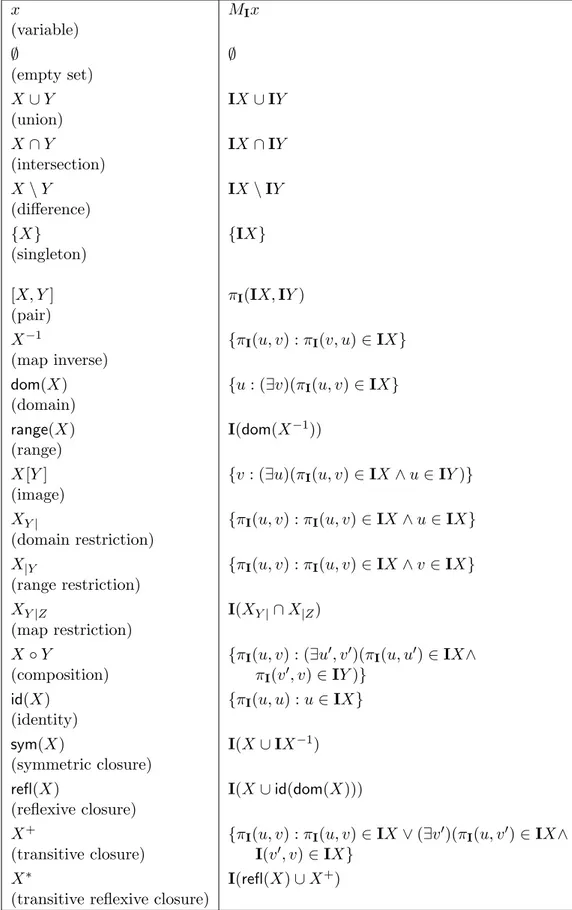
obtained by replacing each occurrence of x in ϕ with y, with x, y ∈ Vars. Variables can be combined together to form complex terms by means of the usual set theoretic operators (see Table 2.1, left column). In particular, any term of the form [X, Y ], where X, Y are set theoretical terms, represent the ordered pair of X and Y .

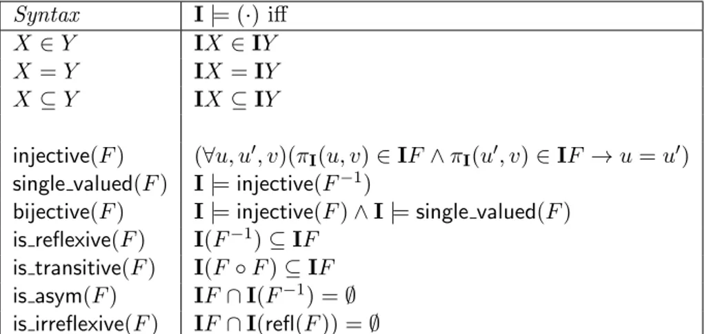
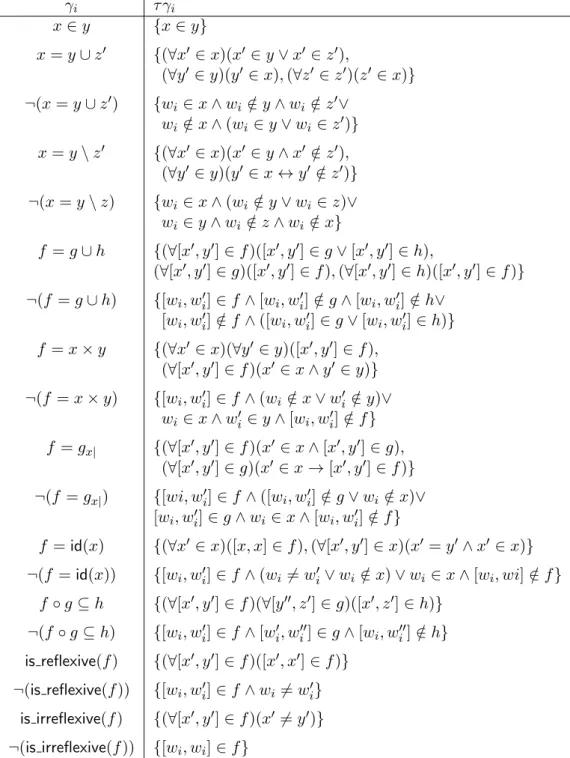
Finally, formulae of our languages are built from the atomic formulae, described in Table 2.2, using the connectives of propositional logic and, in quantified fragments, also the quantifiers ∀ and ∃.

In the next sections we provide a background semantics, which will be specialized for each fragment of set theory presented in the following. To this purpose it is useful to recall first the notion of ordered pairs.

2.1.1 Ordered Pairs

We remark that multi-valued maps are just sets consisting only of ordered pairs. Thus, for our purposes, it is useful to recall some notions concerning ordered pairs in set theory.

Ordered pairs are represented in set theory by means of pairing functions. In order to provide the precise definition of such kind of operations, we need first to recall that, given an injective binary operation over sets π, and two sets u, v, the Cartesian product of u and v with respect to π, denoted by u × v, can be defined as follows:

u × v = {π(u′, v′) : u′ ∈ u ∧ v′ ∈ v}.

Definition 1. Let π be a binary operation over sets in V. π is said to be a pairing function if and only if the following conditions hold:

(P1) π(u, v) = π(u′, v′) ⇐⇒ u = u′ ∧ v = v′_{, and}

(P2) u × v is a set in V for any u, v, u′, v′ ∈ V.

Let π be a pairing function, and let u be a set in the von Neumann hierarchy. We denote with π(u) the set consisting of the pair members of u, with respect to the pairing function π. More formally

π(u) = {π(v, v′) : π(v, v′) ∈ u}.

(12)

Syntax I(·) x MIx (variable) ∅ ∅ (empty set) X ∪ Y IX ∪ IY (union) X ∩ Y IX ∩ IY (intersection) X \ Y IX \ IY (difference) {X} {IX} (singleton) [X, Y ] πI(IX, IY ) (pair) X−1 {π_I(u, v) : πI(v, u) ∈ IX} (map inverse)

dom(X) {u : (∃v)(π_I(u, v) ∈ IX} (domain)

range(X) I(dom(X−1)) (range)

X[Y ] {v : (∃u)(π_I(u, v) ∈ IX ∧ u ∈ IY )} (image)

XY | {πI(u, v) : πI(u, v) ∈ IX ∧ u ∈ IX}

(domain restriction)

X|Y {πI(u, v) : πI(u, v) ∈ IX ∧ v ∈ IX}

(range restriction)

X_{Y |Z} I(X_{Y |}∩ X_|Z) (map restriction)

X ◦ Y {π_I(u, v) : (∃u′, v′)(πI(u, u′) ∈ IX∧

(composition) πI(v′, v) ∈ IY )}

id(X) {π_I(u, u) : u ∈ IX} (identity)

sym(X) I(X ∪ IX−1) (symmetric closure)

refl(X) I(X ∪ id(dom(X))) (reflexive closure)

X+ {π_I(u, v) : πI(u, v) ∈ IX ∨ (∃v′)(πI(u, v′) ∈ IX∧

(transitive closure) I(v′, v) ∈ IX} X∗ I(refl(X) ∪ X+) (transitive reflexive closure)

(13)

Syntax I |= (·) iff X ∈ Y IX ∈ IY X = Y IX = IY X ⊆ Y IX ⊆ IY

injective(F ) (∀u, u′, v)(πI(u, v) ∈ IF ∧ πI(u′, v) ∈ IF → u = u′)

single valued(F ) I |= injective(F−1)

bijective(F ) I |= injective(F ) ∧ I |= single valued(F ) is reflexive(F ) I(F−1) ⊆ IF

is transitive(F ) I(F ◦ F ) ⊆ IF is asym(F ) IF ∩ I(F−1) = ∅ is irreflexive(F ) IF ∩ I(refl(F )) = ∅

Table 2.2: Set-theoretic atomic formulae

2.1.2 Background Semantics

Now we provide some notions and definitions that will be used in the se-mantics definitions of the fragments presented later.

To begin with, we will refer to mappings from variables to sets in V as assignments. Let W be a finite subset of Vars, and let M, M′be assignments. Then M′ is said to be a W -variant of M if M′x = M x for all x ∈ Vars \ W (i.e. M and M′ coincides except for the variables in W ).

A set-theoretic interpretation is a pair I = (MI, πI), where MI is an

assignment, and πI is a pairing function. We characterize this kind of

inter-pretation as set-theoretic in order to distinguish them from the descriptive interpretations of description logic, which will be defined in Chapter 3. How-ever, we will omit to indicate the interpretation type when it will be clear from the context.

The notion of W -variant is extended to interpretations as expected. Thus, let W be a finite subset of Vars, and let I, I′ be two interpretations. I′ is said to be a W -variant of I if and only if

• πI′ = π_I, and

• MI′ is a W -variant of M_I.

An interpretation I associates sets in V to terms as indicated in Table 2.1, right column. Furthermore, interpretations evaluate set-theoretic formulae to a truth value true or false. We say that an interpretation I is a model for a formula ϕ if I evaluates ϕ to true. In this case, we write I |= ϕ. Otherwise, if I evaluates a formula ϕ to false, we write I ̸|= ϕ.

A formula is said to be satisfiable if it admits a model, otherwise it is said to be unsatisfiable. Thus, the satisfiability problem (in short s.p.) consists in determining whether a formula is satisfiable or not.

Evaluation of formulae for each of the languages described in this chap-ter will be defined in a precise way when the languages will be presented.

(14)

However, evaluation of atomic formulae is carried out as indicated in Table 2.2, right column.

We conclude this section with some definitions concerning interpreta-tions. Let W be any collection of variables. An interpretation I is said to be pair-free with respect to W if

πI(MIx) = ∅

for each x ∈ W , that is, I associates to variables in W only sets which do not contain any pair. An interpretation is said to be just pair-free if it is pair-free with respect to the whole set of variables Vars.

Finally, an interpretation I is said to be pair-safe if it associates just sets of ordered pairs (or the empty set) to map variables. In other words, I is pair-safe if and only if

MIf = πI(MIf )

for each f ∈ Varsm.

In the next section we will examine some unquantified fragments of set theory, starting from the basic languages MLS and MLSS, and then reviewing some MLSS extensions with map constructs.

2.2 Multi-Level Syllogistic

As mentioned before, Multi-Level Syllogistic (in short MLS) has been the first unquantified language studied in the context of Computable Set Theory. MLS is a fragment of set theory which contains:

1. the denumerable infinity of variables Vars; 2. the set-theoretical operators ∪, ∩, \;

3. the relators ∈, =;

4. the Boolean connectives of propositional logic.

The set of the terms allowed in this language, which we call the set of MLS-terms, is defined by the following syntax rule:

X, Y −→ x | X ∪ Y | X ∩ Y | X \ Y

where x is a variable, and X, Y are MLS-terms. Atomic MLS-formulae are atomic formulae of the types

X ∈ Y, X = Y

where X and Y are MLS-terms. Finally, MLS-formulae are Boolean combi-nations of atomic MLS-formulae by means of the connectives of propositional logic. Then, evaluation of MLS-formulae by interpretations is carried out as

(15)

usual in propositional logic, assuming that atomic formulae are evaluated as indicated in Table 2.2.

The language MLSS (Multi-Level Syllogistic with Singleton) is obtained by extending MLS with the singleton operator {X}. In more details, the set of MLSS -terms is defined by

X, Y −→ x | X ∪ Y | X ∩ Y | X \ Y | {X}

where x is a variable, and X, Y are MLSS-terms. Again, MLSS -formulae are Boolean combinations of atomic formulae, and evaluation of MLSS-formulae follows the standard rules.

In the next section we review some extensions involving map constructs. It must be noticed that the satisfiability problem for formulae of the lan-guages presented in the next section is ExpTime-hard, as reported in The-orem 2.

2.2.1 Multi-Level Syllogistic with Maps

The first MLS extension involving maps we examine is that studied in [17], which we denote by MLSm, where the subscript indicates the presence of

map related operators. MLSm -terms are formed according to the following

syntax rule:

X, Y, Z −→ x | X ∪ Y | X ∩ Y | X \ Y | dom(X) | range(X) | X[Y ] | X−1 | XY || X|Y | XY |Z

where x ∈ Vars, and X, Y, Z are MLSm-terms. Atomic MLSm -formulae are

of the following types:

[X, Y ] ∈ Z, X ∈ Y, X = Y,

injective(X), single valued(X), bijective(X),

where X, Y, Z are MLSm-terms. Finally, MLSm-formulae are Boolean

com-binations of atomic MLSS-formulae.

Another approach to extend MLS with map constructs is the one followed in [19], where a two-sorted language which contains map constructs was proved to be decidable. We denote this language as MLSm,2, where the

subscript “2” indicates that it contains two sort of variables. MLSm,2 is a fragment of set theory which contains:

1. the denumerable infinity of set variables Varss;

2. the denumerable infinity of map variables Varsm;

3. the predicate symbols single valued, bijective;

4. the operator symbols ∪, ∩, \, dom, range, f−1 (map inverse), f [x] (image);

(16)

5. the relators ∈, =;

6. the Boolean connectives of propositional logic.

MLSm,2 -terms are defined according to the following syntax rules:

X, Y −→ x | X ∪ Y | X ∩ Y | X \ Y | f | dom(F ) | range(F ) | f [X] | f−1[X]

where x and f stay respectively for set and map variables, and X, Y for MLSm,2-terms. Atomic MLSm,2 -formulae are set-theoretic expressions of

the types X ∈ Y , X = Y , single valued(f ), and bijective(f ), where X, Y are MLSm,2-terms, and f is a map variable. We remark that the decidability

of the s.p. for MLSm,2-formulae was proved in [19] with presenting a double

exponential-time decision procedure.

Up to this point, we illustrated just unquantified languages devised in the context of Computable Set Theory. In the next section we review a quantified fragment, called ∀0.

2.3 The Language ∀

₀

In this section we discuss the quantified fragment of set theory ∀0, studied

in [6]. We recall that decision procedures for this language can be found in [6, 8]. In particular, the decision procedure presented in [8] is optimal, since it runs in nondeterministic-polynomial time. However, we do not report this decision procedure, as we provide instead a reduction of the satisfiability problem for formulae of this language to one of the languages in the ∀π -family (which will be proved to be decidable later), that will be introduced and discussed in Chapter 4.

The language ∀0 contains:

• the variables in Vars; • the set relators ∈, =;

• the universal quantifiers ∀, ∃; • parentheses;

• the logical connectives ¬, ∧, ∨, →, ↔.

The set of the ∀0 -formulae is defined as follows. Atomic ∀0 -formulae

are atomic formulae of the types x ∈ y, x = y (pairs are not allowed in this language), with x, y ∈ Vars. Quantifier-free ∀0 -formulae are Boolean

com-binations of atomic ∀0-formulae by means of the propositional connectives.

Finally, ∀0-formulae1 are quantified formulae of the form

Q1Q2. . . Qnψ

(17)

where

• ψ is a quantifier-free ∀0-formula;

• n is a non-negative integer;

• for 1 ≤ i ≤ n, either every Qi is a restricted quantifier of the form

(∀xi ∈ yi), or every Qi is of the form (∃xi ∈ yi) (we will refer to xi as

quantified variables and to yi as domain variables, for 1 ≤ i ≤ n);

• nesting among quantified variables is not allowed (more precisely, no yj is a xi, for all 1 ≤ i, j ≤ n).

It must be noticed that, in the previous definition, if we restrict to the case n = 0 we get the class of quantifier-free ∀0-formulae. In other words,

all the quantifier-free ∀0-formulae are ∀0-formulae.

Given any ∀0-formula ϕ, we denote with Vars(ϕ) the set of the free

vari-ables in ϕ, i.e. all the varivari-ables which occur not bounded by any quantifier in ϕ.

The ∀0 semantics extends the background semantics introduced above to

cope with universal quantifiers. Then, evaluation of quantifier-free formulae is carried out as usual, while, given any interpretation I, I evaluates to true a quantified ∀0-formulae of the form (∀x ∈ y)χ, with x, y ∈ Vars, if and

(18)

Chapter 3 Description Logics

Description Logics are a well-established and well-studied framework for knowledge representation (see [2] for a quite complete introduction to this family of languages). They are logic-based languages which allow to provide a high-level description of the world in a formal and precise way. More in details, knowledge about a domain of interest is described in terms of con-cepts, which denote sets of elements, roles, which represent relations between elements, and individuals, that denote domain elements. Then, a description logic knowledge base is a finite description of the world, expressed by means of a finite set of constraints involving concepts, roles, and individuals.

Over the years, description logics have been employed in several applica-tion domains such as natural language processing, configuraapplica-tion, data bases and medicine. Most notably, they have been adopted in the context of Se-mantic Web (cf. [5]) to provide solid seSe-mantical foundations to the SeSe-mantic Web Language OWL1 _{(see for example [25]).}

In contrast with other earlier knowledge representation approaches such as, for example, Semantic Networks (cf. [40]), description logics are equipped with a well-defined syntax, and a formal, unambiguous semantics. In ad-dition, the description logic framework provides effective mechanisms for reasoning, which allow to extract implicit knowledge from the knowledge explicitly stated in a knowledge base. The main reasoning tasks identified in this context are:

• concept satisfiability, which allows to determine whether a complex concept can be interpreted (description logic interpretation will be de-fined in a precise way later in this chapter) by a non-empty set of domain elements;

• concepts subsumption, i.e. testing if a concept subsumes another con-cept;

• instance checking, which allows to determine whether an individual belongs to a given concept;

(19)

• instance retrieval, which consists in retrieving all the individuals be-longing to a given concept;

• entailment, i.e. testing if, given two knowledge bases K and K′_{, the}

facts stated in K′ are consequences of those contained in K.

However, the main reasoning task for description logics is consistency check, which consists in determining whether the information contained in a knowledge base is self-contradictory or not, since, except for some weaker description logics, all the other reasoning tasks can be reduced to it. For this reason, when we will use the term “reasoning” without being more specific, we will refer to consistency check. Consistency check, along with the other reasoning tasks, will be defined formally in Section 3.1.

In the last decades sound and complete algorithms were devised for a considerable amount of description logics, and optimized versions of these algorithms have been implemented in several reasoning engines like FaCT, Race, and DLP (cf. [23, 22, 39]).

The trade-off between the expressive power (in terms of allowed con-structs) and the computational complexity of reasoning is actually one of the major research topics in description logics. In fact, while the reasoning for the basic description logic AL is ExpTime-hard (cf. [2, Theorem 3.27, page 132]), and this may be prohibitive for practical applications, a lower computational complexity can be achieved by choosing appropriately the set of allowed constructs (see [7] and [1] for some examples of description logics with polynomial-time reasoning).

This chapter aims to provide a brief overview of the description logic framework, by reviewing some of these logics of our interest. We introduce this framework by describing the basic description logic ALC, and then we discuss some of its expressive extensions. Finally, we will examine an extension of this framework based on Horn-like rules, namely SWRL rules, proposed in [26]. As we did in Chapter 2, we begin with providing the general notions and definitions of this framework.

3.1 Preliminaries

As mentioned before, a description logic knowledge base describes a knowl-edge domain in terms of concepts, roles, and individuals. The building blocks of description logics are

• a countably infinite collection of concept names Nc_{= {A, B, . . .},}

• a countably infinite collection of role names Nr _{= {P, Q, . . .}, and}

• a countably infinite collection of individual names Ni _{= {a, b, . . .}.}

Each description logic is mainly characterized by a set of concept and role constructors, which, starting from the basic names in Nc, Nr, and Ni,

(20)

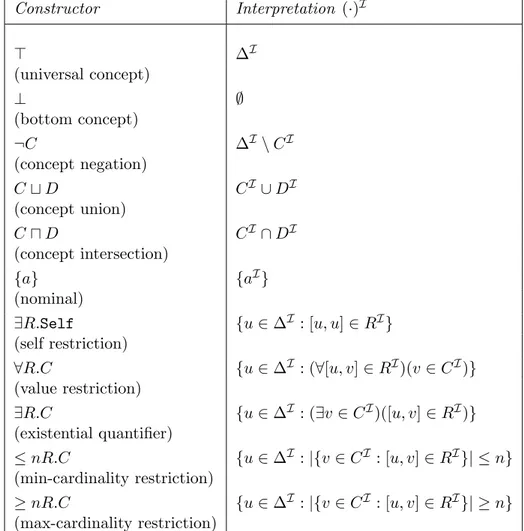
Constructor Interpretation (·)I ⊤ ∆I (universal concept) ⊥ ∅ (bottom concept) ¬C ∆I\ CI (concept negation) C ⊔ D CI∪ DI (concept union) C ⊓ D CI∩ DI (concept intersection) {a} {aI} (nominal) ∃R.Self {u ∈ ∆I : [u, u] ∈ RI} (self restriction) ∀R.C {u ∈ ∆I : (∀[u, v] ∈ RI)(v ∈ CI)} (value restriction) ∃R.C {u ∈ ∆I : (∃v ∈ CI)([u, v] ∈ RI)} (existential quantifier) ≤ nR.C {u ∈ ∆I : |{v ∈ CI : [u, v] ∈ RI}| ≤ n} (min-cardinality restriction) ≥ nR.C {u ∈ ∆I : |{v ∈ CI : [u, v] ∈ RI}| ≥ n} (max-cardinality restriction)

Table 3.1: Description logic concept constructors

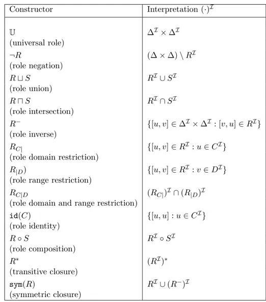
allow to form complex concepts and roles. Thus, description logic terms are divided into concept and role terms: concept terms are concept names and complex concepts constructed by means of the concept constructors; analogously, role terms are role names and complex roles constructed by means of role constructors. Some of the most common constructors used in description logics are listed in Tables 3.1 and 3.2, where C, D are concepts, R, S are roles, and a is an individual name.

In general, we will use the terms “concepts” and “roles” to indicate concept and role terms, respectively.

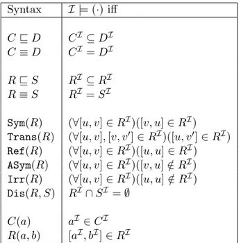
Description logics are also characterized by the types of constraints they allow to be specified in knowledge bases. These constraints (see Table 3.3) can be of three different types: concepts inclusions of the form C ⊑ D, role inclusions R ⊑ S, and assertions like C(a), R(a, b), concerning the mem-bership of individuals or individual pairs to concepts and roles, respectively. In addition, some expressive description logic allow also constraints stating properties of roles, for example Trans(R), which expresses the fact that the

(21)

Constructor Interpretation (·)I U ∆I× ∆I (universal role) ¬R (∆ × ∆) \ RI (role negation) R ⊔ S RI∪ SI (role union) R ⊓ S RI∩ SI (role intersection) R− {[u, v] ∈ ∆I× ∆I : [v, u] ∈ RI} (role inverse) RC| {[u, v] ∈ RI : u ∈ CI}

(role domain restriction)

R|D) {[u, v] ∈ RI : v ∈ DI}

(role range restriction)

RC|D (RC|)I ∩ (R|D)I

(role domain and range restriction)

id(C) {[u, u] : u ∈ CI} (role identity) R ◦ S RI◦ SI (role composition) R∗ (RI)∗ (transitive closure) sym(R) RI∪ (R−)I (symmetric closure)

(22)

Syntax I |= (·) iff C ⊑ D CI ⊆ DI C ≡ D CI = DI R ⊑ S RI ⊆ RI R ≡ S RI = SI Sym(R) (∀[u, v] ∈ RI)([v, u] ∈ RI) Trans(R) (∀[u, v], [v, v′] ∈ RI)([u, v′] ∈ RI) Ref(R) (∀[u, v] ∈ RI)([u, u] ∈ RI) ASym(R) (∀[u, v] ∈ RI)([v, u] /∈ RI₎

Irr(R) (∀[u, v] ∈ RI)([u, u] /∈ RI) Dis(R, S) RI∩ SI = ∅

C(a) aI ∈ CI R(a, b) [aI, bI] ∈ RI

Table 3.3: Knowledge base constraints

role R must be a transitive relation.

Then a description logic knowledge base is a finite set of constraints of the types listed in Table 3.3, left column, where C, D are concepts, R, S are roles, and a, b are individual names.

Description logic semantics2 is given in terms of descriptive interpreta-tions. An interpretation I = (∆I, ·I) consists of a nonempty set ∆I, namely the interpretation domain, and an interpretation function ·I assigning to each concept name a subset of ∆I, to every role name a relation over ∆I, and to every individual name a domain item in ∆I. An interpretation I extends recursively to complex terms as indicated in the right column of Tables 3.1 and 3.2.

An interpretation I evaluates a description logic constraint γ to a truth value true or false. We say that an interpretation I satisfies a constraint γ, and write I |= γ, if I evaluates γ to true, otherwise we write I ̸|= γ. Evaluation of knowledge base constraints is carried out as indicated in the right column of Table 3.3.

If an interpretation I satisfies all the constraints in a knowledge base K, then I is said to be a model for K, and we write I |= K. A knowledge base is said to be consistent if it admits a model. Thus the consistency problem for description logic knowledge bases is to determine whether a knowledge base is consistent or not.

We conclude this section with the precise definitions of the other reason-ing tasks mentioned before.

2_{Here we will limit ourselves to the descriptive semantics. There are several other}

(23)

Given a concept C, we say that C is satisfiable if and only if there exists an interpretation I which associates to it a non-empty set, i.e. CI ̸= ∅. Given a knowledge base K and a concept C, C is said to be satisfiable with respect to K if K admits a model I such that CI is not empty.

Now let C, D be two concepts. We say that C subsumes D if and only if DI ⊆ CI_{, for every interpretation I. In addition, we say that C subsumes}

D with respect to the knowledge base K if and only if DI ⊆ CI _{for each}

model I of K.

Given a knowledge base K, a concept C, and an individual a, then a is said to be an instance of C with respect to K if and only if I |= C(a) for every model I of K.

The reasoning tasks called instance retrieval consists in determining which individuals are instances of the concept C with respect to the knowl-edge base K.

Finally, given two knowledge bases K and K′, we say that K entails K′ if each model of K is a model for K′ also, i.e. I |= K =⇒ I |= K′.

In the next section we recall the basic description logic ALC and then show that in ALC all the reasoning tasks we just mentioned can be reduced to knowledge base consistency.

3.2 The Description Logic ALC

ALC is one of the earlier languages devised in the context of description logics. It contains:

• a countably infinite collection of concept names Nc_{= {A, B, . . .};}

• a countably infinite collection of role names Nr _{= {P, Q, . . .};}

• the concept constructors ⊔, ⊓, ¬, ∃, ∀; • concept inclusions and equality symbols.

The collection of ALC-concepts is defined by the following syntax rule: C, D −→ A | ¬C | C ⊓ D | C ⊔ D | ∃P.C | ∀P.C

where C, D are ALC-concepts, A is a concept name in Nc_{, and P is a}

role name, while complex roles are not allowed in ALC. Finally, an ALC-knowledge base is a finite set of constraints of the following types:

C ⊑ D, C ≡ D, C(a), R(a, b)

with C, D ALC-concepts, and a, b ∈ Ni_.

The description logic ALC extends the basic description logic AL (which is an acronym for Attributive Language) by also allowing the negation of

(24)

complex concepts, while in AL concept negation is available only for concept names.

This peculiarity of ALC allows one to reduce all the reasoning tasks men-tioned above to knowledge base consistency, since complex negation allows one to express the negation of ALC-knowledge base constraints.

Plainly, a concept C is satisfiable with respect to a knowledge base K if and only if the knowledge base K ∪ {C(a)}, where a is an individual name not already occurring in K and in C, is consistent. In turn, a concept C is satisfiable (in general) if and only if it is satisfiable with respect to the empty knowledge base.

Concept subsumption can be reduced to concept (un)satisfiability, which we just proved to be reducible to knowledge base consistency, since, given any two concepts C and D, C subsumes D if and only if the concept C ⊓ ¬D is unsatisfiable.

Next, we show that the entailment of a knowledge base K′ by K can be reduced to knowledge base (un)consistency. Let us consider first the simpler case in which K′ consists of a single constraint γ. If γ is the concept inclusion C ⊑ D, for some concepts C and D, then K entails K′ = {C ⊑ D} if and only if the knowledge base K ∪ {(C ⊓ ¬D)(a)} is not consistent, for some individual name a not already occurring in K ∪ K′. Analogously, K entails {C(b)}, where C is a concept and b is an individual name, if and only if K ∪ {(¬C)(b)} is inconsistent.3

Now let K′ = {γ1, . . . γn}, for some ALC-knowledge base constraints

γ1, . . . , γn, with n ∈ N, n > 1. Then K entails K′ if and only if K entails γi,

for every 1 ≤ i ≤ n.

Finally, a knowledge base K entails that the individual a is an instance of the concept C if and only if K entails the knowledge base {C(a)}, and all the instances of C with respect to K can be retrieved by iterating the instance checking test over all the individual names occurring in K.

3.2.1 Complexity Issues

It must be noticed that the description logic ALC is not very expressive. For example, it does not contains complex roles. Despite of this, the complexity of reasoning in ALC is ExpTime-hard, and this is prohibitive for some application domains.

This complexity lower bound was proved for the weaker description logic AL in [2, Theorem 3.27, page 132], where the accessibility problem for suc-cinct representations of AND-OR graphs was reduced to concept unsatisfi-ability with respect to knowledge base consisting of concept inclusions only (see [36, 3]). Hence, the following Theorem easily follows, since AL is a sublogic of ALC.

3_{Entailment of role assertions of the form R(a, b) requires an additional constructor,}

(25)

Theorem 2. The problem of deciding whether a given ALC-concept C is un-satisfiable with respect to a finite collection of ALC-inclusions is ExpTime-hard.

We argue that this lower bound is mainly due to the presence of the quantifiers ∃ and ∀ in an unconstrained way, since their presence force any decision algorithm to invent new items when constructing a model witness-ing the consistency of a knowledge base. Intuitively speakwitness-ing, if durwitness-ing the construction process of such a model we find an item u ∈ (∃R.C)I, we may be forced to introduce a new item v ∈ CI to be placed as second item of the pair [u, v] ∈ RI. And, in ALC, this may require to introduce exponentially many new items.

This argumentation is supported by the fact that reasoning in the de-scription logic DL⟨∀π_{⟩ (studied in Section 5.2) is NP-complete despite of the}

significant amount of constructs available in this language, since the usage of quantifiers is restricted in this description logic.

In the next sections we will examine some expressive extensions of ALC.

3.3 Number Restrictions

In general, the expressive power of ALC is considered insufficient to deal with knowledge representation matters. For this reason, over the years sev-eral extensions of ALC have been studied. In this context the so called number description were devised. These are actually considered one of the most distinguishing feature of the description logic framework. Number de-scriptions, described in Table 3.1, are concept constructors which allow to impose some cardinality constraints. For example, the concept ≤ 3R.C, where R is a role and C is a concept, contains all those domain items which are connected by the role R to at most 3 domain items in the concept C. Thus, for example, the following constraint states that the role R is single-valued4

⊤ ⊑≤ 1R.⊤.

Observe that the constructors ≤ n and ≥ n are mutually expressible in those description logics which allow complex concepts negation, since ≤ nR.C ≡ ¬(≥ (n + 1)R.C) and ≥ nR.C ≡ ¬(≤ (n + 1)R.C) are valid statements.

In addition, an existential restriction ∃R.C can be expressed as ≥ 1R.C, so that the complexity upper bound provided by Theorem 2 holds also for the description logic obtained from ALC extended with number restriction, but disallowing the quantifiers.

4_{Here we used the term “single-valued”, which is typical of set-theoretical languages,}

just to avoid confusion. However, in the description logic context these kind of roles are often called functional roles.

(26)

In the next section we present the very expressive description logic SROIQ, which underpins the semantic web language OWL2.

3.4 The Description Logic SROIQ

The description logic SROIQ, devised in [24], is a very powerful descrip-tion logic which extends ALC with some advanced features concerning roles. In fact, it allows role inverses, the universal role, role inclusion constraints and role composition. However, it imposes some quite intricate syntactic restrictions. Nevertheless, the consistency problem in this language is pTime-hard, since it extends the description logic ALCQIO, whose NEx-pTime-hardness was proved in [44].

SROIQ concepts and roles are defined by means of the following syntax rules:

C, D −→ A | ¬C | C ⊓ D | C ⊔ D | ∃R.C | ∀R.C | {a} | ∃C.Self | ≤ nR.C | ≥ nR.C

R −→ P | R−

where n is a non-negative integer, A is a concept name, C and D are SROIQ-concepts, a is an individual name, P is a role name, and R is a SROIQ-role. Semantics of SROIQ concepts and roles is reported in the right column of Tables 3.1 and 3.2, respectively.

Beside the constraints allowed in ALC-knowledge bases, a SROIQ-knowledge base may contain also role inclusions, and role assertions of the following types:

Sym(R), ASym(R), Trans(R), Ref(R), Irr(R), Dis(R, S),

where R and S are SROIQ-roles. However, as mentioned before, SROIQ imposes several syntactic restrictions on knowledge base, which require some preliminary definition to be stated.

Let ≺ be a strict partial order over the set of SROIQ-roles (we recall that a relation is said to be a strict partial order if it is irreflexive and transitive). Then ≺ is said to be regular if the following holds for any pair of SROIQ-roles R and S:

S ≺ R ⇐⇒ S− ≺ R.

A role hierarchy Rh is a finite set of inclusions of the form

R1◦ . . . ◦ Rn⊑ P

where R1, . . . , Rn are SROIQ-roles not including the universal role U, and

P is a role name.

Now let ≺ be a strict partial order, and let w ⊑ P be a role inclusion, with w = R1◦. . .◦Rnfor some n > 0 and R1, . . . , RnSROIQ-roles different

from U. Then w ⊑ P is said to be ≺-regular if either one of the following conditions holds, for some role name P and for some roles S1, . . . , Sn−1:

(27)

• w = P ◦ P ; • w = P ◦ P−_;

• Ri ≺ P , for all 1 ≤ i ≤ n;

• w = P ◦ S1◦ . . . ◦ Sn−1 and Si ≺ P , for all 1 ≤ i < n;

• w = S1◦ . . . ◦ Sn−1◦ P and Si ≺ P , for all 1 ≤ i < n.

Finally, a role hierarchy Rh is said to be regular if there exists a regular

order ≺ such that each inclusion in Rh is ≺-regular.

Given a role hierarchy Rh, we denote with ⊑∗ the reflexive transitive

closure of the relation ⊑ among roles induced by Rh. Then, a SROIQ-role

R is said to be a subrole of the SROIQ-role S if R ⊑∗ S.

Role Assertions are knowledge base constraints of the following forms: Sym(R), ASym(R), Trans(R),

Ref(R), Irr(R), Dis(R, S),

where R,S are SROIQ-roles such that R, S ̸= U. Given a role hierarchy Rh, and a finite set of role assertions Ra, the set of roles that are simple in

R = Rh∪ Ra is inductively defined as follows:

• a role name is simple if it does not occur in the right-hand side of any inclusion in Rh;

• R− _{is simple if and only if so is R, for every SROIQ-role R;}

• if R occurs in the right-hand side of an inclusion in Rh, R is simple if,

for each inclusion w ⊑ R ∈ Rh, w = S for some simple role S.

A set of role assertions Ra is simple if all roles R, S appearing in role

assertions of the form Irr(R), ASym(R), or Dis(R, S), are simple in R. A SROIQ -RBox R is a set R = Rh∪ Ra, where Rh is a regular role

hierarchy, and Ra is a simple set of role assertion.

Finally, a SROIQ -knowledge base consists of • a SROIQ-RBox R = Rh∪ Ra;

• a finite set of inclusions of SROIQ-concepts, in which the terms of the forms ∃S.Self, (≤ n)R.C, and (≥ n)R.C are so that R is simple with respect to R;

• a finite set of individual assertions of the forms C(a), R(a, b), (¬R)(a, b), and a ̸= b, where a,b are individual names, C is a SROIQ-concept, and R is a SROIQ-role.

In the next section we mention another approach to augment the expres-sive power of description logics, which consists in extending description logic knowledge bases with SWRL rules.

(28)

3.5 SWRL Rules

In order to increase the expressive power of description logics, in [26] it was proposed to extend this framework with a simple form of Horn-style rules called SWRL rules. SWRL rules have the form

H → B1∧ . . . ∧ Bn

where H, B1, . . . , Bn are atoms of the forms A(x), P (x, y), x = y, x ̸= y,

with A a concept name, P a role name, and x, y either SWRL-variables or individual names.

A binding B(I) is any extension of the interpretation I which assigns a domain item to each SWRL-variable. An interpretation I satisfies a rule H → B1 ∧ . . . ∧ Bn if each binding B(I) which satisfies all the atoms

B1, . . . , Bn satisfies H also.

A description logic knowledge base K extended with a finite set of SWRL rules R is said to be consistent if and only if it admits a model which satisfies K and all the rules in R.

The great expressive power of SWRL rules leads to undecidability if used in conjunction with the description logic SROIQ. This was proved in [26] by providing a reduction to the consistency problem for SROIQ-knowledge bases5 of the Tiling Problem, a well-known undecidable problem studied in [4].

A similar undecidability result was proved in [28, Fact 4.2.2] with provid-ing a reduction of the Post Correspondence problem. The same proof shows that undecidability is not caused by the great expressive power of SROIQ, but just by the presence of existential quantifiers, in conjunction with SWRL rules.

5_{To be more precise, in [26] it was provided a reduction to the consistency problem in}

(29)

Chapter 4 The ∀

π

Family

In this chapter we introduce the ∀π family of quantified fragments of set theory, consisting of three languages which allow the explicit manipulation of ordered pairs. We will provide a decision procedure for each language in this family. Furthermore, we will prove that, when the length of quantifier prefixes is bounded by a constant, the decision procedures for the three languages run in nondeterministic-polynomial time.

4.1 The Language ∀

π₀

The language ∀π

0 is a quantified fragment of set theory which contains

• a denumerable infinity of variables Vars, defined in Section 2.1, • the binary pairing operator [·, ·],

• the monadic function ¯π(·), which yields the collection of the non-pair members of its argument,

• the relators ∈ and =,

• the Boolean connectives of propositional logic ¬, ∧, ∨, →, ↔, • parentheses, and

• the universal quantifier ∀.

A quantifier-free ∀π₀-formula is any propositional combination of atomic ∀π

0-formulae. These are expressions of the following types:

x ∈ ¯π(z), [x, y] ∈ z, x = y,

with x, y, z ∈ Vars. Intuitively, terms of the form [x, y] represent ordered pairs of sets. A prenex ∀π

0-formula is a formula of the form

(30)

with n ≥ 0, where ψ is a quantifier-free ∀π

0-formula, and the Qiare restricted

universal quantifier all of the form (∀x ∈ ¯π(y)) or all of the form (∀[x, x′] ∈ y). We will refer to x and x′ as quantified variables and to y as domain variables. A prenex ∀π

0-formula is said to be simple if no variable occurs

both as a quantified and a domain variable, i.e., roughly speaking, no x, x′ can be a y in the previous definition.

Finally, a ∀π

0-formula is any finite conjunction of simple prenex ∀π0

-formulae.

In order to provide the semantics definitions for ∀π

0, we extend

set-theoretic interpretations to terms of the form ¯π(x) as follows: I¯π(x) =DefIx \ πI(Ix)

for every interpretation I = (MI, πI), where x ∈ Vars.

According to Table 2.2, atomic ∀π

0-formulae are evaluated by a

set-theoretic interpretation I as follows:

I |= x ∈ ¯π(y) ⇐⇒ Ix ∈ I¯π(y)

I |= x = y ⇐⇒ Ix = Iy

I |= [x, y] ∈ z ⇐⇒ I[x, y] ∈ Iz. Evaluation of quantifier-free ∀π

0-formulae is carried out according to the

standard rules of propositional logic, and simple prenex ∀π

0-formulae are

evaluated as follows:

• I |= (∀x ∈ ¯π(y))ϕ iff I′ |= ϕ for every {x}-variant I′ _{of I such that}

I′x ∈ I¯π(x),

• I(∀[x, y] ∈ z)ϕ = true iff I′_{ϕ = true for every {x, y}-variant I}′ _{of I}

such that I′[x, y] ∈ Iz.

Finally, an interpretation I evaluates to true a ∀π

0-formula ϕ1∧ . . . ∧ ϕn,

where n ∈ N and ϕi are simple prenex ∀π0-formulae, for 1 ≤ i ≤ n, if and

only if it evaluates to true all the conjuncts ϕi.

In the rest of this section we present and discuss a nondeterministic de-cision procedure for ∀π₀. We begin with introducing skeletal representations, which are finite structures which represent interpretations in a concise way, in a sense that will be clarified below. We will prove that skeletal representa-tions can be used to witness the satisfiability of ∀π₀-formulae. In particular, the decision procedure presented here relies on the fact that any ∀π

0-formula

is satisfiable if and only if there exists a size-bounded skeletal representation with some peculiar characteristics.

Later, the same problem will be considered from a complexity point of view, and we will show that it is NP-complete if we restrict to formulae whose quantifier prefixes have length bounded by a constant.

(31)

4.1.1 Skeletal representations

Skeletal representations are concise representations of set-theoretic interpre-tations, in the sense that, given an interpretation I and a finite collection of variables x1, . . . , xn, one can construct a skeletal representation S which

represents in a faithful and concise manner the relationships among the sets Ixi, I[xi, xj], where 1 ≤ i, j ≤ n.

Basic constituents of skeletal representations are atomic ∀π₀-formulae. Given a finite collection S of atomic formulae, we denote with Vars(S) the collection of the variables occurring in the formulae of S. In addition, we indicate with ∈+_S (the membership closure of S) the minimal transitive relation on Vars(S) such that the following conditions hold:

• if “x ∈ ¯π(y)” ∈ S, then x ∈+_S z;

• if “[x, y] ∈ z” ∈ S, then x ∈+_S z ∧ y ∈+_S z.

A finite collection S of atomic formulae is said to be a skeletal represen-tation if x ̸∈+_S x, for all x ∈ Vars(S).

Let S be a skeletal representation. We define the height of a variable x ∈ Vars(S) with respect to S (which we write height_S(x)) as the length n of the longest ∈+_S-chain of the form x1 ∈+S . . . ∈+S xn ∈+S x ending at x, with

x1, . . . , xn∈ Vars(S). Thus, heightS(x) = 0 if y ̸∈+S x, for any y ∈ Vars(S).

A skeletal representation S is said to be V -extensional, for a given set of variables V , if the following conditions hold:

• if “x = y” ∈ S, then x, y ∈ V and αx

y and αyx belong to S, for each

atomic formula α in S;

• if “x = y” /∈ S, for some x, y ∈ V , then the variables x and y must be explicitly distinguished in S either by some variable z, in the sense that “z ∈ ¯π(x)” ∈ S iff “z ∈ ¯π(y)” /∈ S, or by some pair [z, z′_{], in the}

sense that “[z, z′] ∈ x” ∈ S iff “[z, z′] ∈ y” /∈ S.

A skeletal representation can be turned into a special interpretation, namely its realization, in polynomial time as illustrated below. 1

Definition 3 (Realization). Let S be a skeletal representation, and let V and T be two finite and disjoint sets of variables such that Vars(S) ⊆ V ∪ T . In addition, let π be a pairing function, and let σ be an injective mapping which associates a set in the von Neumann hierarchy to each variable in T . Then the realization R = (MR, πR) of S relative to (V, T, π, σ) is defined

by

πR =Def π

MRx =Def {Ry : “y ∈ ¯π(x)” ∈ S} ∪ {R[y, z] : “[y, z] ∈ x” ∈ S} ∪ s(x) ,

(32)

where

s(x) =Def 

{σ(x)} if x ∈ T

∅ otherwise,

for all x ∈ Vars.

It must be noticed that the recursion which defines the realization as-signment is well posed, since being S a skeletal representation, it must be acyclic.

In the next lemma we show that, if π and σ are appropriately chosen, then the realization of a skeletal representation correctly models the atomic formulae in the representation itself. In more details, we will prove that realizations act as minimal models for skeletal representations, in the sense that if V, T are two disjoint sets of variables, S is a V -extensional skeletal representation such that Vars(S) ⊆ V ∪ T , and R is the realization of S relative to (V, T, π, σ), where π and σ were appropriately chosen, then R |= α if and only if α ∈ S.

Lemma 4. Let S be a skeletal representation, let V and T be two finite and disjoint collections of variables such that V is non empty, and Vars(S) ⊆ V ∪ T . Let π, σ be respectively a pairing function and an injective mapping from T to V. Finally, let R be the realization of S with respect to (V, T, π, σ).

Now let us suppose that the following conditions hold: (RC1) S is V -extensional;

(RC2) π(u, v) ̸= Rx for all x ∈ V ∪ T , and for all u, v ∈ V. (i.e. R does not assign any pair to the variables in V ∪ T );

(RC3) σ(t) ̸= π(u, v) for all t ∈ T and for all u, v ∈ V (i.e. σ does not contain pairs in its range);

(RC4) Rx ̸= σ(t) for all x ∈ V ∪ T, t ∈ T . Then

(R1) Rx = Ry if and only if either “x = y” ∈ S or x and y coincide, (R2) Rx ∈ R¯π(y) if and only if “x ∈ ¯π(y)” ∈ S, and

(R3) R[x, y] ∈ Rz if and only if “[x, y] ∈ z” ∈ S for all x, y, z ∈ V ∪ T .

Proof. To prove (R1) we reason as follows. Let x, y be two variables in V ∪ T , and let us assume that “x = y” ∈ S. Then x, y must be in V , since S is V -extensional. Now we prove that, in this case, Rx must be a subset of Ry. Thus let u be a set arbitrarily chosen in Rx. From Definition 3 it follows that either u = Rz, for some z ∈ V ∪ T such that “z ∈ ¯π(x)” ∈ S,

(33)

or u = R[z′, z′′], for some z′, z′′ ∈ V ∪ T such that “[z′_{, z}′′_{] ∈ x” ∈ S. In}

the former case, “z ∈ ¯π(y)” ∈ S follows from the V -extensionality of S, so that u = Rz ∈ Ry. For the same reason, if “[z′, z′′] ∈ x” occurs in S, then “[z′, z′′] ∈ y” must occurs in S also, so that u = R[z′, Rz′′] ∈ Ry. Hence u ∈ Rx entails u ∈ Ry, for all u ∈ Rx, so that Rx must be a subset of Ry. Analogously it can be proved that Ry ⊆ Rx, and thus we can conclude that Rx = Ry must hold in the case “x = y” ∈ S.

For the converse direction we have to prove that if Rx = Ry, for distinct variables x, y ∈ V ∪ T , then “x = y” ∈ S. So, assume that “x = y” /∈ S, for two distinct variables x, y ∈ V ∪ T and consider first the case in which either x or y, say y, is a variable in T . From the definition of realization it follows that σ(y) ∈ Ry, while from (RC3) and (RC4) it follows that σ(y) /∈ Rx, unless x ∈ T and σ(y) = σ(x). But in such a case, we would have σ(x) = σ(y) and therefore x and y must coincide, since we supposed σ injective, contradicting our initial assumption that x and y are distinct variables. Therefore we have Rx ̸= Ry.

Next, let us assume that x, y ∈ V . We will induct on max(height_S(x), height_S(y)).

From the V -extensionality of S it follows that x, y are distinguished in S by a variable z or by a pair [z′, z′′]. Let us first assume that x, y are distinguished in S by a variable z. If “z ∈ ¯π(x)” ∈ S and “z ∈ ¯π(y)” /∈ S, then for all w such that “w ∈ ¯π(y)” ∈ S we have Rz ̸= Rw by the inductive hypothesis, since height_S(z) < height_S(x) and height_S(w) < height_S(y). Furthermore, from (RC2) it follows also that Rz ̸= R[w, Rw′], for all w, w′ such that “[w, w′] ∈ y” ∈ S. Thus Rz ∈ Rx \ Ry. If “z ∈ ¯π(y)” ∈ S and “z ∈ ¯

π(x)” /∈ S we can prove that Rz ∈ Ry \ Rx in an analogous way. In both cases we have Rx ̸= Ry. On the other hand, if x, y are distinguished by a pair [z′, z′′], we can argue as follows. Assume first that “[z′, z′′] ∈ x” ∈ S and “[z′, z′′] ∈ y” /∈ S. Plainly, R[z′_{, z}′′_{] ∈ Rx so that, by (RC2), R[z}′_{, z}′′_]

must coincide with R[w′, w′′], for some pair [w′, w′′] such that “[w′, w′′] ∈ y” ∈ S. Since π is a pairing function, we have Rz′ = Rw′ and Rz′′ = Rw′′_{. Considering that max(height}

S(z′), heightS(z′′)) < heightS(x) and that

max(heightS(w′), heightS(w′′)) < heightS(y), the inductive hypothesis yields

that

• z′ _{and w}′ _{coincide or “z}′ _{= w}′_{” is in S, and}

• z′′ _{and w}′′ _{coincide or “z}′′ _{= w}′′_{” is in S.}

But then, by the V -extensionality of S, “[z′, z′′] ∈ y” would be in S, a contradiction. Hence, R[z′, z′′] ∈ Rx \ Ry. Analogously, if “[z′, z′′] ∈ x” /∈ S and “[z′, z′′] ∈ y” ∈ S, we have R[z′, z′′] ∈ Ry \ Rx. Therefore, in both cases we have Rx ̸= Ry, proving (R1).

Next we prove (R2). If “x ∈ ¯π(y)” is an atomic formula in S, then Rx ∈ Ry directly follows from the definition of realization. Now let us

(34)

suppose “x ∈ ¯π(y)” /∈ S, and let us assume by way of contradiction that Rx ∈ Ry. We remark that Rx cannot be a pair, in consequence of (RC2), and, in the case y ∈ T , Rx ̸= σ(y) follows from (RC4). Thus, from the definition of realization it follows that there must exists some variable z, distinct from x, such that “z ∈ ¯π(y)” ∈ S, and Rx = Ry. Thus “z = x” ∈ S follows from (R1), so that x, y must be in V , and “x ∈ ¯π(y)” must occur in S, since S is V -extensional, thus contradicting our initial assumption “x ∈ ¯π(y)” /∈ S

Finally let us consider (R3). Analogously to (R2), “[x, y] ∈ z” ∈ S easily entails R[x, y] ∈ Rz. Conversely, if R[x, y] ∈ Rz, then, for (RC2) and (RC3), there must exist two variables z′, z′′ such that “[z′, z′′] ∈ z” occurs in S, and R[z′, z′′] = π(Rz′, Rz′′) = R[x, y] = π(Rx, Ry). However, Rz′ _{= Rx and Rz}′′ _{= Ry must hold, as π is a pairing function. Thus, as}

consequence of (R1), it must be either z′ = x or “z′ = x” ∈ S. Analogously, z′′ = y or “z′′ = x” ∈ S. In the case z′ = x, z′ = y, our thesis follows straightforwardly from “[z′, z′′] ∈ z” ∈ S. Concerning the other cases, it can easily be proved that “[x, y] ∈ z” follows if we consider the V -extensionality of S.

In fact, given S, V, T as in Definition 3, we can construct a pairing func-tion π and a mapping σ so that they satisfy condifunc-tions (RC2), (RC3), and (RC4). To this purpose, we begin with by introducing the following family {πn}n∈N of binary operations over sets, recursively defined by

π0(u, v) =Def {u, {u, v}} πn+1(u, v) =Def {πn(u, v)} ,

for every u, v ∈ V. It can easily be proved that each function in this family is a pairing function.

Lemma 5. Let πn be defined as above. Then πn is a pairing function.

Proof. We proceed by induction on n. Let us consider the function π0,

and let u, v, u′, v′ be four sets in V. Plainly, if u = u′ and v = v′, then π0(u, v) = {u, {u, v}} = {u′, {u′, v′}} = π0(u′, v′). Conversely, let us assume

that π0(u, v) = π0(u′, v′). Then either one of the followings must hold:

(i) u = u′∧ v = v′_{, or}

(ii) u = {u′, v′} ∧ {u, v} = u′_.

But (ii) contradicts the regularity axiom of set theory, since in this case it would be u = {{u, v}, v′}. Thus (i) must hold. It remains to prove that, given any two sets u, v in the von Neumann hierarchy V, their Cartesian product (with respect to π0) is a set in V. To this purpose, let us consider

u, v any two sets in V, and let us denote with u ×0v the Cartesian product

(35)

P(u ∪ v ∪ P(u ∪ v)). This is enough to say that u ×0 v ∈ V, as u, v ∈ V

and the von Neumann hierarchy is closed under the powerset and the binary union operators.

Now let us consider the function πn+1, with n ∈ N, and let u, v, u′, v′ ∈

V. Also in this case πn+1(u, v) = πn+1(u′, v′) trivially follows from the

definition of πn+1, if u = u′ and v = v′. Thus let us assume that

πn+1(u, v) = πn+1(u′, v′), and prove that u = u′ and v = v′. However,

πn+1(u, v) = {πn(u, v)} and πn+1(u′, v′) = {πn(u′, v′)}, so that πn(u, v) and

πn(u′, v′) must coincide. Then our thesis follows by applying the inductive

hypothesis.

Concerning (P2), it is enough to observe that, given u, v ∈ V, πn(u′, v′) ∈

V follows by applying the inductive hypothesis, for all u′ _{∈ u and v}′ _{∈ v,}

and then πn+1(u′, v′) = {πn(u′, v′)} must be in V also.

Next we show how to construct a suitable pairing function π and mapping σ, so as conditions (RC2), (RC3), and (RC4) of Lemma 4 are satisfied. Lemma 6. Let S be a skeletal representation, let V and T = {t1, . . . , tm}

be two finite and disjoint sets of variables such that V is non empty and Vars(S) ⊆ V ∪ T . Then there exist a pairing function π and a mapping σ from T to V, such that, if S is V -extensional, then (R1), (R2), and (R3) of Lemma 4 hold for the realization R of S relative to (V, T, π, σ).

Proof. To prove the lemma, we provide a pairing function π and a mapping σ which satisfy (RC2), (RC3), and (RC4). Thus, let us put

π =Def π|V |+|T |

σ(ti) =Def {k + 1, k, i}, for all 0 ≤ i < m,

where k = |V | · (|V | + |T | + 3).2 _{Then let R be the realization of S relative}

to (V, T, π, σ).

To prove (RC2), we establish the more general property if height_S(x) ≤ n ≤ |V | + |T |, then Rx ̸= πn(u, v),

for all x ∈ V ∪ T and for all u, v ∈ V. (4.1)

Notice that, as V is non empty, then the sets assigned to the variables in T by σ must have cardinality exactly 3. On the other hand, |π0(u, v)| = 2.

and |πn(u, v)| = 1 for all u, v ∈ V, n > 0.

Let n ≤ |V | + |T | and let us assume by way of contradiction that Rx = πn(u, v) for some u, v ∈ V and some x ∈ V ∪ T of minimal height such that

0 ≤ heightS(x) ≤ n. We can rule out at once the case in which n = 0, as

in this case height_S(x) = 0, so that |Rx| ≤ 1, and therefore Rx ̸= π0(u, v),

since |π0(u, v)| = |{u, {u, v}}| = 2. Thus, we can assume that n > 0. Let

2_{We are assuming that integers are represented `}_{a la von Neumann, namely 0 =}

Def∅ and, recursively, n + 1 =Def n ∪ {n}. In addition, we denote with | · | the cardinality operator over sets.

Set theory for knowledge representation

UNIVERSITY OF CATANIA

Department of Mathematics and Computer Science

SET THEORY FOR

KNOWLEDGE REPRESENTATION

Cristiano Longo

Contents

Chapter 1

Introduction

1.1

Knowledge Representation

1.1.1

SWRL Rules

1.2

Metamodeling

1.3

The ∀

Family

1.4

Contributions

1.5

Thesis Organization

Chapter 2

Computable Set Theory

2.1

Preliminaries

2.1.1

Ordered Pairs

2.1.2

Background Semantics

2.2

Multi-Level Syllogistic

2.2.1

Multi-Level Syllogistic with Maps

2.3

The Language ∀

Chapter 3

Description Logics

3.1

Preliminaries

3.2

The Description Logic ALC

3.2.1

Complexity Issues

3.3

Number Restrictions

3.4

The Description Logic SROIQ

3.5

SWRL Rules

Chapter 4

The ∀

π

Family

4.1

The Language ∀

4.1.1

Skeletal representations