DOTTORATO DI RICERCA IN
Meccanica dei materiali e processi tecnologici
Ciclo XXII
Settore/i scientifico-disciplinare/i di afferenza: ING-IND/18
TITOLO TESI
Neutronic Analysis for ITER CXRS Diagnostic Upper Port-Plug
Presentata da: PETER BOURAUEL
Coordinatore Dottorato
Relatore
Prof. Ing. Tullio Trombetti
Prof. Ing. Domiziano Mostacci
Prof. Dr. Rahim Nabbi
The Research Center Jülich (FZJ), Germany is involved in the construction of the experimental nuclear fusion reactor ITER. The Institute of Plasma Physics will design together with international partners the so called CXRS Upper Port Plug (CXRS UPP), a technical component, that will view directly into the fusion plasma and guide its light to the outside of the reactor chamber by a system of mirrors – much like a periscope - to a set of spectrometers, where the light is analyzed and crucial plasma parameters like density profile and plasma composition are determined.
As the CXRS UPP will be positioned directly in the shielding, facing the hot plasma where also high numbers of high energy neutrons will be created it is clear that a detailed neutronic analysis has to be made. All structures inside the reactor have to conform to ITER regulations and to limits by the construction itself. These computations have been done with the Monte Carlo Code MCNP and the activation code FISPACT.
There were some challenges associated to these tasks. One point is the high complexity of the geometry not only for ITER but also for the Port Plug. As modelling in MCNP is not possible by a GUI but is happening manually by including mathematical surfaces and cell descriptions in a ASCII input file, ways had to be found to simplify the workflow when modelling, especially as model modifications had to be made in short time due to the nature of the design process. This has been done by introducing a dynamic model, where MCNP models can be defind by simply providing the border conditions. Solutions also have been found for converting the output text files into some useful mode of visualization by processing of MCNP FMESH Tallies.
The most important work was the development of a software tool, that combines the computer code MCNP with the activation code FISPACT and that is able to deliver the original zero-dimensional activation data as two-zero-dimensional maps or three-zero-dimensional distributions and is also capable to compile the activation-output to a new MCNP gamma source for determination of activation gamma dose data. This can be done not only for the ITER problems but for any MCNP input as the tool has been written in a general form.
The methods and tools have been compared with models and data from other groups and have been used to deliver critical values needed for the construction of the ITER CXRS PP, for example the neutron and gamma flux, neutron and gamma heating during operation, radiation damage, helium production, activation, isotope vectors, activation heat production and dose rate distributions for critical volumes. It is shown, that the used model of the CXRS Port Plug is meeting the critical design limits demanded by ITER regulations.
Acknowledgement
Any significant work cannot be completed without cooperation and support. I would like to use this opportunity to thank everybody who has given me valuable support.
I thank Prof. R. Nabbi for providing me with the opportunity to work under his supervision on such an interesting and sophisticated scientific work. I also want to thank him for his continuous guidance and encouragement for correcting, improving and completing this thesis.
Also I wish to thank Dr. W. Biel from IEF-4 for his guidance and support throughout all phases of the thesis work. I have to thank also Prof. Wolf and Prof. Reiter, who gave me the opportunity to work for the IEF-4.
Especially I want to thank Prof. D. Mostacci from the University of Bologna, Italy, for his guidance and enduring support. Also at the University of Bologna I wish to thank Prof. T. Trombetti for his support.
In the IEF-4 I wish to thank also Dr. Neubauer, Dr. Krasikov and Dr. Sadakov, who provided information and data for the modelling of the Port Plug.
In the IEF-6 I have to thank especially Frederic Simons, who did all of the coding work for the MOPAR visualization tool. My collegues Judith Coenen, Oliver Schitthelm und Klaus Biss gave me forther help throughout the project.
At FZ Karlsruhe I wish to thank Dr. Fischer and Dr. Serikov, who provided important information about the MCNP models and methods common in fusion neutronics.
Furthermore I wish to thank Dr. Hogenbirk from NRG Petten and Dr. Pampin and Andrew Davis from UKAEA for exchange of experiences and data, supporting the validation of the introduced methods.
In addition I want express thanks to the staff of ZFR, IEF-4 and IEF-6 at the Research Center Jülich for providing infrastructure and computer systems for performing the computer simulations. I also would like to thank Prof. U. Scherer from the FH Aachen/Jülich for his encouragement and help in the first phase of the thesis work.
Finally I want to dedicate this thesis paper to my father P. Gerhard Bourauel, who encouraged me in undertaking a career in engineering and science, but sadly died shortly after the start of this thesis work.
Table of Contents
INDEX OF FIGURES ...5
INDEX OF TABLES...7
NOMENCLATURE...8
1. INTRODUCTION ... - 1 -
2. NUCLEAR FUSION PRINCIPLES & ITER DESCRIPTION ... - 3 -
2.1. Nuclear Fusion... 3
-2.2. ITER... 6
-2.3. ITER Diagnostics and CXRS Upper Port Plug ... 11
-3. THEORETICAL BASIS AND STANDARD METHODS ... - 16 -
3.1. Nuclear fusion neutronics ... 16
-3.2. Fundamentals of the Monte Carlo Method ... 17
-3.3. The MCNP computer code ... 22
-3.4. MCNP Nuclear Data and cross section libraries ... 26
-3.5. FISPACT... 27
-3.6. Nuclear conditions, limits and standard methods in ITER... 30
-3.7. Materials and their neutronic effects in ITER ... 34
-4. MODELS AND METHODS ... - 42 -
4.1. ITER MCNP Model ... 42
-4.2. Dynamic CXRS PP Model ... 46
-4.3. Visualization & Processing with MOPAR and MCNPAct ... 49
-4.3.1. FMESH definition for visualization and data sampling ... 49
-4.3.2. FMESH Processing with MOPAR ... 51
-4.4. MCNPAct: MCNPFISPACT Interface... 56
-4.4.1. Overview... 56 -4.4.2. PTRAC... 63 -4.4.3. MESH Calc ... 65 -4.4.4. Matrix I/C ... 67 -4.4.5. FISPACT INPUT ... 68 -4.4.6. FISPACT START ... 69 -4.4.7. FISPACT OUTPUT ... 70 -4.4.8. Inventory Calc ... 70 -4.4.9. MCNP Gamma Source ... 71
-5. RESULTS OF THE SIMULATIONS ... - 74 -
5.1. Neutron Flux, spectrum and heating ... 74
-5.1.1. Verification of model and methods... 75
-5.1.2. Neutron Flux, gamma flux and spectrum in ITER ... 77
-5.1.3. Neutron Flux, Gamma Flux and spectrum inside CXRS PP ... 82
-5.1.4. Heating inside ITER and the CXRS Port Plug ... 85
-5.1.5. Loads on the mirrors ... 87
-5.1.6. Comparison with results of other groups... 89
-5.1.7. Impact of materials on mirror heating... 92
-5.1.8. Flux and Heating gradients inside the 1st mirror... 92
-5.2. Material Damage ... 94
-5.3. Neutronic effects on the TF coil insulation ... 96
-5.4. Activation ... 100
-5.4.1. Activation Calculations for ITER... 100
-5.4.2. Activation Calculations for the ITER CXRS Port Plug ... 106
-5.4.3. Gamma Dose Rate before and after ITER Shut Down in the Upper Port Cell ... 111
-5.5. Helium Production ... 114
-5.6. Nuclear Heating in Coolant of the ITER CXRS PP Retractable Tube... 116
-6. SUMMARY AND CONCLUSIONS ... - 118 -
REFERENCES... - 121 -
Index of Figures
Figure 1: nuclear Fusion of Deuterium and tritium... 4
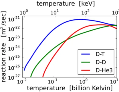
Figure 2: Reaction Rates of different fusion fuels dependent on the temperature... 4
Figure 3: CAD model of ITER... 6
Figure 4: cut through the cryostat ITER with important structures designated... 9
Figure 5: ITER Vacuum Vessel with locations of the ports... 11
Figure 6: CAD model of the CXRS Port Plug ... 12
Figure 7: Position of the CXRS Port Plug inside ITER... 14
Figure 8: Principle of Random Walk ... 18
-Figure 9: Neutron Path in Monte Carlo Simulation [BRIESMEISTER 03] ... 19
Figure 10: Neutron History in Monte Carlo Simulation ... 19
Figure 11: Working Flow of MCNP... 22
-Figure 12: Files used by FISPACT to produce a collapsed library [FORREST 05] ... 29
-Figure 13: Files used by FISPACT for a standard run [FORREST 05] ... 29
Figure 14: Radiation damage in aluminium in dependence of the fluence ... 35
Figure 15: Activity of some elements positioned near the first wall after ITER shutdown... 37
Figure 16: ITER Feat MCNP model ... 42
Figure 17: Analyzing single neutron trajectories with MCNP and SABRINA ... 43
-Figure 18: Plasma Region approximated by 5 Cells with uniform source in each layer [IIDA 06]... 44
-Figure 19: Vacuum Vessel in the ITER Feat model [IIDA 06] ... 44
-Figure 20: Divertor in the ITER Feat model [IIDA 06] ... 45
Figure 21: Dynamic CXRS model input sheet... 47
Figure 22: MCNP model of the CXRS Port Plug in ITER Feat model... 48
Figure 23: ITER CXRS PP MCNP model super positioned with a FMESH tally ... 49
Figure 24: Section of unformatted MCNP FMESH output ... 51
Figure 25: GUI of MOPAR with FMESH preview screenshot... 52
Figure 26: GUI of MOPAR with histogram of statistical errors... 53
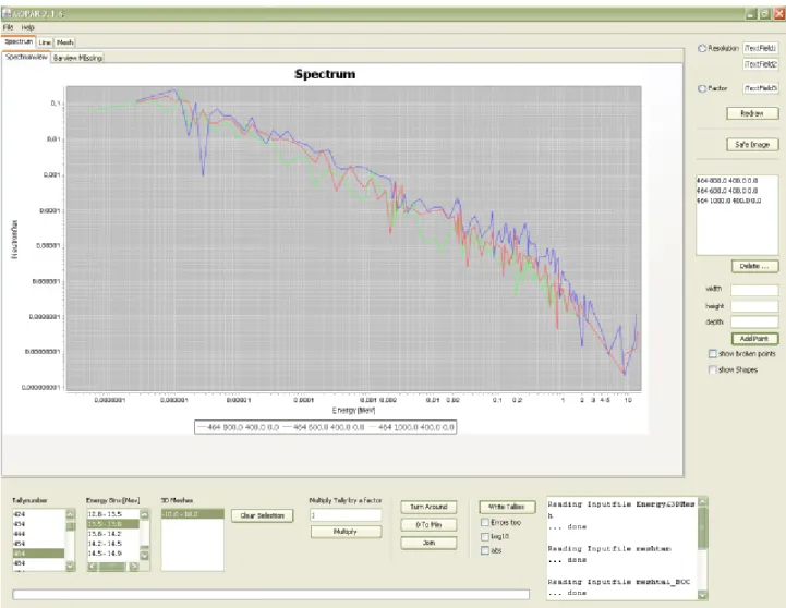
Figure 27: GUI of MOPAR with spectrum analysis of FMESH grid ... 54
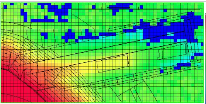
Figure 28: FMESH tally results with geometry plot visualized with 3DField after processing with MOPAR ... 55
Figure 29: Visualization of processed 3D Neutron Flux Data visualized with 3DField ... 55
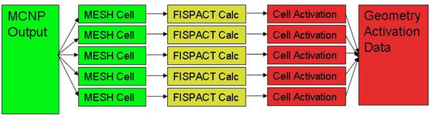
Figure 30: Cell based way of getting activation analysis for a complex MCNP model ... 56
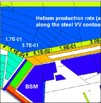
Figure 31: Visualization of Helium production in ECRH PP as part of activation analysis (FZK) ... 56
Figure 32: MESH based way of getting activation analysis for a complex MCNP model ... 57
Figure 33: Graphical User Interface of MCNPAct ... 58
Figure 34: MCNPAct: Combination of MESH data with geometry input data to discrete element files ... 59
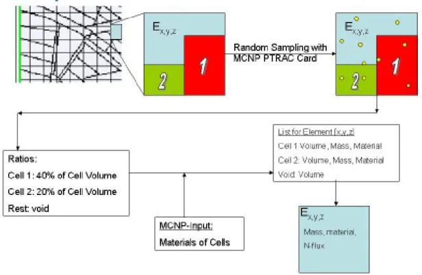
Figure 35: MCNPAct: Determining the element material composition by random sampling (example) ... 59
Figure 36: FISPACT computations and compilation of FISPACT output files to new matrix files ... 60
Figure 37: MCNPAct: Flowchart of the program modules ... 61
Figure 38: Abundance of iron in the MCNP input of ITER mapped over the geometry plot ... 68
Figure 39: 2D Map of a simple gamma source with 10x5x5 elements plotted over geometry. ... 72
Figure 40: Map of MCNP gamma transport calculation test results with automatically generated source... 72
-Figure 41: Plot of the newly modeled input based on the geometry used by [SHATALOV 02]... 75
-Figure 42: Results of the neutron flux verification model compared with [SHATALOV 02]... 77
Figure 43: Neutron Flux in ITER computed with ITER Feat model [log(n/cm²s)]. ... 78
Figure 44: Statistical error in ITER neutron flux calculation... 79
Figure 45: Gamma Flux in ITER computed with ITER Feat model [log(1/cm²s)]... 80
Figure 46: Line profile through the neutron flux distribution... 81
Figure 47: Line profile through the gamma flux distribution... 82
Figure 48: Neutron Flux in ITER CXRS PP [log(n/cm²s)]. ... 83
Figure 49: Neutron Flux in ITER CXRS PP at position of mirror 4 and 5 [log(n/cm²s)]. ... 84
Figure 50: Relative Neutron Flux Spectrum [MeV] at different locations in ITER CXRS PP ... 84
Figure 51: Line profile through the neutron and gamma heating distribution [W/cm³] ... 85
Figure 52: Neutron Heating in CXRS PP (log[W/cm³]) ... 86
Figure 53: Photon Heating in CXRS PP (log[W/cm³]) ... 87
Figure 54: Neutron flux along CXRS PP mirror labyrinth way of light [log(n/cm²s)] ... 88
Figure 55: Comparison with the neutron flux profile of NRG (FzJ/NRG) ... 90
Figure 56: Comparison with the heating profile of NRG (FzJ/NRG) ... 90
Figure 57: Superimposed image of the ITERFEAT (black) and ALiteMCNPmodel (red) ... 91
Figure 59: Heating values of the second mirror depending on the material chosen [W/cm³] ... 92
Figure 60: Results of the CXRS PP neutron flux calculations [n/cm²s] for the first mirror. ... 93
Figure 61: Results of the CXRS PP neutron heating calculations [W/cm³] for the first mirror... 93
Figure 62: CXRS PP photon heating [W/cm³] for the first mirror... 94
Figure 63: Neutron damage in CXRS PP in [log(dpa/FPY)]... 95
Figure 64: Material Damage in CXRS PP (2nd and 3rd mirror) in [log(dpa/FPY)] ... 96
Figure 65: Material Damage in CXRS PP (4th and 5th mirror) in [log(dpa/FPY)]... 96
Figure 66: Neutron Flux around the port plug [log(n/cm²s)] ... 97
Figure 67: Plot of the MCNP model without Port Plug ... 98
Figure 68: Neutron Flux in model without Port Plug [log(n/cm²s)] ... 98
Figure 69: MCNP plot of the ITER geometry used for the activation analysis ... 100
Figure 70: Activity of the most active isotopes inside ITER structures due to activation after shutdown... 101
Figure 71: Activity in ITER 1 day (left), 1 year (middle) and 10 years (right) after shutdown [log(Bq/kg)]... 102
Figure 72: Tritium content inside ITER structures due to activation after shutdown ... 103
Figure 73: Tritium activity in ITER 1 day (left) and 10 years (right) after shutdown [log(Bq/cm³)]... 103
Figure 74: W187 activity in ITER 1 day (left) and 30 days (right) after shutdown [log(Bq/cm³)] ... 104
Figure 75: Activation heat 1 day (left), 1 year (middle) and 10 years (right) after shutdown [log(kW/cm³)] ... 105
Figure 76: MCNP plot of the ITER CXRS Port Plug geometry used for the activation analysis ... 106
Figure 77: Activity in the CXRS PP 1 day (up) and 10 years (down) after shutdown [log(Bq/kg)]... 107
Figure 78: Co60 activity in the Port Plug one day after shutdown [log(Bq/cm³)]... 108
Figure 79: Tritium activity in the Port Plug one day after shutdown [log(Bq/cm³)] ... 109
Figure 80: Activation heat production 1 day (up) and 10 years (down) after shutdown [log(kW/cm³)]... 110
Figure 81: Dose Rate during operation due to gammas in ITER [log(rem/h)]... 111
Figure 82: Port Cell in MCNP model ... 112
Figure 83: Dose Rate due to activation gammas from Upper Port Cell structure in ITER in [log (rem/h)] ... 113
Figure 84: Helium Production in CXRS PP in [log (appm)] ... 114
Figure 85: Helium production in welded parts of the CXRS Port Plug ... 115
Figure 86: Geometry plot of the model used ... 116
Index of Tables
Table 1: ITER base parameters... 7
Table 2: CXRS measurement specifications ... 13
-Table 3: Estimated Error vs. Number of identical tallies [BRIESMEISTER 03] ... 24
-Table 4: Interpretation of the relative error [BRIESMEISTER 03] ... 24
Table 5: ITER main operating parameters... 30
Table 6: Heat loads specifications for ITER magnet system ... 31
Table 7: Radiation limits to ITER magnets ... 31
-Table 8: Area Classification and Radiation Access Conditions [IIDA 06] ... 32
-Table 9: Helium limits for different type weldings [IIDA 06]... 33
Table 10: Possible transmutation reactions for neutron energy < 15 MeV ... 36
Table 11: Steel to water ratios of different sources... 39
Table 12: List of materials foreseen for the ITER components ... 41
-Table 13: Results of the neutron flux verification model compared with [SHATALOV 02] ... 76
Table 14: Results of the CXRS PP neutron flux and nuclear heating calculations using MCNP ... 88
Table 15: Neutron Damage in CXRS PP in [dpa/FPY] ... 95
Table 16: Results of the computations for the coils... 99
Table 17: Activity of most active isotopes in ITER 10 years after shutdown... 101
Table 18: Activity of most active isotopes in ITER 1 day after shutdown ... 102
Table 19: Helium Production in CXRS PP in [appm]... 115
-Nomenclature
Symbols
h height [cm]
n number of neutrons generated [1/s]
r radius [cm]
t thickness [cm]
N number of neutrons, atoms [-]
R relative error [-] V volume [cm³] Φ neutron flux [1/cm²s] P power [kW] E energy [kWh], [eV] T temperature [°C], [°K], [eV] n plasma density [1/m³]
τ energy confinement time [s]
m mass [kg]
Q Plasma amplification [-]
B magnetic field [T]
H heat load [W/cm²],[W/cm³]
I electric current [A]
U electric voltage [V]
v velocity [m/s]
C concentration [%], [appm]
S standard deviation [-]
x population [-]
σ cross section [barn]
A activity [Bq]
D Dose [Sv], [Gy]
D/t Dose Rate [Sv/h]
t time [s],[a],[y], [fpy]
f fluence [MWa],[MWa/m²]
d radiation damage [dpa]
Indices E Energy confinement eff effective epi epithermal therm thermal fast fast stat statistical
Abbreviations
ACTL Activation Library ADL Activation Data Library
ALARA As Low As Reasonably Achievable ALARP As Low As Reasonably Practicable appm atomic parts per million
ASCII American Standard Code for Information Interchange BSM Blanket Shield Module
CAD Computer Aided Design CC Correction Coils CS Central Solenoid
CXRS Charge eXchange Recombination Spectroscopy CXRS Charge eXchange Recombination Spectrometer D1S Direct One-Step
DA Domestic Agencies DD Deuterium-Deuterium
DE Dose Energy
DEMO DEMOnstration Power Plant DNB Diagnostic Neutral Beam DT Deuterium-Tritium EAF European Activation File
EAST Experimental Advanced Superconducting Tokamak EASY European Activation System
ECRH Electron Cyclotron Resonance Heating ENDF Evaluated Nuclear Data File
ENDL Evaluated Nuclear Data Library FEM Finite Element Method
FENDL Fusion Evaluated Nuclear Data Library FNG Frascati Neutron Generator
fpy fusion power year FzJ Forschungszentrum Jülich FzK Forschungszentrum Karlsruhe GUI Graphical User Interface HFR High Flux Reactor
HHFC High Heat Flux Components IAEA International Atomic Energy Agency
IFMIF International Fusion Material Irradiation Facility IO Iter Organization
JENDL Japanese Evaluated Nuclear Data Library JET Joint European Torus
JUMP Juelich Multi Processor
JUROPA Jülich Research on Petaflop Architectures LANL Los Alamos National Laboratory
LLNL Lawrence Livermore National Laboratory
MC Monte Carlo
MCNP Monte Carlo n-Particle Transport Code MHD Magnetohydrodynamic
MOPAR MCNP Output Parser and Reckoner MPH (ITER) Material Properties Handbook MTR Material Test Fission Reactors NAR (ITER) Nuclear Analysis Report NEA Nuclear Energy Agency (France) NRG Nuclear Research and consultancy Group NRT Norgett-Ribinson-Torrens model
OECD Organisation for Economic Co-operation and Development PDE Partial Differential Equation
PDF Propability Density Function PF Poloidal Field
PP Port Plug
PP Port Plug
R2S Rigorous Two-Step
RSICC Radiation Safety Information Computational Center TEXTOR Tokamak EXperiment for Technology Oriented Research TF Toroidal Field
TFTR Tokamak Fusion Test Reactor
UKAEA United Kingdom Atomic Energy Authority UP3 Upper Port #3
UPP Upper Port Plug
VV Vacuum Vessel
1. Introduction
The Research Center Jülich is (FZJ) involved in the construction of the experimental nuclear fusion reactor ITER, an international enterprise to show that is technically and economically feasible to build thermonuclear reactors for energy generation. The Institute of Plasma Physics will design together with international partners the so called CXRS Upper Port Plug (CXRS UPP), a technical component, that will view directly into the fusion plasma and guide its light to the outside of the reactor chamber by a system of mirrors – much like a periscope - to a set of spectrometers, where the light is analyzed and crucial plasma parameters like density profile and plasma composition are determined.
As the CXRS UPP will be positioned directly in the shielding, facing the hot plasma where also high numbers of high energy neutrons will be created it is clear that a detailed neutronic analysis has to be made. All structures inside the reactor have to conform to ITER regulations, for example there are maximum numbers on certain parameters as helium production in welded parts or maximum nuclear heating in certain materials. Also it is important, that no other parts of ITER are endangered, as structures inside the shielding can lead to higher neutron fluxes outside. Especially the insulations of the magnetic coils are sensitive to neutron and gamma radiation, so there are limits again given by ITER regulations.
Of course there are limits not only due to regulations but also by the construction itself. Especially the first mirror in the CXRS Port Plug is facing directly the plasma and is subject to high neutron fluxes as well as high neutron and gamma heating. So it is important to determine the exact amount of these quantities, so that construction is optimized for these loads. Values for neutron flux, neutron and gamma heating and also material damage should be determined for any point in the geometry. Also it is important to make an activation analysis of the component to determine the activation, activation heating and the composition and masses of activation products and its radiation dose rates at certain times of ITER operation, especially after shut down, when workers are supposed to have access to some areas of the reactor interior.
Because of availability and good experiences these calculations should be done with the Monte Carlo Code MCNP and the activation code FISPACT. MCNP is capable of using three-dimensional models with a high amount of detail and it can be run on the Jülich JUMP and JUROPA supercomputers in parallel mode to reduce the computation time. FISPACT is an activation code, especially developed by UKAEA for fusion problems.
There are some challenges associated to these tasks. One point is the high complexity of the geometry not only for ITER but also for the Port Plug. As modelling in MCNP is not possible by a GUI but is happening manually by including mathematical surfaces and cell descriptions in a ASCII input file, ways had to be found to simplify the workflow when modelling,
especially as model modifications had to be made in short time due to the nature of the design process.
As MCNP is capable of determining a lot of data in one model, some ways had to be found to prepare these data for easy analysis and interpretation. Usually MCNP and FISPACT are giving computed data in the format of output text files. Solutions had to be made to compile these text files into some useful mode of visualization.
Another challenge was the workflow of using MCNP simulation results as inputs for the FISPACT code. While MCNP is able to give data for three-dimensional models, FISPACT is working zero-dimensional. When using FISPACT for complex structures, several runs have to be made to get distributions. There are in fact codes to forward MCNP results for single cells to FISPACT, so that activation data can be achieved for single MCNP cells, but there are disadvantages with respect to spatial resolution and also visualization capabilities when using this method, so an alternative method should be developed to get activation data for all points of a model in any resolution.
These newly to developed methods should be made in a general form, so that any geometry not only the CXRS Port Plug can be simulated with them. Finally the methods should be applied to the Port Plug and the results had to be compared to that of other groups for verification purposes.
2. Nuclear fusion principles & ITER description
2.1.
Nuclear Fusion
More than ninety percent of the world’s energy consumption is won from fossil energy sources: mostly by coal, petrol and gas. Limited resources and questions about the climate change demand a discussion about the origin of the energy in the future. The problem will get more critical by the increasing world population and the higher need for energy [COENEN 09].
All over the world energy research is looking for alternatives to the fossil energy sources. There is a broad spectrum of possibilities for the future and the rising contributions by regenerative energy sources like wind power and solar electric power are first steps on the road. Nuclear fusion is the vision of realising the application of the sun’s energy here on earth. Its promise is a save and almost unlimited source of energy. From the nuclear fusion of one gram of deuterium and tritium it is possible to get 26,000 kWh of energy what is equal to the energy won from 11 tons of coal. In the long term, nuclear fusion is the only option. Humanity will suffer if researchers don’t solve its problems. [SEIFE 08]
As the tritium is won from lithium by breeding inside the reactor, and the lithium is processed from stones, it is possible to deliver the energy needed for a family in one year by two litres of water and half a pound of stones. The world’s energy consumption could be covered by the natural resources of deuterium and lithium for ten thousands of years.
Furthermore a fusion reactor would be inherent safe. No chain reaction is possible as the amount of fusion fuel in a reactor at any given time is very low and also no climate endangering gases like carbon dioxide are emitted.
In a fusion reactor light nuclei are more plentiful than fissile nuclei, and thus there would be much less radioactive waste from a fusion reactor than from a fission reactor. Furthermore, any radioactivity would decay away rapidly and there would be no need to store the waste for geological periods of time. [LILLEY 01][HULME 69]
Aim of the world’s fusion research projects is the development of the plasma physical basics and also to get the technical knowledge of designing a workable fusion reactor.
Figure 1: nuclear Fusion of Deuterium and tritium
Nuclear fusion gets its energy from the same origin than nuclear fission: the binding energy of the nuclear core. If two light atoms are fused to one heavier core, a part of the binding energy is transferred to kinetic energy. Figure 1 shows the mechanism for deuterium and tritium, which are transformed by fusion to a helium atom and a neutron. The excess energy amounts to 17.6 MeV from which the most part is carried away by the neutron. While the helium is supposed to give its energy to other nuclei for sustaining the fusion reaction, the neutron carries its energy to the outside where it can be used by thermal conversion to electric energy. [BRÖCKER 97] There are several fusion reactions suitable for energy generation, the most important are shown in Figure 2. From the ones shown, the deuterium-tritium reaction has the highest reaction rate at temperatures of about hundred million degrees Celsius, which are reachable today.
To get fusion reactions, the atoms must have a certain kinetic energy as they have to overcome the Coulomb barrier, which has the effect of a repulsing force up to a certain distance from the core. Once the Coulomb force is surmounted, the strong nuclear force will gravitate the atoms to each other and fusion will occur. The needed initial kinetic energy will be reached by heating the fusion fuel to a plasma inside a toroidal vacuum chamber, called a tokamak. Some hundred million degrees Celsius are realizable today by holding the plasma with magnetic fields to prevent cooling by contact with the wall.
The technology of heating the fuel in a plasma is called magnetic confinement fusion. There are other options researched today, like the inertial confinement fusion or the Z-pinch method, but these are not of relevance for this work. [GLASSTONE 64]
The energy released by the fusion reaction is shared between the alpha particle, with 20% of the total energy, and the neutron, with 80%. As the neutral neutron will leave the plasma immediately, only the energy of the alpha particle will contribute to the heating of the plasma. To get rid of the need for external heating, the temperature of the plasma must be high enough for the rate of the alpha particles to sustain the fusion reaction in the reactor by themselves. [KAMMASH 75][RAEDER 81]
The condition for this ignition in magnetic confinement is calculated by setting the alpha particle heating equal to the rate at which energy is lost from the plasma. The ignition condition has the same form as the Lawson criterion [LAWSON 57]. The product of density and confinement time must be larger than some specified value, which depends on the plasma temperature and has a minimum value in DT at about 30 keV. The condition for ignition is nτE > 1.7E+20 m-3s
where τE is the energy confinement time that gives the rate at which energy is lost from a
plasma. In a steady state working reactor, τE is a measure for the quality of the magnetic
confinement. [MCCRACKEN 05]
As the fusion cross sections and some other parameters depend on temperature, it turns out that the most suitable temperature range is between 10 and 20 keV. The ignition condition can also be written in a form called ‘triple product’, which includes the temperature:
nTτE > 3E+21 m-3skeV
For magnetic confinement fusion, an energy confinement time of about 5 seconds and a plasma pressure of about 1 bar is one combination that could meet this condition.
The earliest magnetic-confinement devices were developed in the UK in the late 1940s. These were toroidal pinches, which attempted to confine plasma with a strong, purely poloidal
magnetic field produced by a toroidal plasma current, but this arrangement proved seriously unstable. [MCCRACKEN 05]
The second approach to toroidal confinement is the stellarator, invented at Princeton in the early 1950s. Here a strong toroidal magnetic field is produced by an external toroidal solenoid. But here it is necessary to twist the magnetic field as it passes around the torus, what results in complicated coil shapes. Advances in physics and engineering are resulting in further experiments like the W7-X machine at Greifswald.
The most successful toroidal confinement scheme is the tokamak, developed in Moscow in the 1960s. The tokamak can be thought of either as a toroidal pinch with very strong stabilizing toroidal field or as using the poloidal field of a current in the plasma to add the twist to a toroidal field. ITER will be a tokamak type fusion reactor. [MCCRACKEN 05]
2.2.
ITER
ITER – once the abbreviation for International Thermonuclear Experimental Reactor, today simply the Latin translation of ‘the way’ is the international research and engineering proposal for an experimental project that will help to make the transition from today's studies of plasma physics to future electricity-producing fusion power plants. It will build on research done with todays devices such as DIII-D, EAST, TFTR, JET, TEXTOR, and will be considerably larger than any of them. A simplified 3D CAD sketch of ITER with the most important components designated can be seen in Figure 3.
Fusion scientists are convinced that the main goal will be achieved: the generation of a burning fusion plasma, which will be showing the availability of a controllable nuclear fusion. While the physical laws of the plasma conditions are known to a sufficient degree, there are still a number of unsolved technical and engineering problems. This is mainly because there are demands to a full scale nuclear fusion power plant, which are playing no role in today’s experimental machines.
While fusion plasmas are only of short duration in existing tokamaks, there must be a constant burning in an economically working fusion plant. This will result in enormous challenges to the machines structures and components to withstand these loads. Even while ITER is “only” generating an eight minute fusion plasma, it will do so at power outputs in a power plant scale and is an ideal test bed for materials and techniques needed for full scale power plant construction.
Table 1: ITER base parameters
The main operational parameters of ITER are shown in Table 1. The fuel for ITER will be a deuterium-tritium mixture to react to helium with the reaction
D + T -> He4 + n
In future fusion devices it is planned to generate the radioactive tritium by nuclear breeding reactions. For this there will be a certain amount of lithium6 in a so called breeder blanked near the first wall of the plasma. The fusion neutrons will the react with the lithium atoms to tritium in the reaction
Li6 + n -> T + He4 and
Li7 + n -> T+ He4 + n
In ITER the tritium will be produced external. But the techniques of the breeding components will be tested in special modules near the first wall.
Apperture Radius 10,7 m Apperture Height 30 m Plasma Radius 6,2 m Plasma Volume 837 m³
Plasma Mass 0.5 g
Magnetic Field 5.3 tesla
Heating Power 73 MW
Fusion Power 500 MW
Temperature 1E+8 K
Originally planned due to an international initiative by the statesmen Gorbatschow, Reagan and Tanaka in 1986, it was supposed to have a fusion power of 1500 MW. After a change in the US research politics, the USA receded from the program. The other partners EU, Russia and Japan reacted by downscaling ITER to a output power of 500 MW.
ITER will be produced largely through in-kind contributions from the ITER members. The responsibilities for the management of in-kind procurement activities is assigned by each member to entities called domestic agencies (DA). During the same period that ITER Organization (IO) was established at the Cadarache site, the domestic agencies were set up. Today the ITER site has been cleared and work has started on the basic infrastructure. Also, construction of major components has started in the DAs. [HOLTKAMP 09]
The machines main goal is a burning fusion plasma of eight minute duration and an energy amplification of at least Q=10. These parameters will allow new physical examinations, like alpha-heating mechanism and analyzing instabilities that will limit the operational borders in certain plasma density and plasma pressure boundaries.
With some operational schemes it should be possible to extend the burning time of the plasma to 30 minutes by implementing a plasma flow operation with a combination of induction and high frequency energy input. This operation mode is important, as it will simulate a constant operation of a fusion reactor.
During its lifetime, ITER will be operated in successive phases. First phase is the H-Phase. In this non-nuclear phase only hydrogen or helium plasmas will be ignited, mainly for commissioning of the tokamak-system in a non-nuclear environment, where no remote handling procedures are needed. Second phase is the D-Phase, where deuterium plasmas are used. As the characteristics of deuterium plasmas are similar to that of DT-plasmas, this phase is ideal for simulating the procedures and operations of the DT-phase. During the DT-phase, the fusion power and burn pulse length will be gradually increased until the operational goals are reached.
ITER is a long pulse tokamak with elongated plasma and single null poloidal divertor. The major components of the tokamak, as depicted in Figure 4, are the superconducting toroidal and poloidal vacuum vessel. The magnet system comprises toroidal field (TF) coils, a central solenoid (CS), external poloidal field (PF) coils and correction coils (CC). The TF coil windings are enclosed in strong cases used also to support the external PF coils.
ITER has one of the largest and the most complex high vacuum system ever. Reliable vacuum is the key to the success of the ITER project. Due to the extensive nature of the ITER vacuum there are very few ITER systems which will not have an important vacuum interface. [ITER 08]
Figure 4: cut through the cryostat ITER with important structures designated
The vacuum vessel is a double-walled structure, made of a stainless steel welded ribbed shell, with internal shield plates and ferromagnetic inserts to reduce toroidal field ripple and is also supported by the toroidal field coils. The magnets together with the vacuum vessel are
supported by gravity supports. Inside the vacuum vessel, the internal components including blanket modules, divertor cassettes and port plugs absorb the radiated heat as well as most of the neutrons from the plasma and protect the vessel and magnet coils from excessive nuclear radiation.
The 421 blanket modules have a single-curvature facets separate first wall attached to the vessel through 3 cm diameter access holes in the first wall. The plasma facing components are beryllium armour attached to a copper substrate, mounted on a water-cooled stainless steel support. The outboard modules may later be replaced with tritium-breeding modules.
The 54-cassette single null divertor has carbon targets and tungsten high heat flux components, mounted on a copper substrate bolted to rails on the vessel floor. These targets can accommodate heat loads of more than 20 MW/m² for 20s, but the normal peak heat load will be 5 to 10 MW/m².
Equatorial and upper port plugs are used for heating antennae and neutral beam ducts and diagnostics. Divertor ports are housing torus cryopumps, diagnostics, cleaning systems and are also used for remote replacement of the divertor cassettes.
The heat deposited in the components of ITER is rejected to the environment by means of the tokamak cooling water system designed to exclude releases of tritium and activated corrosion products. The entire tokamak is enclosed in a cryostat, essentially a cylinder 24 m high and 28 m diameter, with thermal shields between the hot components and the cryogenically cooled superconducting magnets. [ITER01][THOMAS 07]
The ITER design status is far from closed. Results from running experiments and design studies as well as changes in the demands to the physics experiments are resulting in constant modifications of the ITER specifications. The maximum operating density, auxiliary heating power and the criteria to achieve a certain mode of confinement defines the operating space for the baseline 15 MA, 5.3 T scenarios. The baseline heating power is 73 MW and could be further increased if necessary.
In the last years several further changes have been made to the original design. The core parameters were reaffirmed and many detailed issues were addressed to ensure that ITER would meet its mission requirements. The poloidal field coil was modified to ensure that the plasma can be adequately controlled. Stabilization of a vertical disruption event was addressed by including in-vessel coils and the vacuum vessel was changed as a result of recognizing the implications of prior results on JET and associated modelling. [HAWRYLUK 09]
2.3.
ITER Diagnostics and CXRS Upper Port Plug
Figure 5: ITER Vacuum Vessel with locations of the ports
The implementation of diagnostics on ITER will be a major challenge, as the environment will be much harsher than in existing reactor experiments. For example the levels of neutral particle flux, neutron flux and fluence will be respectively about 5, 10 and 10,000 times higher than in today’s machines.[COSTLEY 01]
ITER diagnostic equipment is integrated in six equatorial and 12 upper ports, five lower ports, and at many other locations in the vacuum vessel, as seen in Figure 5. The integration has to satisfy multiple requirements and constraints and at the same time must deliver the required performance. [WURDEN 97]
To control and evaluate plasmas on ITER it will be necessary to measure the plasma current in the range of 1 – 20 MA with an accuracy of 1%; the plasma shape and position to a few cms; the loop voltage to within a few mV, the plasma energy to < 10%, and the amplitude of MHD modes to typically 10%. The measurements are required with a time resolution of < 10 ms and for pulse lengths of up to 3,600 s.
Another important parameter to be measured on ITER will be the fusion power and related parameters such as the neutron flux and emissivity, neutron fluence and ion temperature. For the control and evaluation of ITER performance these are required to an accuracy of 10% with good temporal and spatial resolution.[COSTLEY 01]
The CXRS (Charge Exchange Recombination Spectroscopy) upper port viewer for ITER is an active diagnostic measuring light from the interaction of the charged plasma particles with the ions of a neutral beam (DNB). [SADAKOV 09]
Parameters to be measured are temperature profile, Helium ash density profile, Impurity density profile, plasma rotation, alpha particle confinement. The system will be installed at the upper port for measurements in the plasma core region. The CXRS system consists of the following subsystems: Collecting and re-imaging optics, fibre optic channels, spectrometers, detectors and data-acquisition. A CAD drawing of the CXRS Port Plug is shown in Figure 6. [KONING 09]
Figure 6: CAD model of the CXRS Port Plug
Light emitted from the ITER plasma is collected by the front optics system. The light is guided through a labyrinth and imaged on the entrance surface of a bundle of fibre optic waveguides. Through the fibre optic waveguides the light is guided to a set of spectrometers of different types.
The instrument will be installed in a port plug in diagnostic upper port #3 (UP3). The upper port plugs are installed in the ITER Vacuum Vessel (VV) and include a plasma-viewing first wall blanket shield module. Required mirror diameters are in the order of 35 cm which fits within the available cross-section of the port plug.
The measurement requirements of this system are summarized in Table 2. To achieve these, a 3.6 MW, 100 keV hydrogen diagnostic neutral beam (DNB) is foreseen. [JASPERS 08]
Parameter Range Time resolution Space resolution Accuracy
Helium density 1-20% 100 ms a/10 10%
Ion temperature
0.5 - 40
keV 100 ms a/10 10%
Poloidal plasma rotation 1-50 km/s 10 ms a/30 5 km/s - 30 %
Toroidal plasma rotation 1-200 km/s 10 ms a/30 5 km/s - 30 %
Impurity concentration Z<10 0.5 - 20 % 100 ms a/10 20%
Impurity concentration Z>10 0.01-0.3 % 100 ms a/10 20%
Table 2: CXRS measurement specifications
However, design issues are seriously increased due to the following facts: The high amount of radiation in the front of the port plug precludes the use of transmissive elements, so that at the front opening only reflective optics can be used.
The first mirror is exposed to a high neutron and heat load and is in an environment where deposition of carbon is likely. Both leads to a high degradation rate of the first mirror and therefore protective measures are required to ensure the lifetime of the first mirror. Also the first mirror is exposed to large heat transients at the beginning of operation that may create a change in curvature of the mirror surface.
The mirror material is one of the most important parameters to determine the rate of degradation. Presently the most likely option is to use a mirror made of mono-crystalline molybdenum.
Furthermore, the mirror shall be placed in a retractable tube in order to be replaced after a while and a shutter will enable protection when CXRS is not functional between the shots. The shutter and the exchange construction are both mechanical moving systems. They should be simple in order to guarantee functionality.
The shutter is a movable element located in a harsh nuclear, vacuum and electromagnetic environment: volumetric heat up to 3 W/cm³, surface heat up to 1 W/cm². Poloidal magnetic field variation rate in the gap between plasma and FW reaches up to 120 T/s.
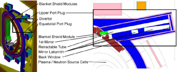
Figure 7 shows the position of the CXRS port plug inside the ITER reactor and the principle layout of the instrument. In order to separate the mechanical systems from the optical labyrinth, the periscope has been divided in a mechanical and an optical layer.
The mechanical layer resides in the upper part of the periscope and consists of mirror #1, the shutter mechanism and the replacement system. The optical layer resides in the lower part of the periscope and consists of all optical elements except for mirror #1.
Figure 7: Position of the CXRS Port Plug inside ITER
The BSM is different from the standard blanket concepts, because it needs to have apertures and is attached to the port plug and not to the vessel.
The main shell encloses and supports the “shielding cassette” which, in turn, encloses and supports the retractable tube. The shell has a closed cross section which maximizes the stiffness and allows local round access hatches for adjustment and replacement of the secondary mirrors. In the reference design the shell also carries the blanket shield module, but this might be reconsidered.
The shielding cassette forms optical channel, holds the retractable tube and the secondary mirrors. It also has an endoscope channel for the inspection of the 1st mirror and calibration. The cassette holds main water pipes at the rear flange and delivers the cooling water to all other components of the plug including the main shell.
The rear flange is congested with allocation of tube’s flange, optical channel, main water pipes and smaller pipes connecting the tube with the cassette, and a docking area for remote handling cask for tube replacement. Secondary mirror holders are located at side or bottom surfaces. Round hatches for the mirrors at the bottom surface of the shell is the preferred option.
Behind the Port Plug, a fibre bundle transports the light over tens of meters to the spectrometer room. For the spectrometer and the detection systems several options are yet under study to arrive at a system measuring simultaneously four wavelength bands. [JASPERS 08]
Possible technical solutions for the CXRS plug were developed. The major efforts have been spend on the resolution of three critical problems. The first problem is the uncertain and likely short lifetime of mirror one. A relocation of the mirror to a bigger distance from the front wall would be suggested. Second task is the development of a robust and efficient shutter in the
harsh environment. Specific design utilizes elastic bearings and pneumatic actuators. A further problem is the BSM to Plug Plug attachment. A robust design should have good margins for eddy current and halo loads. [SADAKOV 09]
Nuclear analysis is required for the licensing of the Port Plug. Of interest are the neutron and gamma fluxes throughout the Port Plug geometry and especially the neutron flux and nuclear heating at the mirrors. The effect of port plug leakage on neighbour relevant ITER systems must be studied. [WALKER 03]
3. Theoretical basis and standard methods
3.1. Nuclear fusion neutronics
In a fission reactor, approximately one neutron gets released for each 80 MeV of fission energy, and the average energy of fission neutrons is about 2 MeV. In a deuterium-tritium based fusion reactor, one neutron is released per 17.6 MeV of fusion energy, and the fusion neutrons have initially a kinetic energy of about 14.1 MeV. [WASASTJERNA 07][STEPHENSON 58]
With other words, the sole number of neutrons released per energy unit is higher by about a factor of four and the energy of the single neutrons is higher by about a factor of seven. In contrast to fission reactors, neutrons are not needed for sustaining a chain reaction, but neutrons are needed nonetheless for breeding the tritium and carrying the energy from the plasma to the wall, where the neutron kinetic energy is transferred into thermal energy for conversion into electricity.
But the thermal energy, deposited by the neutrons in the material will also be responsible for stresses in the structure. Furthermore the neutrons will generate gamma radiation by collisions with other nuclei, which also will be carrying heat to other regions. Both of them, neutrons and gammas will also be responsible for radiation damage, when colliding with atoms, knocking them out of their metal lattice. All these processes have to be calculated and analyzed by neutron simulation codes to help the engineers in designing the structures, shielding, cooling systems.
Further neutrons will be getting absorbed by atoms of the structures and activate the material, transferring it to another isotope or element by transmutation. Optical elements will degrade by these processes; other materials will get radioactive, emitting gamma radiation even after shut down of the machine. Activation will also produce hydrogen and helium, what can be fatal for welded parts. Also these processes have to be computed and analyzed with activation codes to design the reactor in a way that radiation limits can be guaranteed. [CHENG 00],[ERIKSSON 03] In principle, shielding calculations, like other neutronics calculations, can be performed using either deterministic or Monte Carlo methods. However, deterministic methods have difficulties in coping with the geometrically-complex mixture of shielding materials and voids typical of ITER and presumably other fusion reactors. Typically they use one or the other of two opposite methods of representing the angular dependence of the flux. The SN method and the method of characteristics use a limited number of discrete flight directions. The PL method expands the flux in terms of Legendre polynomials of the angular variables. The former method is plagued by ray effects when applied in voids, and the latter introduces a spurious angular spreading. [WASASTJERNA 07]
Discrete ordinates codes (Sn) used in fusion to date were only 1D oder 2D and even greater geometrical simplifications led to the need for confirmation of the results using MC methods. A 3D discrete ordinate tool based on direct CAD input exists nowadays which, whilst preserving geometrical detail, provides fast evaluation capability and practical post-processing tools. This tool, the Attila 3D Sn code, is actually studied in fusion applications with respect to its performance, functionality and results.
Different evaluations still show a series of issues regarding the functionality and methodology. For example preparations of appropriate CAD inputs proved to be very challenging, but good agreement with MC methods were also achieved. [PAMPIN 07]
Several approaches have been made in the past to combine the advantages of the deterministic and the Monte Carlo codes and use the MC advantages for the interior of the reactor and to compute the shielding problem with deterministic codes. This can be achieved by coupling of different codes like MCNP5/MCNPX with ANISN, DORT or TORT. [HANSLIK 06],[CHEN 05] Computations to determine the neutron and gamma flux and the accompanying dose rates within the ITER building but outside the cryostat, where low numbers are expected, have been done with these coupling methods. [EGGLESTON 98]
In this work we relied on the Monte Carlo method, which is capable of handle material filled cells as well as large voids in three-dimensional geometries. Reliability of the results is mostly dependent on the number of particle trajectories calculated. In large and complex structures like ITER it can sometimes be hard to get good statistics, as discussed later, but variance reduction methods can help in saving computation time.
3.2.
Fundamentals of the Monte Carlo Method
The Monte Carlo method provides approximate solutions to a variety of mathematical and physical problems by performing statistical sampling experiments on a computer. A classic use is the evaluation of definitive multidimensional integrals by random sampling which is extensively utilized in the field of particle transport. [FISHMAN 95]
In this connection Monte Carlo may be considered as a means of repeatedly applying interaction probability data to individual particles selected randomly until a sufficient number of particles have been observed to allow conclusions to be drawn concerning the macroscopic multicollision behaviour of the total population of particles within a material region.
The rise in calculating capacity of recent supercomputers has made MC Methods very common today. MC is also used in other applications like illumination computations which produce photorealistic images of virtual 3D-Models (ray tracing). They are useful in studying systems with a large number of coupled degrees of freedom, such as liquids, disordered materials, and
strongly coupled solids. They are also used for modelling phenomena with significant uncertainty in inputs, such as the calculation of risk in operational research. [BRIESMEISTER 03]
Figure 8: Principle of Random Walk
To understand the principle of stochastic methods, it is important to know about the elementary concepts of probability, namely, that the probability of one of several possible events occurring will be approximately equal to the ratio of the number of times the desired event occurs to the total number of events observed in an unbiased manner. As the number of observations increases, this ratio should more closely approximate the true probability.
Much of the information available on the physics of individual nuclear interactions is obtained experimentally by observing the fate of large numbers of particles. So, MC may be considered as a means of repeatedly applying interaction probability data to individual particles selected randomly until a sufficient number of particles have been observed to allow conclusions to be drawn concerning the macroscopic behaviour of the total population of particles.
Although Monte Carlo may be considered a means of solving the Boltzmann transport equation, it is more properly a modelling of the physical principles from which the Boltzmann equation was developed.[SCHAEFFER 73]
Simply stated, the Monte Carlo approach requires the construction of case histories of the travel of individual particles through the geometry and then analyzes these histories to derive relevant data, such as flux density and dose rate. One particle history includes birth of a particle at its source, its random walk (Figure 8) through the transporting medium as it undergoes various interactions, and its death, which terminates the history. A death can occur when the particle becomes absorbed, leaves the geometric region of interest, or loses significance to other factors (e.g., low energy). [SCHAEFFER 73]
Single particle histories inside any given 3D geometry are simulated like shown in Figure 9. In this example a random neutron incident takes place inside a block of fissionable material. The neutron enters the material coming from an (simulated) void and collides at event 1. The neutron is scattered in the direction shown, which is selected randomly from the physical scattering distribution. A photon is also produced and is temporarily stored for later analysis. Fission occurs at event 2; the incoming neutron is terminated while two new, outgoing neutrons and one photon are generated. One photon and one neutron are again temporarily stored for later analysis.
Figure 9: Neutron Path in Monte Carlo Simulation [BRIESMEISTER 03]
The first fission neutron is captured at event 3 and terminated. The second, stored neutron is now retrieved and, by random sampling, leaks out of the material cell at event 4. The photon that was created in the fission process has a collision at event 5 and leaks out at event 6. The photon from the first collision is now retrieved. It undergoes capturing at event 7. This was now one complete neutron history. More of such histories, millions of them, are followed to make a better distribution 0. A more detailed description on the background of this process is described in the following lines.
Figure 10: Neutron History in Monte Carlo Simulation
If the problem geometry is accordingly modelled, the major steps involved in generating a particle history are shown in Figure 10. The loop is continued until the particle parameters fall outside certain limits, such as geometrical bounds or minimum energy .The first three
operations displayed in the picture involve the selection of parameters at random from a probability distribution of all possible values of these parameters. The steps in making a random selection from such probability distributions are based on the use of numbers randomly positioned between 0 and 1.
All physical processes, including the emission of radiation and their subsequent transport through material, are probabilistic. It’s not possible to predict with certainty the destiny of an individual particle in a process. But it’s possible to characterize effectively these stochastic processes by describing the average behaviour of many elements or by estimating with a known degree of confidence the behaviour of one single element.
Inherent in the Monte Carlo procedure is the concept of the probability density function (PDF). This function describes the relative frequency of occurrence of its random variable x out of its domain (all possible values for x) constituting the event space (all possible events in the process). The random numbers needed may be taken from tables called into the machine memory or they may be generated by a subroutine of the MC computer program.
The first step in starting a particle history is the choosing of the source parameters. The source parameters include the energy, the spatial point of origin and the direction of motion. These parameters can be independent or may be interrelated with each other. The source energy is usually chosen from a given energy distribution. Same is true for the spatial distribution. Usually the user is giving coordinates as a starting point for the histories.
If a whole region in the model is designed for starting particles, the starting points will be chosen randomly within the coordinate limits of this region. If the sources are emitting particles isotropically, the program is simply picking unit vectors terminating uniformly on the surface of a unit sphere. The probability function (PDF) would then be the integral over a spherical surface area.
In certain calculations it may be desirable to prejudice the selection of one or more source parameters to favour those most likely to contribute to the quantity of interest. This can be done by selecting a larger number of the important source particles and assigning each particle a weighting number to adjust for the bias that was introduced.
The next step, if particle generation is complete, would be the determination of the particle path length from the source to the point of interaction. The path length together with the parameters of initial direction defines the point where an interaction occurs. If now the path length of the particle L is larger than the geometrical limits of the system A, the particle history will be terminated. Otherwise a collision or interaction is assumed to have occurred at the selected point and the collision parameters will be calculated.
If a collision has been detected it is necessary to determine, which of the possible nuclear species (if the material consists of multiple elements or isotopes) was involved and which
interactions of that species took place. For that the interaction cross sections must be available to the computer for each nuclide over the energy range of interest. These cross sections are usually stored in external databases, but more on this subject is mentioned, when the MCNP program is described in the next chapter.
For neutrons the possible reactions and therefore the necessary cross sections would be usually elastic scatter, absorption, fission, (n,n’), (n,2n) and (n,3n). The occurring reaction is then simply chosen by the computer program by selecting randomly according to the probability of that reaction. Secondary neutrons would be included by tracking them after the history of the incident neutron is terminated.
The next task is the determination of the parameters of the particles that survive an interaction. These parameters include the type, number, energy, and direction of the surviving incident particle and of any secondaries created. Depending on the type of data needed it may be useful to determine the energy stored in the material during the collision.
After the particle termination, that could be the result of absorption or due to low energy or the leaving of the system boundaries, the scoring takes place. The scoring is the output of a Monte Carlo simulation that can include the following results:
- Flux density as a function of position, direction and energy deposition - The penetrating dose or flux density
- The energy and angular distribution of the penetrating particles
- The distribution of penetrating particles relative to the number of collisions encountered before penetrating
- The distribution in time of arriving particles Many other possible data are thinkable for collection.
The Monte Carlo technique has been proven useful in special cases, such as complex geometries where other methods encounter difficulties and in some cell calculations. Moreover, when there is considerable detail in the variations of the neutron cross section with energy, the MC method eliminates the necessity for making subsidiary calculations, e.g., of resonance flux. [BELL 70]
In 1930 physicist Enrico Fermi used MC methods to calculate the properties of the newly-discovered neutron and these methods were central to the simulations required for the Manhattan Project. Extensive use was made after 1945, when the first electronic computers were built. At that time MC methods began to be studied in depth and became popular in the fields of physics and operations research. [NORDLUND 06]
3.3.
The MCNP computer code
MCNP (Monte Carlo n-Particle Transport Code) is widely used for this type of nuclear calculations. Furthermore in the ITER project, the MCNP code has been chosen as a standard, as it is versatile, accurate and well-tested program. [WASASTJERNA 07]
MCNP was originally developed by the Monte Carlo Group, currently the Radiation Transport Group, at the LANL (Los Alamos National Laboratory). MCNP is constantly improved and maintained and there is limited consulting and support for users. MCNP is distributed to users through the Radiation Shielding Information Center (RSICC) at Oak Ridge, USA and the OECD/NEA data bank in Paris, France.
MCNP (Version 4B) consists of approximately 40,000 lines of FORTRAN and 1000 lines of C source code. Worldwide, there are about 1000 active users.
MCNP takes advantage of parallel computer architectures. It has been made as system independent as possible to enhance its portability, and has been written to comply with the ANSI FORTRAN 77 standard. With one source code, MCNP is maintained on many platforms including UNIX, LINUX and Microsoft Windows.
Figure 11: Working Flow of MCNP
Figure 11 shows the typical work flow of a MCNP run. The user first has to create one or more input files that specify the problem to be calculated. The input includes definitions of the geometry, the properties of the materials used, and links to the files with the cross sections, particle sources information and many other things.
For the calculation of the reactions, MCNP uses external cross section files. These are continuous-energy nuclear and atomic data libraries. The primary sources are evaluations from the Evaluated Nuclear Data File (ENDF) system, the Evaluated Nuclear Data Library (ENDL) and the Activation Library (ACTL) compilations from LLNL (Lawrence Livermore National Laboratories), USA.
Nuclear data tables exist for neutron interactions, neutron-induced photons, photon interactions, neutron dosimetry or activation, and thermal particle scattering. Photon and electron data are atomic rather than nuclear. Over 500 neutron interaction tables are available for approximately 100 different isotopes and elements.
When the MCNP program is started, it begins with checking the input files. If no errors are found the particle histories are started. In fissionable materials MCNP can determine all the starting points alone, from which neutron paths can be randomly started. Also it determines the keff factor of the geometry, when fissile material is abundant. The histories of the particles
together with all other desired data are written from the program into output files. The user then can analyze the data and modify the input if necessary or the last run can be continued if the accuracy of the output has to be raised. MCNP geometrical nodalization
The largest part of the MCNP input file is mostly the definition of the problem geometry. MCNP geometry works with different 3-dimensional cells, consisting of a defined material. A cell is defined in MCNP by a composition of different surfaces in spaces. If the user wants to create a cell with the shape of a cube, he has to give the parameters of the six surfaces, which are the borders of the cube. More complex geometries are composed out of additions and/or intersections of simple geometrical objects.
For new users this way of dealing with geometries is somewhat difficult but with some training this works very well. MCNP is supporting the user by the possibility to plot 2D pictures of the geometry on the screen what is a help for the debugging of the input.
To get overviews of more complex geometries it can help to get three dimensional pictures of the input file. This is possible with an external tool with the name SABRINA. [VAN RIPER 06] The program has been used several times in this work for visualization of complex models. Furthermore it is possible to insert particle paths into the geometry. There are also some other more complex methods for scanning the model with the help of the MCNP source routine in order to visualize the material cells. [SNOJ 09]
The cells have to be assigned now to specific materials. The composition of the material is given by a nuclide identification number, the so called ZAID, and the weight fraction or nuclide fraction of it in the material. The ZAID links to the external data file with the cross sections of the nuclide. The user has to take care, that the given data files are accessible in the MCNP directory.
When all material and nuclear data files have been chosen, the user has to define the quantities of interest. They are called “tallies” and can be whatever one wants to know. One tally could be the number of neutrons, at certain energies, that entered certain cells or surfaces. Another tally could be the amount of energy delivered by photons within a certain volume inside the geometry or the number of certain collision reactions inside a given cell.