An evaluation of ocean color model estimates of marine primary productivity in coastal and pelagic regions across the globe

(1)

www.biogeosciences.net/8/489/2011/ doi:10.5194/bg-8-489-2011

Biogeosciences

An evaluation of ocean color model estimates of marine primary

productivity in coastal and pelagic regions across the globe

V. S. Saba1,2, M. A. M. Friedrichs1, D. Antoine3, R. A. Armstrong4, I. Asanuma5, M. J. Behrenfeld6, A. M. Ciotti7, M. Dowell8_{, N. Hoepffner}8_{, K. J. W. Hyde}9_{, J. Ishizaka}10_{, T. Kameda}11_{, J. Marra}12_{, F. M´elin}8_{, A. Morel}3_{, J. O’Reilly}9_,

M. Scardi13_{, W. O. Smith Jr.}1_{, T. J. Smyth}14_{, S. Tang}15_{, J. Uitz}16_{, K. Waters}17_{, and T. K. Westberry}6 1_{Virginia Institute of Marine Science, The College of William & Mary, P.O. Box 1346, Gloucester Point,}

VA, 23062-1346, USA

2_{Presently at the Atmospheric and Oceanic Sciences Program, Princeton University, Princeton, NJ, USA} 3_{Laboratoire d’Oc´eanographie de Villefranche, LOV, CNRS et Universit´e Pierre et Marie Curie, Paris 06,}

UMR 7093, Villefranche-sur-Mer, France

4_{School of Marine and Atmospheric Sciences, State University of New York at Stony Brook, Stony Brook,}

NY 11794, USA

5_{Tokyo University of Information Sciences, 4-1-1, Onaridai, Wakaba, Chiba, 265-8501, Japan} 6_{Department of Botany and Plant Pathology, Cordley Hall 2082, Oregon State University, USA} 7_{UNESP-Campus Experimental do Litoral Paulista, Prac¸aInfante Dom Henrique S/N, S˜ao Vicente,}

S˜ao Paulo CEP 11330-900, Brazil

8_{European Commission – Joint Research Centre, 21027 Ispra, Italy}

9_{NOAA/NMFS Narragansett Laboratory, 28 Tarzwell Drive, Narragansett, RI, 02882, USA} 10_{Hydrospheric Atmospheric Research Center, Nagoya University, Nagoya, Japan}

11_{Ishigaki Tropical Station, Seikai National Fisheries Research Institute 148-446, Fukai-Ohta,}

Ishigaki-shi Okinawa 907-0451, Japan

12_{Geology Department, Brooklyn College of the City University of New York, 2900 Bedford Ave.,}

Brooklyn, NY 11210, USA

13_{Department of Biology, University of Rome “Tor Vergata”, Via della Ricerca Scientifica, 00133 Roma, Italy} 14_{Plymouth Marine Laboratory, Prospect Place, Plymouth, Devon PL1 3DH, UK}

15_{Freshwater Institute, Fisheries and Oceans Canada, 501 University Crescent, Winnipeg, Manitoba R3T 2N6, Canada} 16_{Scripps Institution of Oceanography, University of California San Diego, 9500 Gilman Drive, La Jolla, CA 92093, USA} 17_{NOAA Coastal Services Center, 2234 South Hobson Ave., Charleston, SC 29405-2413, USA}

Received: 27 August 2010 – Published in Biogeosciences Discuss.: 6 September 2010 Revised: 11 January 2011 – Accepted: 26 January 2011 – Published: 22 February 2011

Abstract. Nearly half of the earth’s photosynthetically fixed

carbon derives from the oceans. To determine global and re-gion specific rates, we rely on models that estimate marine net primary productivity (NPP) thus it is essential that these models are evaluated to determine their accuracy. Here we assessed the skill of 21 ocean color models by comparing their estimates of depth-integrated NPP to 1156 in situ14C measurements encompassing ten marine regions including the Sargasso Sea, pelagic North Atlantic, coastal Northeast

Correspondence to: V. S. Saba

(vsaba@princeton.edu)

Atlantic, Black Sea, Mediterranean Sea, Arabian Sea, sub-tropical North Pacific, Ross Sea, West Antarctic Peninsula, and the Antarctic Polar Frontal Zone. Average model skill, as determined by root-mean square difference calculations, was lowest in the Black and Mediterranean Seas, highest in the pelagic North Atlantic and the Antarctic Polar Frontal Zone, and intermediate in the other six regions. The maximum frac-tion of model skill that may be attributable to uncertainties in both the input variables and in situ NPP measurements was nearly 72%. On average, the simplest depth/wavelength integrated models performed no worse than the more com-plex depth/wavelength resolved models. Ocean color mod-els were not highly challenged in extreme conditions of

(2)

surface chlorophyll-a and sea surface temperature, nor in high-nitrate low-chlorophyll waters. Water column depth was the primary influence on ocean color model performance such that average skill was significantly higher at depths greater than 250 m, suggesting that ocean color models are more challenged in Case-2 waters (coastal) than in Case-1 (pelagic) waters. Given that in situ chlorophyll-a data was used as input data, algorithm improvement is required to eliminate the poor performance of ocean color NPP mod-els in Case-2 waters that are close to coastlines. Finally, ocean color chlorophyll-a algorithms are challenged by op-tically complex Case-2 waters, thus using satellite-derived chlorophyll-a to estimate NPP in coastal areas would likely further reduce the skill of ocean color models.

1 Introduction

Large-scale estimates of marine net primary productivity (NPP) are an essential component of global carbon budget analyses as nearly half of the earth’s source of photosynthet-ically fixed carbon derives from the global ocean. Under-standing the rate of marine fixed carbon production can only be accomplished using models due to the spatial and tem-poral limitations of in situ measurements. Therefore, it is critical that these models are carefully evaluated by compar-ing their estimates of NPP to in situ measurements collected from various regions across the globe in order to better un-derstand which types of systems may be most challenging to model and to better constrain the model uncertainties.

The most commonly applied NPP models are ocean color models, which use input data derived from satellites (e.g. surface chlorophyll-a concentration and sea surface temper-ature) to estimate NPP over large areas. Ocean color models have been used to assess contemporary trends in global NPP (Behrenfeld et al., 2006), relationships between sea-ice vari-ability and NPP in the Southern Ocean (Arrigo et al., 2008), bottom-up forcing on leatherback turtles (Saba et al., 2008), and fisheries management (Zainuddin et al., 2006).

Ocean color models vary in both their type (carbon-based versus chlorophyll-based) and complexity (depth and wave-length integrated versus resolved); thus a context is required in which these models can be evaluated. The Primary Pro-ductivity Algorithm Round Robin (PPARR) provides this framework such that the skill and sensitivities of ocean color models can be assessed in multiple types of comparisons. Early PPARR studies compared a small number of model es-timates to in situ NPP data at 89 stations from various marine ecosystems (Campbell et al., 2002). Global fields of NPP estimated by 31 satellite-based ocean color models and cou-pled biogeochemical ocean general circulation models were contrasted to understand why and where models diverge in their estimates (Carr et al., 2006). A study comparing NPP estimates of 30 models to in situ data from nearly 1000

sta-tions over 13 years in the tropical Pacific Ocean revealed that ocean color models did not capture a broad scale shift from low biomass-normalized productivity in the 1980s to higher biomass-normalized productivity in the 1990s (Friedrichs et al., 2009). Most recently, 36 models were evaluated to assess their ability to estimate multidecadal trends in NPP at two time-series stations in the North subtropical gyres of the At-lantic and Pacific Oceans (Saba et al., 2010). A multiregional PPARR analysis that compares output from multiple models to in situ NPP at various regions has not been recently con-ducted since the study by Campbell et al. (2002) and a larger sample size of in situ measurements would strengthen the assessment of model skill and provide insights into the rela-tionship between region type, quality of the input variables, quality of the NPP measurement, and model error.

Here we assess the skill of 21 ocean color models ranging from simple integrated models to complex resolved models. This is accomplished by comparing model output to 1156 in situ NPP measurements that encompass ten different marine regions. We first assess both average and individual model skill on a region-specific basis using the root-mean square difference, which measures a model’s ability to estimate the observed mean and variability of NPP. Next, we determine how ocean color model skill is affected by uncertainties in both the input variables and in situ measurements of NPP. This is followed by a correlation analysis to determine which station parameters (i.e. depth, latitude, surface

chlorophyll-a)have the largest influence on model-data misfit. Finally, we assess model skill regardless of region and highlight the water characteristics that are most challenging to the models.

2 Methods

2.1 Data

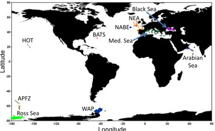
We collected data from various projects (Table S1) that incor-porated ship-based measurements of NPP profiles covering ten regions (Fig. 1) and spanning multiple time-periods be-tween 1984–2007 (Table 1). Although each dataset included NPP, the over-arching goals and purposes for each of these field studies were diverse and were not optimized in their sampling design to assess ocean color models. However, in situ measurements of marine NPP are not common thus we had to use a diverse group of datasets. All 1156 NPP mea-surements were based on the14_{C tracer method; incubation}

times and type (in situ or on-deck) were dependent upon time of year and region, respectively (Table 1). Each station’s NPP profile was measured to the 1% light-level at various depth intervals. We extracted each station’s NPP datum at every depth of measurement and used trapezoid integration to provide daily NPP (mg C m−2day−1) to the greatest isol-ume measured (1% light-level). Because 24-h incubations are more accurate measurements of NPP (Campbell et al., 2002), we adjusted NPP measurements that were based on

(3)

Latitude Longitude !"#$ %&'($ )*++$,-.$ /%&$ 0%#,$ %1.23.4$ ,-.$ 5-67$,-.$ 8%09$ 89%$ 0:.;<$,-.$

Fig. 1. Sample locations of the 1156 NPP measurements among 10

regions. Some of these locations were sampled multiple times (i.e. BATS and HOT).

incubation time shorter than 24 h. These regions were the Bermuda Atlantic Time-series Study (BATS) and the Hawaii Ocean Time-series (HOT) where primary productivity was measured using 12–16 h incubations (Table 1). At BATS, in-cubations were performed using both light and dark bottles, whereas at HOT, dark bottles have not been used since 2000. Therefore, we calculated NPP in the following manner: for the BATS data, we used the mean light values of productiv-ity and subtracted the dark values to remove the carbon pro-duced by non-photoautotrophs. For the HOT data, we cal-culated the average proportion of dark to light bottle values from 1989 to 2000 and then used this proportion to calculate NPP for all light bottle samples from 2000 onwards.

Ocean color models require specific input data to estimate NPP; the suite of input data is dependent upon model type although all ocean color models require surface measure-ments of chlorophyll-a (Chl-a) (Table 2). For each station, we used in situ surface fluorometric Chl-a and in situ sea surface temperature (SST) from the programs listed in Ta-ble 1 (surface= 0–5 m). Reanalysis estimates of shortwave radiation were obtained from the National Centers for En-vironmental Prediction (http://www.cdc.noaa.gov) and trans-formed to photosynthetically active radiation (PAR; Ein-steins m−2d−1) using a conversion factor of 0.43 (Olofs-son et al., 2007). Mixed-layer depths (MLD) were derived either from in situ measurements using the surface offset method (!σ= 0.125 kg m−3)(Levitus, 1982) or from model results (WAP= Dinniman and Klinck, 2004; BATS and NEA= Doney, 1996; Doney et al., 2007; Black Sea = Kara et al., 2005; Mediterranean Sea= D’Ortenzio et al., 2005).

Depth data for each station were extracted from the British Oceanographic Data Centre (http://www.bodc.ac.uk/ data/online delivery/gebco) using one arc-minute grid data from the gridded bathymetric data sets. The complete dataset used for this analysis can be found in the online Supplement (Supplement file S1).

2.2 Models

Output from a total of 21 satellite-based ocean color models were contributed to this study (Table 2). Model complex-ity ranged from the relatively simple depth-integrated and/or wavelength-integrated models to the more complex depth-resolved and wavelength-depth-resolved models. Specific details for each of the 21 models are given in Appendix A of the Supplement. Model participants were provided with input fields (Chl-a, SST, PAR, MLD, latitude/longitude, date, and day length) and returned estimates of NPP integrated to the base of the euphotic zone (1% light-level). Although skill comparison results for the carbon-based models (Behrenfeld et al., 2005; Westberry et al., 2008) appear in Friedrichs et al. (2009) and Saba et al. (2010), these approaches are not cluded in the analyses presented here. One of the primary in-puts for the carbon-based model is particulate backscattering, which is not included in the dataset described in Sect. 2.1, and which severely handicaps these models for the purposes of this type of evaluation. Satellite surrogates for particulate backscatter are available for use with some of the dataset as-sembled here, but are not available for the subset of data prior to the modern ocean color satellite era (prior to 1997).

2.3 Model performance

To assess overall model performance in terms of both bias and variability in a single statistic, we used the root mean square difference (RMSD) calculated for each model’s N es-timates of NPP: RMSD = ! 1 N N " i=1 !(i)2 #1/2 (1)

where model-data misfit in log10space !(i) is defined as:

!(i) = log(NPPm(i))−log(NPPd(i)) (2)

and where NPPm(i)is modeled NPP and NPPd(i)represents

in situ data for each sample i. The RMSD statistic assesses model skill such that models with lower values have higher skill. The use of log normalized RMSD to assess overall model performance is consistent with prior PPARR studies (Campbell et al., 2002; Carr et al., 2006; Friedrichs et al., 2009; Saba et al., 2010). To assess model skill more specif-ically (whether a model over- or underestimated NPP), we calculated each model’s bias (B) for each region where:

B= log(NPPm)−log(NPPd) (3)

We determined if certain model types or individual models had significantly higher skill than others (based on RMSD) by applying an ANOVA method with a 95% confidence in-terval.

Model performance was also illustrated using Target dia-grams (Jolliff et al., 2009). These diadia-grams break down the RMSD such that:

(4)

Table 1. Description of each region and study from which NPP measurements were recorded.

General region Program Ecosystem type N Sampling time range Spatial NPP method (incubation,

coverage tracer, incubation time)

Northwest Atlantic Ocean: BATS∗ Subtropical – Gyre 197 Dec 1988 to Dec 2003 Single in situ,14C, 12–16 h

Sargasso Sea station

Northeast Atlantic Ocean NABE Temperate – 12 Apr 1989 to May 1989 Multiple in situ,14C, 24 h

Convergence Zone stations

Northeast Atlantic Ocean NEA (OMEX I, II), Temperate – 52 Jul 1993 to Jul 1999 Multiple on deck,14C, 24 h

SeaMARC Convergence Zone stations

Black Sea NATO SfP ODBMS Temperate 43 Jan 1992 to Apr 1999 Multiple on deck,14_{C, 24 h}

Anoxic Basin stations

Mediterranean Sea DYFAMED, FRONTS, Temperate Basin 86 Feb 1990 to Sep 2007 Multiple on deck,14C, 24 h

HIVERN, PROSOPE, stations

VARIMED, ZSN-GN

Arabian Sea Arabian Sea Tropical – Monsoonal 42 Jan 1995 to Dec 1995 Multiple in situ,14C, 24 h

(Process Study) stations

North Pacific Ocean HOT Subtropical – Gyre 139 Jul 1989 to Dec 2005 Single in situ,14_{C, 12–16 h}

station

Southern Ocean Ross Sea Polar – Polynya 133 Oct 1996 to Dec 2006 Multiple on deck,14C, 24 h

(AESOPS, CORSACS) stations

Southern Ocean WAP (LTER-PAL) Polar – 440 Jan 1998 to Jan 2005 Multiple on deck,14C, 24 h

Continental Shelf stations

Southern Ocean APFZ (AESOPS) Polar – 12 Dec 1997 Multiple on deck,14C, 24 h

Convergence Zone stations

∗Program descriptions are listed in Table S1 of the Supplement.

Table 2. Contributed satellite-based ocean color primary productivity models. Specific details for each model are described in Appendix A

of the Supplement.

Model # Contributer Type Input variables used: Reference

Chl-a SST PAR MLD

1 Saba DI, WI x Eppley et al. (1985)

2 Saba DI, WI x x x x Howard and Yoder (1997)

3 Saba DI, WI x x x Carr (2002)

4 Dowell DI, WI x x x x Dowell, unpublished data

5 Scardi DI, WI x x x x Scardi (2001)

6 Ciotti DI, WI x x x Morel and Maritorena (2001)

7 Kameda; Ishizaka DI, WI x x x Kameda and Ishizaka (2005)

8 Westberry; Behrenfeld DI, WI x x x Behrenfeld and Falkowski (1997)

9 Westberry; Behrenfeld DI, WI x x x Behrenfeld and Falkowski (1997); Eppley (1972)

10 Tang DI, WI x x x Tang et al. (2008); Behrenfeld and Falkowski (1997)

11 Tang DI, WI x x x Tang et al. (2008)

12 Armstrong DR, WI x x x Armstrong (2006)

13 Armstrong DR, WI x x x Armstrong (2006); Eppley (1972)

14 Asanuma DR, WI x x x Asanuma et al. (2006)

15 Marra; O’Reilly; Hyde DR, WI x x x Marra et al. (2003)

16 Antoine; Morel DR, WR x x x x Antoine and Morel (1996)

17 Uitz DR, WR x x x Uitz et al. (2008)

18 M´elin; Hoepffner DR, WR x x M´elin and Hoepffner (2011)

19 Smyth DR, WR x x x Smyth et al. (2005)

20 Waters DR, WR x x x x Ondrusek et al. (2001)

21 Waters DR, WR x x x Ondrusek et al. (2001)

(5)

where unbiased RMSD squared (uRMSD2₎_{is defined as:} uRMSD2=1 N N " i=1 $

(logNPPm(i)−logNPPm)

−(logNPPd(i)−logNPPd)%2 (5)

Target diagrams show multiple statistics on a single plot: bias on the y-axis, and the signed unbiased RMSD (uRMSD) on the x-axis, where:

signed uRMSD=(uRMSD) sign(σm−σd) (6)

and σm= standard deviation of log NPPmand σd= standard

deviation of log NPPd. The Target diagram thus enables one

to easily visualize whether a model over- or under-estimates the mean and variability of NPP. By normalizing the bias and uRMSD by σdand plotting a circle with radius equal to one,

the Target diagrams also illustrate whether models are per-forming better than the mean of the observations (Jolliff et al., 2009). Models that perform better than the mean of the observations are defined to have a Model Efficiency (ME) greater than zero (Stow et al., 2009):

ME=

N

&

i=1

'

logNPPd(i)−logNPPd(2−

N

&

i=1{logNPP

m(i)−logNPPd(i)}2

N

&

i=1

'

logNPPd(i)−logNPPd(

2 (7)

The ME is located inside the reference circle on the Target diagrams. A model with ME < 0 is typically of limited use, because the data mean provides a better fit to the observa-tions than the model predicobserva-tions. In the NPP comparisons presented here, models produce the lowest RMSD for the re-gional data sets characterized by the least variability, yet at the same time these models can have ME < 0. When data sets have low variability, it is difficult for models to do better than the mean of the observations. To be consistent with pre-vious PPARR results, we typically equate higher model skill with lower RMSD, yet we also discuss ME as a secondary indicator of model skill.

Finally, to determine the effect of various station param-eters on the NPP model estimates, for every NPP measure-ment the Pearson’s correlation coefficient was calculated be-tween model-data misfit (!(i)) and each of the following parameters: Chl-a, SST, PAR, MLD, NPP, absolute latitude (i.e. distance from the equator in degrees), and depth.

2.4 Uncertainty analysis

When comparing ocean color model estimates of NPP, it is important to consider uncertainty in the input fields and the NPP data, both of which can affect the assessment of a model’s ability to accurately estimate NPP (Friedrichs et al., 2009). For each measurement of NPP, we as-sumed an uncertainty in the measurement such that val-ues less than or equal to 50 mg C m−2day−1 were sub-ject to a ±50% error, while values greater than or equal

Table 3. Uncertainties in each input variable at each region based

on differences between satellite, modeled, and in situ data sources. Ocean color models were provided with 81 perturbations of input data for each NPP measurement based on these region-specific un-certainties.

Region Chl-a± SST± PAR± MLD±

BATS 35% 1◦C 20% 40% NABE 50% 1◦C 20% 40% NEA 50% 1◦C 20% 20% Black Sea 50% 1◦C 20% 40% Med. Sea 65% 1◦C 20% 40% Arabian Sea 50% 1◦C 20% 40% HOT 35% 1◦C 20% 40% Ross Sea 65% 1◦C 20% 60% WAP 65% 1◦C 20% 60% APFZ 65% 1◦C 20% 40%

to 2000 mg C m−2day−1 were subject to a ±20% error (W. Smith, unpublished data). Therefore, error in values between 50 and 2000 mg C m−2day−1ranged from 50% to 20% respectively and were calculated using a linear function of log(NPP).

Ocean color models use satellite-derived input data, thus it is important to understand how their estimates of NPP can be affected by error in these data. For that purpose, we compared each station’s in situ Chl-a and modeled PAR to 8-day, level-3 SeaWiFS 9 km data from the NASA Ocean Color Website (http://oceancolor.gsfc.nasa.gov). SeaWiFS measurements of Chl-a and PAR were averaged for the 3×3 grid point window (27×27 km) that encompassed each NPP measurement location. This was done for each 8-day Sea-WiFS image that contained the respective date of each mea-surement. Comparing in situ Chl-a to 8-day Level 3 Sea-WiFS data was not ideal but it was a compromise solu-tion to get a maximum uncertainty estimate for each re-gion. However, ocean color models typically use Level-3, monthly or 8-day, satellite-derived Chl-a and thus we were able to get an idea of RMSD sensitivity to in situ ver-sus satellite-derived NPP estimates. For SST, we used an error of±1◦_{C, which was found to be a conservative}

er-ror between in situ and satellite-derived data (Friedrichs et al., 2009) and thus represented a maximum possible un-certainty. We compared MLD to the Thermal Ocean Pre-diction Model (TOPS) (http://www.science.oregonstate.edu/ ocean.productivity/mld.html), which is based on the Navy Coupled Data Assimilation. We extracted 8-day TOPS MLD data for each station using the same method for SeaWiFS Chl-a and PAR. There are no SeaWiFS or TOPS data prior to September of 1997 thus we only compared NPP measure-ments that were collected since 1997 to calculate uncertainty.

(6)

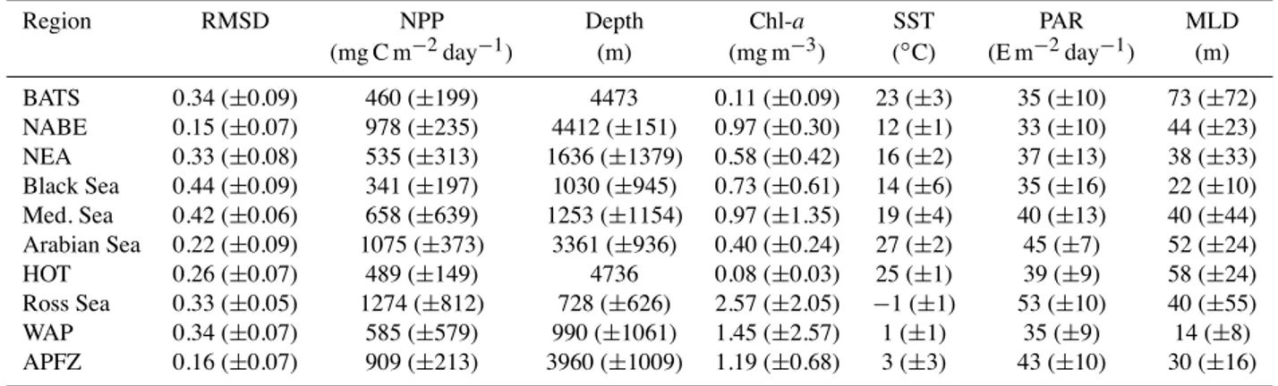
Table 4. Mean RMSD (model skill), depth, in situ NPP, and input data (± standard deviation) for each of the ten regions.

Region RMSD NPP Depth Chl-a SST PAR MLD

(mg C m−2day−1) (m) (mg m−3) (◦C) (E m−2day−1) (m) BATS 0.34 (±0.09) 460 (±199) 4473 0.11 (±0.09) 23 (±3) 35 (±10) 73 (±72) NABE 0.15 (±0.07) 978 (±235) 4412 (±151) 0.97 (±0.30) 12 (±1) 33 (±10) 44 (±23) NEA 0.33 (±0.08) 535 (±313) 1636 (±1379) 0.58 (±0.42) 16 (±2) 37 (±13) 38 (±33) Black Sea 0.44 (±0.09) 341 (±197) 1030 (±945) 0.73 (±0.61) 14 (±6) 35 (±16) 22 (±10) Med. Sea 0.42 (±0.06) 658 (±639) 1253 (±1154) 0.97 (±1.35) 19 (±4) 40 (±13) 40 (±44) Arabian Sea 0.22 (±0.09) 1075 (±373) 3361 (±936) 0.40 (±0.24) 27 (±2) 45 (±7) 52 (±24) HOT 0.26 (±0.07) 489 (±149) 4736 0.08 (±0.03) 25 (±1) 39 (±9) 58 (±24) Ross Sea 0.33 (±0.05) 1274 (±812) 728 (±626) 2.57 (±2.05) −1 (±1) 53 (±10) 40 (±55) WAP 0.34 (±0.07) 585 (±579) 990 (±1061) 1.45 (±2.57) 1 (±1) 35 (±9) 14 (±8) APFZ 0.16 (±0.07) 909 (±213) 3960 (±1009) 1.19 (±0.68) 3 (±3) 43 (±10) 30 (±16)

Uncertainties in each input variable were calculated for each region (Table 3). Each of the four input variables can have three possible values for each NPP measurement (orig-inal value, orig(orig-inal value + uncertainty, orig(orig-inal value – un-certainty). Similarly, each NPP measurement could also have three values (the original value and the observed± uncer-tainty). Therefore, for each NPP measurement (N= 1156) there are 81 perturbations of input data and three possi-ble values of NPP. Model participants were provided with 1156× 81 perturbations of input data and the uncertainty analysis was conducted as follows: for each NPP measure-ment, we examined the 81 perturbations and selected the perturbation that produced the lowest RMSD using (a) un-certainty in individual input variables, (b) unun-certainty in all input variables, (c) uncertainty in observed NPP, and (d) un-certainty in all input variables and in observed NPP.

3 Results

3.1 Observed data

Measurements of NPP ranged from as low as 18 mg C m−2day−1 in the Ross Sea to as high as 5038 mg C m−2day−1 in the West Antarctic Peninsula (WAP). The region with the highest mean NPP was the Ross Sea (1274 mg C m−2day−1)while the region with the lowest mean NPP was the Black Sea (341 mg C m−2day−1)

(Table 4). The region with the highest variability in NPP was the Mediterranean Sea while the North Atlantic Bloom Experiment (NABE) and the Antarctic Polar Frontal Zone (APFZ) had the lowest variability (Table 4).

Data ranges among the input variables (Table 4) were as follows: Chl-a from 0.005 mg m−3 (BATS) to 23 mg m−3 (WAP); SST from−2◦C (Ross Sea) to 29◦C (Arabian Sea); PAR from 11 E m−2day−1 (Northeast Atlantic, NEA) to 70 E m−2day−1(Ross Sea); and MLD from 2 m (WAP) to 484 m (Ross Sea). 0.0 0.1 0.2 0.3 0.4 0.5 0.6

BATS NABE NEA Black

Sea MED Arabian Sea HOT Ross Sea WAP APFZ 0.0 0.1 0.2 0.3 0.4 0.5 0.6

BATS NABE NEA Black

Sea MED Arabian Sea HOT Ross Sea WAP APFZ RMSD Region

Fig. 2. Average RMSD for all 21 models at each region. Lower

val-ues of RMSD are equivalent to higher model skill. Green error bars

are 2× standard error. Red bars represent the maximum reduction

in RMSD (increase in model skill) when the uncertainty in both the input variables and in situ NPP measurements are considered.

3.2 Region-specific model performance 3.2.1 Total RMSD

In terms of the average skill of the 21 ocean color mod-els, RMSD was not consistent (P < 0.0001) at each of the ten regions (Table 4; Fig. 2). Average ocean color model skill was significantly lower (P < 0.0001) in the Black and Mediterranean Seas (mean RMSD= 0.44 and 0.42, respec-tively) when compared to the other eight regions (0.27) (Ta-ble 4; Fig. 2). Among the other eight regions, there were significant differences between specific groups. The hierar-chy of average model skill (highest to lowest; P < 0.005) for groups of regions that had statistically significant differences in RMSD is as follows: the NABE and APFZ (0.15); the Ara-bian Sea and HOT (0.24); BATS, NEA, the Ross Sea, and

(7)

0.0 0.1 0.2 0.3 0.4 0.5 0.6 1 2 3 4 5 6 7 8 9 10 11 12 13 14 15 16 17 18 19 20 21 0.0 0.1 0.2 0.3 0.4 0.5 0.6 1 2 3 4 5 6 7 8 9 10 11 12 13 14 15 16 17 18 19 20 21 Best Models 0.0 0.1 0.2 0.3 0.4 0.5 0.6 1 2 3 4 5 6 7 8 9 10 11 12 13 14 15 16 17 18 19 20 21 0.0 0.1 0.2 0.3 0.4 0.5 0.6 1 2 3 4 5 6 7 8 9 10 11 12 13 14 15 16 17 18 19 20 21 0.0 0.1 0.2 0.3 0.4 0.5 0.6 1 2 3 4 5 6 7 8 9 10 11 12 13 14 15 16 17 18 19 20 21 0.0 0.1 0.2 0.3 0.4 0.5 0.6 1 2 3 4 5 6 7 8 9 10 11 12 13 14 15 16 17 18 19 20 21 0.0 0.1 0.2 0.3 0.4 0.5 0.6 1 2 3 4 5 6 7 8 9 10 11 12 13 14 15 16 17 18 19 20 21 0.0 0.1 0.2 0.3 0.4 0.5 0.6 1 2 3 4 5 6 7 8 9 10 11 12 13 14 15 16 17 18 19 20 21 0.0 0.1 0.2 0.3 0.4 0.5 0.6 1 2 3 4 5 6 7 8 9 10 11 12 13 14 15 16 17 18 19 20 21 0.0 0.1 0.2 0.3 0.4 0.5 0.6 1 2 3 4 5 6 7 8 9 10 11 12 13 14 15 16 17 18 19 20 21 RMSD Arabian Sea Ross Sea Med. Sea APFZ HOT WAP BATS NABE

NEA Black Sea

Model

Fig. 3. Model skill (RMSD) for each model at each region. Solid

black line is the RMSD when using the mean of the observed data. Models that have a RMSD below the solid black line have a Model Efficiency >0 thus they estimate NPP more accurately than using the mean of the observed data.

WAP (0.33); and finally the Black and Mediterranean Seas (0.43) (Table 4; Fig. 2). Within each of these four groups of regions, model skill was not significantly different.

In terms of individual model skill, certain models per-formed better than others in specific regions (Fig. 3). Model 16 (Antoine and Morel, 1996) was among the best models (in terms of lowest RMSD) in eight of ten regions and had ME > 0 in three regions (Fig. 3). Models 9 (Behren-feld and Falkowski, 1997; Eppley, 1972) and 12 (Armstrong, 2006) were among the best models in seven of ten regions (in terms of lowest RMSD) and had ME > 0 in five regions (Fig. 3). Model 7 (Kameda and Ishizaka, 2005) was among the best models in six of ten regions (Fig. 3) and had ME > 0 in four regions. -2.0 -1.0 0.0 1.0 2.0 -2.0 -1.0 0.0 1.0 2.0 Bias uRMSD* Bias* -2.0 -1.0 0.0 1.0 2.0 -2.0 -1.0 0.0 1.0 2.0 Bias uRMSD* Bias* DIWI DRWR -2.0 -1.0 0.0 1.0 2.0 -2.0 -1.0 0.0 1.0 2.0 Bias uRMSD* Bias* DRWI -4.0 -3.0 -2.0 -1.0 0.0 1.0 2.0 3.0 4.0 -4.0 -3.0 -2.0 -1.0 0.0 1.0 2.0 3.0 4.0 BATS NABE NEA Black Sea MED Arabian Sea HOT Ross Sea WAP APFZ Bias uRMSD* Bias*

Fig. 4. Target diagrams representing average model skill at each

region for DIWIs (11 models), DRWIs (4 models), and DRWRs (6

models). Bias∗ and uRMSD∗ are normalized such that Bias and

uRMSD are divided by the standard deviation of in situ NPP data

(σd) at each region. The solid circle is the normalized standard

deviation of the in situ NPP data at each region. Symbols falling within the circle indicate that models estimate NPP more accurately than using the mean of the observed data (Model Efficiency >0) at each region. Red symbols are the pelagic regions and blue symbols are coastal.

The ME statistic was not consistent between regions (Figs. 3 and 4). In the Ross Sea, all models estimated NPP more accurately than using the mean of the observed data (ME > 0) whereas none of the models did better than the observed data mean in BATS and the Black Sea (ME < 0) (Figs. 3 and 4).

3.2.2 Bias and variance

Target diagrams were used to illustrate the ability of ocean color models to estimate NPP more accurately than using the observed mean for each region (values in Table 4) such that symbols within the solid circle were successful (ME > 0) and those lying on the circle or outside were not (ME≤ 0). This ability was a function of both the type of ocean color model and the region (Fig. 4). The depth/wavelength in-tegrated models fell within the solid circle for the Ara-bian and Ross Seas, WAP, and the APFZ; the depth re-solved/wavelength integrated models for the Mediterranean and Ross Seas, and WAP; and the depth/wavelength resolved models for NABE, the Mediterranean, Arabian and Ross Seas, and APFZ (Fig. 4).

In terms of average bias, the models either overestimated the observed mean NPP or estimated it with no bias in the

(8)

NPP (36%) All Input (50%) Chl-a (35%) PAR (11%) SST (6%) MLD (3%) Region BATS Parameter NPP+Input (72%) Percent reduction in RMSD 50 60 70 80 90 100 0 10 20 30 40

NABE NEA Black Sea Med. Sea Arabian Sea HOT Ross Sea WAP APFZ

Fig. 5. Reduction in RMSD at each region based on uncertainties

in individual input parameters, all input parameters, NPP measure-ments, and both the input parameters and NPP measurements. Val-ues in parentheses are mean reductions in RMSD across all regions.

five shallowest regions (NEA, Black Sea, Mediterranean Sea, Ross Sea, WAP; Fig. 4). Conversely, the models all underes-timated the observed mean NPP at BATS, the Arabian Sea, and HOT (Fig. 4). However, at NABE and APFZ, the sign of bias depended on whether depth and wavelength were re-solved.

In contrast to the bias results discussed above, the abil-ity of the models to reproduce NPP variabilabil-ity was not a function of depth, but was more a function of model type. The depth/wavelength resolved models underestimated NPP variability in all regions except the APFZ. On average, the three of types models overestimated the variance at the APFZ while underestimating the variance in the Black and Mediter-ranean Seas, HOT, Ross Sea, and WAP (Fig. 4). In the other four regions, the sign of uRMSD depended on whether depth and wavelength were resolved. Finally, total RMSD was not a function of whether or not depth and wavelength were re-solved (Fig. 4).

3.2.3 Uncertainty analysis

The range of uncertainty in NPP measurements across all regions (N = 1156) was from ±11 to ±629 mg C m−2day−1 with an average uncertainty of ±31% (±175 mg C m−2_day−1₎_{. Average uncertainty for Chl-a was}

±60% (±0.54 mg m−3₎_{, MLD}_{± 41% (±17 m), PAR ± 20%}

(±8 E m−2_day−1₎_{, and SST}_{± 7% (±1}◦_{C). When the}

un-certainty in both the input variables and NPP measurements were considered at each of the ten regions, average RMSD significantly decreased by nearly 72% (P < 0.0005) in ev-ery region (Figs. 2 and 5). Uncertainties in Chl-a and NPP measurements accounted for the largest individual-based re-ductions in RMSD across all regions (35% and 36%, respec-tively) (Fig. 5). The uncertainty in NPP measurements had the smallest influence (23%) on RMSD in the Mediterranean

0.0 0.1 0.2 0.3 0.4 0.5 1 2 3 4 5 6 7 8 9 10 11 12 13 14 15 16 17 18 19 20 21 DIWI DRWI DRWR RMSD Model

Fig. 6. Average RMSD for each model across all regions. Error

bars are 2× standard error.

Sea but had the largest influence (46% to 60%) for NABE, HOT, and APFZ (Fig. 5). Uncertainty in Chl-a had the small-est influence (21%) on RMSD at BATS but had the largsmall-est influence (44% and 53%) at the APFZ and NABE (Fig. 5). Among uncertainties in the other individual input variables PAR, MLD, and SST, the average reduction in RMSD was only 6% (Fig. 5).

3.3 Model performance across all regions 3.3.1 Individual model skill

When individual model skill was averaged over all ten re-gions, there were no significant differences in mean RMSD for the 21 ocean color models (Fig. 6). Average RMSD for the 21 models was 0.30 (±0.02 (2 × standard error)). There were also no significant differences between the three types of ocean color models (Fig. 6): a. Average RMSD for DIWI, DRWI, and DRWR models was 0.30 (±0.02), 0.30 (±0.02), and 0.28 (±0.04), respectively.

3.3.2 Relationship between model-data misfit and station parameters

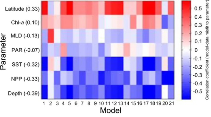
The behavior of these models was investigated further by ex-amining the correlation of model-data misfit to various pa-rameters across all regions (Fig. 7). The highest tion coefficient was found for station depth (mean correla-tion=−0.39) followed by observed NPP (−0.33), latitude (0.33), and SST (−0.32) (Figs. 7 and 8). The highest corre-lation between model-data misfit and station depth was for Model 17 (−0.65) and the lowest was for Model 20 (0.01) (Fig. 7). The lowest correlation between model-data misfit and observed NPP was for Model 2 (−0.05) while Model 20 had the highest (−0.77) (Fig. 7). For both latitude and SST, Model 3 had the lowest correlation (0.04 and −0.04) while Model 17 had the highest (0.73 and−0.72) (Fig. 7).

(9)

Chl-a (0.10) MLD (-0.13) PAR (-0.07) SST (-0.32) NPP (-0.33) Depth (-0.39) Model 1 2 3 4 5 6 7 8 9 10 11 12 13 14 15 16 17 18 19 20 21 Parameter Latitude (0.33)

Correlation coefficient (model-data misfit to parameter)

0 0.1 0.2 0.3 0.4 0.5 -0.5 -0.4 -0.3 -0.2 -0.1

Fig. 7. Correlation between model-data misfit (!(i)) and various

parameters across all regions for individual models. Absolute val-ues of latitude were used. Valval-ues in parentheses are average corre-lation coefficients for each parameter across all models.

Although Chl-a, MLD, and PAR did not produce correla-tions to|model-data misfit| that were higher than |0.30| for groups of models, some individual models did stand out for Chl-a (Models 17 and 20) and MLD (Model 2) (Fig. 7). For PAR, no individual model had a correlation that was higher than|0.30| (Fig. 7).

The general relationship between model-data misfit and station depth was such that the models overestimated NPP at shallow stations, underestimated NPP at deep stations, and had the greatest skill at stations in 2500–3500 m water depth (Fig. 8). The models generally produced a smaller range of NPP values than observed: they overestimated NPP when NPP was low and underestimated NPP when NPP was high, with optimal model-data fit at NPP∼900– 1000 mg C m−2day−1(Fig. 8). For SST, the models tended to overestimate NPP at SST below 5◦C, overestimate NPP at SST between 5 and 15◦C, and underestimate NPP at SST above 20◦C (Fig. 8). The correlation between model-data misfit and latitude (Fig. 7) was likely driven by the high cor-relation between SST and latitude (−0.96).

3.3.3 Model performance as a function of water column depth

In terms of average RMSD from the 21 models, skill was sig-nificantly higher (P < 0.01) at stations with depths greater than 250 m (Fig. 9). When the uncertainty of both the input variables and NPP measurements were considered, model skill significantly increased across the three depth ranges but the relationship between them was unchanged. When only the stations shallower than 250 m were considered, those

<125 m had significantly lower skill (mean RMSD= 0.44± 0.05 standard deviation) than those between 125 and 250 m (0.39±0.05). However, stations between 125 and 250 m had significantly lower skill than those greater than 250 m.

In terms of the performance of individual models within these depth intervals (Fig. 10), only Model 7 (Kameda and

Ishizaka, 2005) had no substantial change in skill (relative to the change in skill for the other models) as a function of station depth (Fig. 10a). Within each of the three depth ranges, model skill (as a group) was a function of either SST (Fig. 10b) or surface Chl-a but not both (Fig. 10c). For stations with depths between 0–250 m, the models had sta-tistically higher skill (P < 0.0001) at SST > 20◦C than at SST < 20◦C (Fig. 10b) but had no difference in skill at the three ranges of surface Chl-a (Fig. 10c). For depths between 250–750 m, model skill was highest at SST > 20◦C, interme-diate at SST < 10◦C, and lowest at SST between 10–20◦C (P < 0.0001; Fig. 10b) but no difference in model skill at the three ranges of surface Chl-a (Fig. 10c). For depths greater than 750 m, there was no difference in model skill at the three ranges of SST (Fig. 10b) although model skill was highest (P < 0.005) at surface Chl-a concentrations <0.5 mg m−3 and >1.0 mg m−3(Fig. 10c). Although these statistical com-parisons (ANOVA) were based on groups of models, a few individual models did not have similar statistics. For exam-ple, within the 250–750 m depth range, Models 2 (Howard and Yoder, 1997) and 21 (Ondrusek et al., 2001) had a wide range of skill at the three surface Chl-a ranges whereas all of the models as a group did not (Fig. 10c).

4 Discussion

4.1 Region-specific model performance

The average skill of the ocean color models assessed in this study varied substantially from region to region. Although the sample size of in situ NPP measurements and number of ocean color models tested were much higher than in the pre-vious multi-regional PPARR study (Campbell et al., 2002), our results were similar in that model skill was a strong func-tion of region. Although we cannot compare results in most cases because of sample size differences, the NABE NPP measurements compared in this study were identical to those used in Campbell et al. (2002) and thus in this case we can compare ocean color model skill between the two studies. The average RMSD among 12 ocean color models at NABE from Campbell et al. (2002) was 0.31 whereas the average RMSD from our study was 0.14. Our results suggest that the increase in skill is due to either or both: (1) improvements to particular algorithms that were used here and in Campbell et al. (2002); (2) the higher sample size of better-performing models since the Campbell et al. (2002) study, at least in the NABE region where ocean color model skill increased by nearly 50%.

Ocean color models were most challenged in the Black and Mediterranean Seas; these two regions also had the largest proportion of station depths that were less than 250 m (Black Sea 44%; Mediterranean Sea 36%) where average model skill was lowest. These results suggest that the shal-low depths of the Black and Mediterranean Seas resulted in

(10)

-1.5 -1.0 -0.5 0.0 0.5 1.0 1.5 0 5 10 15 20 25 30 -1.5 -1.0 -0.5 0.0 0.5 1.0 1.5 0 500 1000 1500 2000 2500 3000 3500 -1.5 -1.0 -0.5 0.0 0.5 1.0 1.5 0 10 20 30 40 50 60 70 80 90

Model-data misfit [

log(

m

)-log(

d)]

Depth (m)

Absolute latitude (degrees)

NPP (mg C m

-2

_day

-1

₎

_{Chl-a (mg m}

-3

₎

SST (

o

_C)

-1.5 -1.0 -0.5 0.0 0.5 1.0 1.5 0 500 1000 1500 2000 2500 3000 3500 4000 4500 5000 0-250 m 250-750 m > 750 m -1.5 -1.0 -0.5 0.0 0.5 1.0 1.5 0 5 10 15 20 25

Fig. 8. Relationship between model-data misfit (!(i)) and five parameters (depth, latitude, NPP, Chl-a, and SST) across all regions. Each

point is color-coded by depth. Points above the horizontal dashed line are NPP overestimates while those below are underestimates. Trend lines are shown for correlation coefficients greater than 0.30. Note the SST relationship is based on polynomial regression.

the poor skill of ocean color models, especially given the high sensitivity of model-data misfit to station depth (see Sect. 4.4).

There was no difference in mean RMSD between the NABE and APFZ, the two regions where models had the highest skill. These regions shared multiple characteristics that may have led to the high skill of the models: they were among the deepest stations in the study, mean NPP was be-tween 900–1000 mg C m−2day−1, and most importantly the NPP measurements were obtained over one month of a single year that sampled the spring phytoplankton bloom, and were thus characterized by low variability. If a longer temporal coverage of the NABE and APFZ were available, the sea-sonal variability of NPP would have been stronger, possibly further challenging the models to estimate NPP. The NABE and APFZ had the lowest observed variability in NPP (±24%

standard deviation of the mean) followed by the Arabian Sea and HOT (±33%). The Arabian Sea and HOT regions fol-lowed the NABE and APFZ in the hierarchy of model skill thus one might suspect that model skill is driven by the level of NPP variability in the region. However, we found this not to be the case among the remaining regions (BATS, NEA, Ross Sea, and WAP) where models performed equally and NPP variability was not consistent. There may be a thresh-old of NPP variability (<35%) that affects model skill, how-ever, the four regions where models had the highest skill were also among the deepest stations. Therefore, the high perfor-mance of the models at the NABE, APFZ, Arabian Sea, and HOT may be driven by a combination of low NPP variability (<35%), deep station depth (>2000 m), and moderate NPP (900–1000 mg C m−2day−1).

(11)

0.0 0.1 0.2 0.3 0.4 0.5 0.6 0-250 m 250-750 m 750+ m 0.0 0.1 0.2 0.3 0.4 0.5 0.6 0-250 m 250-750 m 750+ m 0.0 0.1 0.2 0.3 0.4 0.5 0.6 0-250 m 250-750 m 750+ m 0.0 0.1 0.2 0.3 0.4 0.5 0.6 0-250 m 250-750 m 750+ m RMSD Depth range

Fig. 9. Average RMSD for all 21 models at each depth range. Green

error bars are 2× standard error. Red bars represent the maximum

reduction in RMSD when the uncertainty in both the input variables and in situ NPP measurements are considered.

Of the eight regions investigated by Campbell et al. (2002), ocean color models had the lowest skill in those characterized by High-Nitrate Low-Chlorophyll (HNLC) re-gions, i.e. the equatorial Pacific and the Southern Ocean. In their comparison of globally modeled NPP using satellite-derived input variables, Carr et al. (2006) found that modeled NPP significantly diverged in HNLC regions.

Using the results from the present study along with a re-cent PPARR study that compared ocean color model NPP es-timates to in situ data in the tropical Pacific where 60% of the stations were in HNLC waters (Friedrichs et al., 2009), we can further assess model estimates in HNLC regions. Mean RMSD of 21 ocean color models tested in the tropical Pa-cific was 0.29 (Friedrichs et al., 2009), which is similar in skill to the Arabian Sea (0.22) and HOT (0.26) where the 21 models tested here performed relatively well (skill was only higher in the NABE and APFZ regions). The average RMSD from the three Southern Ocean regions tested here (Ross Sea, WAP, and APFZ) was 0.28. Comparing these regions to the average RMSD of the other four regions in this study (BATS, NEA, the Black Sea, and Mediterranean Sea= 0.38), ocean color models performed better in HNLC regions such as the Southern Ocean and tropical Pacific. Therefore, it appears that the set of ocean color model algorithms tested here and in Friedrichs et al. (2009) may represent an improvement over those used in Campbell et al. (2002), specifically in that the NPP model estimates in HNLC regions are performing just as well if not better than in non-HNLC regions.

Contrary to expectations, the ocean color models tested here were not particularly challenged in extreme conditions of Chl-a and SST. The three Southern Ocean regions had an average SST of 1◦C and a wide range values of Chl-a yet the models had higher skill there than in regions with much warmer SST and average Chl-a concentrations. Our results show agreement with Carr et al. (2006) such that the

rela-(a) Model 1 2 3 4 5 6 7 8 9 10 11 12 13 14 15 16 17 18 19 20 21 1 2 3 4 5 6 7 8 9 10 11 12 13 14 15 16 17 18 19 20 21 1 2 3 4 5 6 7 8 9 10 11 12 13 14 15 16 17 18 19 20 21 _0.55 0.50 0.45 0.40 0.35 0.30 0.25 0.20 RMSD < 10(N = 76) 0-250 m 250-750 m 750+ m 0-250 m 250-750 m 750+ m 0-250 m 250-750 m 750+ m 10-20 (N = 39) > 20 (N = 15) < 10(N = 374) 10-20 (N = 12) > 20 (N = 4) < 10(N = 153) 10-20 (N = 125) > 20 (N = 358) < 0.5(N = 37) 0.5-1.0 (N = 30) > 1.0 (N = 63) < 0.5(N = 80) 0.5-1.0 (N = 100) > 1.0 (N = 210) < 0.5(N = 503) 0.5-1.0 (N = 67) > 1.0 (N = 66) (N = 130) (N = 390) (N = 636) SST ( oC ) Surface Chl -a (mg m -3) (b) Model 1 2 3 4 5 6 7 8 9 10 11 12 13 14 15 16 17 18 19 20 21 1 2 3 4 5 6 7 8 9 10 11 12 13 14 15 16 17 18 19 20 21 1 2 3 4 5 6 7 8 9 10 11 12 13 14 15 16 17 18 19 20 21 _0.55 0.50 0.45 0.40 0.35 0.30 0.25 0.20 RMSD < 10(N = 76) 0-250 m 250-750 m 750+ m 0-250 m 250-750 m 750+ m 0-250 m 250-750 m 750+ m 10-20 (N = 39) > 20 (N = 15) < 10(N = 374) 10-20 (N = 12) > 20 (N = 4) < 10(N = 153) 10-20 (N = 125) > 20 (N = 358) < 0.5(N = 37) 0.5-1.0 (N = 30) > 1.0 (N = 63) < 0.5(N = 80) 0.5-1.0 (N = 100) > 1.0 (N = 210) < 0.5(N = 503) 0.5-1.0 (N = 67) > 1.0 (N = 66) (N = 130) (N = 390) (N = 636) SST ( oC ) Surface Chl -a (mg m -3) Model 1 2 3 4 5 6 7 8 9 10 11 12 13 14 15 16 17 18 19 20 21 1 2 3 4 5 6 7 8 9 10 11 12 13 14 15 16 17 18 19 20 21 1 2 3 4 5 6 7 8 9 10 11 12 13 14 15 16 17 18 19 20 21 _0.55 0.50 0.45 0.40 0.35 0.30 0.25 0.20 RMSD < 10(N = 76) 0-250 m 250-750 m 750+ m 0-250 m 250-750 m 750+ m 0-250 m 250-750 m 750+ m 10-20 (N = 39) > 20 (N = 15) < 10(N = 374) 10-20 (N = 12) > 20 (N = 4) < 10(N = 153) 10-20 (N = 125) > 20 (N = 358) < 0.5(N = 37) 0.5-1.0 (N = 30) > 1.0 (N = 63) < 0.5(N = 80) 0.5-1.0 (N = 100) > 1.0 (N = 210) < 0.5(N = 503) 0.5-1.0 (N = 67) > 1.0 (N = 66) (N = 130) (N = 390) (N = 636) SST ( oC ) Surface Chl -a (mg m -3) (c) Model 1 2 3 4 5 6 7 8 9 10 11 12 13 14 15 16 17 18 19 20 21 1 2 3 4 5 6 7 8 9 10 11 12 13 14 15 16 17 18 19 20 21 1 2 3 4 5 6 7 8 9 10 11 12 13 14 15 16 17 18 19 20 21 _0.55 0.50 0.45 0.40 0.35 0.30 0.25 0.20 RMSD < 10(N = 76) 0-250 m 250-750 m 750+ m 0-250 m 250-750 m 750+ m 0-250 m 250-750 m 750+ m 10-20 (N = 39) > 20 (N = 15) < 10(N = 374) 10-20 (N = 12) > 20 (N = 4) < 10(N = 153) 10-20 (N = 125) > 20 (N = 358) < 0.5(N = 37) 0.5-1.0 (N = 30) > 1.0 (N = 63) < 0.5(N = 80) 0.5-1.0 (N = 100) > 1.0 (N = 210) < 0.5(N = 503) 0.5-1.0 (N = 67) > 1.0 (N = 66) (N = 130) (N = 390) (N = 636) SST ( oC ) Surface Chl -a (mg m -3)

Fig. 10. Model skill (RMSD) for each model at (a) three depth

ranges, (b) three SST ranges at each depth range, and (c) three sur-face Chl-a ranges at each depth range. The station sample size (N ) for each depth range and SST/surface Chl-a range is also listed.

tionship between SST and ocean color model-data misfit is a function of SST range. At SST less than 10◦C, model-data misfit increases with increasing SST while at SST greater than 10◦C, misfit decreases with increasing SST (Fig. 8).

Carr et al. (2006) showed that model estimates of NPP diverged the most in the Southern Ocean, at SST

<10◦C, and at Chl-a concentrations above 1 mg m−3. Our results were similar such that the standard devia-tions among the 21 ocean color model estimates tested here were significantly higher (P < 0.0001) in areas with SST <10◦C (±684 mg C m−2_day−1₎ _{versus SST}

>10◦C (±554 mg C m−2_day−1₎_, _{Chl-a > 1 mg m}−3

(±818 mg C m−2_day−1₎ _versus _{Chl-a < 1 mg m}−3

(±315 mg C m−2_day−1₎_, _{and in the Southern Ocean}

(±692 mg C m−2_day−1₎_{versus areas outside the Southern}

Ocean (±548 mg C m−2_day−1₎_. _{However, if we consider}

individual regions, the highest divergence (P < 0.0001) in model estimates of NPP was in the Mediterranean Sea

(12)

(±1021 mg C m−2_day−1₎_{. Thus in the Mediterranean Sea,}

ocean color models are not only highly challenged in terms of model skill, but also produce the greatest divergence in NPP estimates. It is important to note that model divergence is not always associated with low model skill in terms of model-data misfit or RMSD. For example, RMSD among the 21 models was exactly the same between waters with Chl-a concentrations less than 1 mg m−3(mean RMSD= 0.34) and those above this concentration (mean RMSD= 0.34).

4.2 Model-type performance across all regions

Some of the models tested here were originally developed and tuned for specific regions included in our analysis, and this may explain their higher performance in those regions. Surprisingly, even though certain models performed signifi-cantly better than others in specific regions, the ocean color models generally performed equally well in terms of their average model skill across all ten regions. The simplest em-pirical relationship performed no worse than the most com-plex depth and wavelength resolved models. These results are consistent with Friedrichs et al. (2009) who also reported no effect of ocean color model complexity on model skill.

The most striking result among the models was their per-formance in the Southern Ocean where the extremely low temperatures should have not only affected model skill, but also challenged models that did not use SST as an input vari-able. Surprisingly, there was no statistically significant dif-ference in model skill in the three Southern Ocean regions between models that used SST (17 models; mean RMSD = 0.27 (±0.09)) and those that did not (4 models; mean RMSD= 0.31 (±0.14)). Given the wide SST range of the regions tested here, one may expect models that used SST to outperform those that did not due to the temperature-dependent maximum carbon fixation rate of phytoplankton (Eppley, 1972). Across all regions, models that used SST performed no differently (mean RMSD= 0.30 (±0.12)) than those that did not (mean RMSD= 0.30 (±0.13)); however, model-data misfit among models that did not use SST had a correlation to station SST of−0.58 compared to −0.26 for models that used SST. Therefore, although model-data misfit was correlated to SST for models that did not use SST, it was not high enough to cause a significant difference in skill from the models that used SST.

4.3 Uncertainties in input variables and NPP measurements

When uncertainties in both the input variables and NPP mea-surements were considered, RMSD was reduced by 72%. The largest influence among the input variables was from Chl-a (35% reduction in RMSD). As Friedrichs et al. (2009) found in the tropical Pacific, uncertainties in SST, PAR, and MLD had a relatively small influence on RMSD. The

region-specific uncertainty values used for Chl-a were based on dif-ferences between in situ data and SeaWiFS data to assess the sensitivity of model estimates of NPP to error in satel-lite data. This was an essential analysis given that ocean color models were designed to use satellite-derived input data in order to estimate NPP over large areas and long time-scales; however, we perturbed in situ input data, not satellite-derived data thus the reduction in RMSD from un-certainty in Chl-a would likely not have been as high as 35% if we had based the perturbations on error in the in situ mea-surements. Uncertainties in Chl-a for the PPARR tropical Pacific study based their perturbations on in situ measure-ment error such that the uncertainties ranged from±50% for the minimum concentration (±0.01 mg m−3₎_and_{±15% for}

the maximum concentration (±0.11 mg m−3₎_{resulting in a}

24% increase in ocean color model skill (Friedrichs et al., 2009). Uncertainty in Chl-a for our study averaged±60% (±0.54 mg m−3₎_{across all regions thus explaining why the}

ocean color models here had a greater sensitivity to Chl-a un-certainty. Our goal was to describe the sensitivity of RMSD to differences between in situ and satellite-derived data given that models typically use the latter.

If our estimates of14C measurement uncertainties are cor-rect, then a 36% reduction in RMSD is substantial enough to consider these errors when estimating NPP. Assuming that the change in RMSD based on Chl-a uncertainties is closer to that found in Friedrichs et al. (2009) (24%) as opposed to our values (35%), then our estimate of RMSD difference when uncertainties in both the input variables and NPP mea-surements are considered would be lower than 72% but not likely less than 50%. Therefore, our study confirms the im-portance of both input variable (primarily Chl-a) and NPP uncertainty when using ocean color models to estimate NPP. However, in situ NPP data is not always available for one to consider the error associated with ocean color NPP estimates, therefore, the input variable uncertainty may be a more prac-tical approach to addressing the expected range of estimated NPP. We recommend that ocean color NPP estimates, that are either published or made available online, are accompa-nied with the magnitude of uncertainty in the estimates due to uncertainty in input variables such as SeaWiFS Chl-a and MLD.

4.4 Water column depth and model performance

One of the clearest patterns emanating from this study was the relationship between station depth and average model skill: for stations with water column depths greater than 4000 m, ocean color models typically underestimated NPP whereas they overestimated NPP at depths shallower than 750 m. This positive NPP bias was even greater for depths shallower than 250 m. Interestingly, the relationship be-tween model skill and SST/surface Chl-a was also a func-tion of depth. The models performed significantly better at SST >20◦C at depths less than 750 m whereas SST made

(13)

no difference to model skill at stations deeper than 750 m. Surface Chl-a concentration only affected model skill at the stations deeper than 750 m such that skill was highest at concentrations <0.5 mg m−3 and >1.0 mg m−3. However, one must note that the sample sizes (N ) were not consistent for each depth range and each SST/surface Chl-a range. The RMSD statistic is partially based on N and thus the inconsis-tencies in sample size may have biased our results.

Model skill was significantly lower at the shallow stations and thus the affect of station depth was by far the greatest variable driving model skill. The reason for this relationship is not completely clear. If satellite-derived chlorophyll con-centrations were used in the algorithms, we would have ex-pected the algorithms to perform better in deep Case-1 waters (defined as waters where Chl-a is considered the main driver of optical properties, Morel and Prieur, 1977) because the standard satellite chlorophyll algorithms are known to have difficulty in shallow Case-2 waters where other optically sig-nificant constituents dominate. Here, however, we used in situ chlorophyll concentrations, which are not likely to be associated with greater errors in shallower waters. More-over, surface Chl-a concentration did not affect model skill at depths less than 250 m where Case-2 waters exist.

Most of the models tested here were developed based on in situ data collected in Case-1 waters, a likely explanation for their lower skill in Case-2 waters. A possible reason for the relationship between model bias and water column depth is that the models were overestimating the euphotic zone depth in Case-2 waters and underestimating the eu-photic zone depth in Case-1 waters. The model contributors, however, did not provide their estimates of euphotic zone depth thus we presently have no way of confirming this.

In addition to obtaining estimated euphotic zone depth, another way of possibly resolving this would be to obtain depth-specific output from the depth-resolved models. Our study only required contributors to provide us with integrated NPP. We suggest that future NPP model assessment studies require model contributors to provide detailed output that in-cludes euphotic zone depth estimations in addition to depth-specific NPP estimates from the depth resolved ocean color models. Results from such studies may help explain the re-lationship between model skill/bias and water column depth.

5 Summary and conclusions

The ocean color models tested in this study were not lim-ited by their algorithm complexity in their ability to estimate NPP across all regions. However, model improvement is re-quired to eliminate the poor performance of the ocean color models in shallow depths or possibly Case-2 waters that are close to coastlines. Additionally, ocean color

chlorophyll-a algorithms are challenged by Case-2, optically complex waters (Gordon and Morel, 1983), therefore, using satellite-derived Chl-a to estimate NPP at coastal areas would likely

further reduce the skill of ocean color models. The reason for the correlation between station depth and model skill is unknown: we can only surmise that it is because the algo-rithms were developed from data in pelagic waters. A more detailed analysis of ocean color model output is required to address this, i.e. one that includes model output at specific depths along with estimations of euphotic zone depth.

Ocean color model performance was highly limited by the accuracy of input variables. Roughly half of the model-data misfit could be attributed to uncertainty in the four input vari-ables, with the largest contributor being uncertainties in

Chl-a. Moreover, another 22% of misfit could be attributed to un-certainties in the NPP measurements. These results suggest that ocean color models are capable of accurately estimat-ing NPP if errors in measurements of input data and NPP are considered. Therefore, studies that use ocean color models to estimate NPP should note the degree of error in their es-timates based on both the input data they use and the region where NPP is being estimated.

The intent of this study was not to identify the one best NPP ocean color model even though we clearly illustrated that no one best model existed for all conditions. The results provided here can, however, be used to determine which set of ocean models might be best to use for any given applica-tion. For example, in shallower regions (<250 m), a modeler might want to consider using Model 7 (Kameda and Ishizaka, 2005), rather than Model 2 (Howard and Yoder, 1997) or 21 (Ondrusek et al., 2001). In deeper waters, Model 16 (An-toine and Morel, 1996) might be an excellent choice. Model 3 (Carr, 2002) has much greater skill in warm open ocean re-gions, than warm shallow regions closer to shore, whereas Model 5 (Scardi, 2001) has greater skill in warm shallow regions than warm deep-ocean regions. We hope that our results (e.g. Fig. 10) can help future investigators make in-formed selections as to the most appropriate NPP ocean color model to use for their particular purpose.

Finally, partially in an effort to be consistent with past NPP comparison efforts, this study assessed model skill based on RMSD, which illustrates a model’s ability to estimate the mean and variability of NPP. Another method of assessing model skill, however, is through Model Efficiency, which de-termines whether a model can reproduce observations with skill that is greater than the mean of the observations. When comparing total RMSD in a variety of regions, those sites with relatively low variability may perform best, yet in these regions the Model Efficiency may be low, since the mean of the observations will produce low RMSD values that are dif-ficult to “beat”.

Another type of assessment of model skill deals with de-termining how well models estimate trends in NPP over var-ious temporal and spatial scales. The only way of determin-ing this is to compare model estimates of NPP to stations where in situ measurements are taken year-round over multi-ple years, unlike the majority of the stations in this study. A recent study by Saba et al. (2010) assessed both ocean

(14)

color model and biogeochemical circulation model skill at the BATS and HOT regions where single-station time-series of NPP data exists. It was found that ocean color models did not accurately estimate the magnitude of the trends of NPP over multidecadal time periods, and were even more chal-lenged over shorter time periods, especially when the models used satellite-derived Chl-a. Therefore, until longer satellite ocean color time-series become available, the use of ocean color models may be more applicable to studies that are in-terested in estimating the magnitude and variability of NPP as opposed to the long-term trends.

Supplementary material related to this article is available online at:

http://www.biogeosciences.net/8/489/2011/ bg-8-489-2011-supplement.zip.

Acknowledgements. This research was supported by a grant from

the National Aeronautics and Space Agency Ocean Biology and Biogeochemistry program (NNG06GA03G), as well as by numer-ous other grants to the varinumer-ous participating investigators. We thank Michael Dinniman, Birol Kara, and Scott Doney for providing MLD data for WAP, the Black Sea, and BATS/NEA, respectively. We also thank Marta Estrada and Zosim Finenko for providing data from the Mediterranean and Black Seas, respectively. We are grateful to the various sampling programs (Tables 1 and S1) for allowing public access to their datasets. We are also grateful for the hard work of the many scientists who helped acquire the in situ data used in this study. This is VIMS contribution #3132.

Edited by: C. Heinze

References

Antoine, D. and Morel, A.: Oceanic primary production: I. Adap-tation of a spectral light-photosynthesis model in view of appli-cation to satellite chlorophyll observations, Global Biogeochem. Cy., 10, 43–55, 1996.

Arrigo, K. R., van Dijken, G. L., and Bushinsky, S.: Primary pro-duction in the Southern Ocean, 1997–2006, J. Geophys. Res., 113, C08004, doi:10.1029/2007JC004551, 2008.

Armstrong, R. A.: Optimality-based modeling of nitrogen allo-cation and photo-acclimation in photosynthesis, Deep-Sea Res. Pt. II, 53, 513–531, 2006.

Asanuma, I.: Depth and Time Resolved Primary Productivity Model Examined for Optical Properties of Water, Global Climate Change and Response of Carbon Cycle in the Equatorial Pacific and Indian Oceans and Adjacent Landmasses, Elsev. Oceanogr. Serie., 73, 89–106, 2006.

Behrenfeld, M. J. and Falkowski, P. G.: Photosynthetic rates de-rived from satellite-based chlorophyll concentration, Limnol. Oceanogr., 42, 1–20, 1997.

Behrenfeld, M. J., Boss, E., Siegel, D. A., and Shea, D. M.: Carbon-based ocean productivity and phytoplankton phys-iology from space, Global Biogeochem. Cy., 19, GB1006, doi:10.1029/2004GB002299, 2005.

Behrenfeld, M. J., O’Malley, R. T., Siegel, D. A., McClain, C. R., Sarmiento, J. L., Feldman, G. C., Milligan, A. J., Falkowski, P. G., Letelier, R. M., and Boss, E. S.: Climate-driven trends in contemporary ocean productivity, Nature, 444, 752–755, 2006. Campbell, J., Antoine, D., Armstrong, R., Arrigo, K., Balch, W.,

Barber, R., Behrenfeld, M., Bidigare, R., Bishop, J., Carr, M.-E., Esaias, W., Falkowski, P., Hoepffner, N., Iverson, R., Kiefer, D., Lohrenz, S., Marra, J., Morel, A., Ryan, J., Vedernikov, V., Wa-ters, K., Yentsch, C., and Yoder, J.: Comparison of algorithms for estimating ocean primary production from surface chlorophyll, temperature, and irradiance, Global Biogeochem. Cy., 16, 1035, doi:10.1029/2001GB001444, 2002.

Carr, M. E.: Estimation of potential productivity in Eastern Bound-ary Currents using remote sensing, Deep-Sea Res. Pt. II, 49, 59– 80, 2002.

Carr, M. E., Friedrichs, M. A. M., Schmeltz, M., Aita, M. N., Antoine, D., Arrigo, K. R., Asanuma, I., Aumont, O., Barber, R., Behrenfeld, M., Bidigare, R., Buitenhuis, E. T., Campbell, J., Ciotti, A., Dierssen, H., Dowell, M., Dunne, J., Esaias, W., Gentili, B., Gregg, W., Groom, S., Hoepffner, N., Ishizaka, J., Kameda, T., Le Quéré, C., Lohrenz, S., Marra, J., Mélin, F., Moore, K., Morel, A., Reddy, T. E., Ryan, J., Scardi, M., Smyth, T., Turpie, K., Tilstone, G., Waters, K., and Yamanaka, Y.: A comparison of global estimates of marine primary production from ocean color, Deep-Sea Res. Pt. II, 53, 741–770, 2006. Dinniman, M. S. and Klinck, J. M.: A model study of circulation

and cross-shelf exchange on the west Antarctic Peninsula conti-nental shelf, Deep-Sea Res. Pt. II, 51, 2003–2022, 2004. Doney, S. C.: A synoptic atmospheric surface forcing data set and

physical upper ocean model for the U.S. JGOFS Bermuda At-lantic Time-Series Study (BATS) site, J. Geophys. Res., 101, 25615–25634, 1996.

Doney, S. C., Yeager, S., Danabasoglu, G., Large, W. G., and McWilliams, J. C.: Mechanisms governing interannual variabil-ity of upper-ocean temperature in a global ocean hindcast simu-lation, J. Phys. Oceanogr., 37, 1918–1938, 2007.

D’Ortenzio, F., Iudicone, D., de Boyer Montegut, C., Testor, P., Antoine, D., Marullo, S., Santoleri, R., and Madec, G.: Seasonal variability of the mixed layer depth in the Mediterranean Sea as derived from in situ profiles, Geophys. Res. Lett., 32, L12605, doi:10.1029/2005GL022463, 2005.

Eppley, R. W.: Temperature and phytoplankton growth in the sea, Fish. Bull., 70, 1063–1085, 1972.

Eppley, R., Steward, E., Abbott, M., and Heyman, U.: Estimating ocean primary production from satellite chlorophyll: Introduc-tion to regional differences and statistics for the southern Cali-fornia Bight, J. Plankton Res., 7, 57–70, 1985.

Friedrichs, M. A. M., Carr, M.-E., Barber, R. T., Scardi, M., An-toine, D., Armstrong, R. A., Asanuma, I., Behrenfeld, M. J., Buitenhuis, E. T., Chai, F., Christian, J. R., Ciotti, A. M., Doney, S. C., Dowell, M., Dunne, J., Gentili, B., Gregg, W., Hoepffner, N., Ishizaka, J., Kameda, T., Lima, I., Marra, J., M´elin, F., Moore, J. K., Morel, A., O’Malley, R. T., O’Reilly, J., Saba, V. S., Schmeltz, M., Smyth, T. J., Tjiputra, J., Waters, K., Westberry, T. K., and Winguth, A.: Assessing the uncertainties of model es-timates of primary productivity in the tropical Pacific Ocean, J. Marine Syst., 76, 113–133, 2009.

Gordon, H. R. and Morel, A.: Remote assessment of ocean color for interpretation of satellite visible imagery, A review, in: Lecture