Benefits analysis of subsea multiphase pump deployment in deepwater oilfields

Scuola  di  Ingegneria  Industriale

“Benefits  analysis  of  subsea  mul4phase  pumps  

deployment  in  deepwater  oilfields”

Anno  accademico  2011/12

Relatore:  Prof.  Giovanni  Lozza      

Tesi  di  Laurea  di:

Correlatore:  Ing.  Stefano  Magi    

Giorgio  Sbriglia

Exploration&Production Division

ISTAC department

Abstract

In this dissertation a benefits analysis of subsea multiphase pumps deployment in deep water oilfields is performed. To this purpose, a deepwater oilfield, located in west Africa, was simulated using OLGA as field simulator. However, OLGA cannot predict the pump performances, nevertheless manufacturers provide simple performance curves for air-water mixtures, not suitable for hydrocarbon mixtures. Thus, a thermodynamic model was built in HYSYS for pump performances prediction. The model-predicted performances have been compared with those of an existing pump, then validated for an air-water mixture. Once validated the model, the analysis has been focused on the system performances assessment during six different production scenarios:

• Natural flow wells: hydrocarbon production is entrusted to the reservoir energy and none artificial lift is used to prompt production;

• Riser base located pump; • Manifold located pump; • Riser base gas lift;

• Riser base located pump coupled with riser base gas lift; • Manifold located pump coupled with riser base gas lift.

Pump deployment and position strongly affect system performances, as well as pump performances depend on its location; therefore, a further analysis is performed to assess which is the pump location that best improves the system performances. The production strategies comparison has been carried out during several producing years, to take into account reservoir conditions decay. Each production strategy was analyzed during:

• Nominal conditions; • Turndown I;

• Turndown II;

• Shutdown from nominal conditions; • Shutdown from turndown I and II; • Restart.

During each of these operating conditions, a sensibility analysis, respect to those variables (pump differential pressure and gas injection flow rate) which can definitely affect the analysis outcomes, has been carried out.

The analysis was structured on five sections:

• Flow stability and system operability analysis: this analysis is mainly focused on determining which is the system operational range and how each production strategy affects it. System operational range is mainly bounded by slugging flow condition and by wells choking;

• Oil recovery analysis: production strategies are simply compared by investigating their effect on the system oil production;

• Thermal analysis: the thermal analysis is performed by measuring the cool down times of each production strategy; the cool down time is the time the system takes, after a shutdown, to reach the hydrate formation temperature. Hydrates are one of main threats in subsea oil industry: they can occlude the pipe cross section and induce to catastrophic failures. Each production strategy has its own pressure and temperature profiles which greatly affects the cool down time;

• Power analysis: in this section, the power consumption of each production strategy is evaluated. The section is split into shaft and electrical power analysis. Such division underlines both the technology power requirements and the electrical losses occurring during the electrical transmission;

• Restart analysis: restart operation is quite threatening due to lower operating temperatures, which reduce the cool down time in case of unexpected shutdown; thus, restart is preferably performed as quickly as possible. Production strategies are compared measuring their warmup time, which is the time the system takes to reach the warmup temperature. The warmup temperature is the lowest temperature which, in case of shutdown, ensures a cool down time long enough to allow operators to preserve the line and avoid hydrate formation and deposition.

Sommario

La tesi ha come oggetto l'analisi dei benefici apportati dall'introduzione di una pompa multifase in sistemi di produzione di petrolio "deepwater". A tale scopo, si è simulato in ambiente OLGA un campo ad olio offshore sito in Africa occidentale. Tuttavia, OLGA non contiene nel suo codice un modello per simulare una pompa multifase e la rappresenta come una differenza di pressione tra due punti della pipeline. Poiché le pompe multifase sono una tecnologia emergente, non ci sono ancora software commerciali che simulino le performace di tali pompe al variare delle condizioni di lavoro. Generalmente, i produttori di tali pompe forniscono le curve di prestazione con miscele aria-acqua, non adatte quindi all’applicazione diretta a miscele idrocarburiche. Per tale ragione si è sviluppato un modello in ambiente HYSYS che permette di simulare il comportamento di pompe multifase volumetriche (in particolare a doppia vite) al variare delle condizioni di carico e della miscela aspirata. Il modello è stato confrontato con dati forniti da un'azienda produttrice di queste pompe per una miscela di aria e acqua ed in seguito validato.

Si è potuto così procedere con l'analisi del campo, confrontando sei strategie di produzione:

• Natural flow: pozzo senza nessun sistema per incrementare l'estrazione di petrolio;

• Pompa multifase posizionata "riser base"; • Pompa multifase posizionata "manifold"; • Gas lift "riser base";

• Pompa multifase posizionata "riser base" + Gas lift "riser base"; • Pompa multifase posizionata "manifold" + Gas lift "riser base";

L'introduzione della pompa e la sua posizione fortemente influenzano le performance del sistema e degli altri componenti, così come le perfomance della pompa dipendono dalla sua posizione nel sistema. Il confronto delle sei strategie di produzione è stato svolto in diversi anni di vita del pozzo per valutare come il sistema si comporti nei sei scenari al variare delle condizioni di giacimento. Ognuno degli scenari è stato analizzato in condizioni nominali, di turndown ( "carico parziale"), di shutdown da condizioni nominali, di shutdown da due diverse condizioni di turndown e di avviamento per ognuno degli anni di vita analizzati.

Per ognuna di queste condizioni si è eseguita un'analisi di sensibilità rispetto ai parametri regolabili dagli operatori di piattaforma, come portata di gas lift e prevalenza della pompa. Entrando più nel dettaglio, l’analisi è stata suddivisa in cinque macro sezioni:

• Analisi di operabilità del sistema: in questa fase preliminare si è studiato quale sia il campo di funzionamento del sistema per ogni tecnologia utilizzata. Il limite di funzionamento è dato dalla condizione di “slug flow” (flusso a tappi) e di “choking”, ovvero la chiusura delle valvole disposte a testa pozzo che comporta la parziale ostruzione del flusso di petrolio;

• Analisi di produttività di petrolio: l’impiego di sistemi di “artificial lift” è finalizzato all’aumento di produzione di olio. Si tratta dunque dell’attività core delle tecnologie analizzate;

• Analisi termica: per analisi termica s’intende la misura dei tempi di raffreddamento, a seguito di uno shutdown, dalla temperatura di funzionamento a quella di formazione di idrati. Gli idrati rappresentano un’enorme minaccia per i sistemi subsea, infatti essi possono portare all’occlusione della sezione di passaggio dei tubi, quindi a rotture catastrofiche del sistema di produzione. Pressione e temperatura di funzionamento del sistema fortemente influenzano il tempo di raffreddamento; conseguentemente, ogni tecnologia impiegata per stimolare il giacimento avrà un effetto diverso sul tempo di raffreddamento del sistema.

• Analisi di potenza: in questa parte si è analizzato quale sia la tecnologia più efficiente per il sistema analizzato. L’analisi è stata suddivisa in due fasi per tenere conto delle prestazioni della tecnologia utilizzata e della sua posizione nel sistema, la quale fortemente determina la potenza elettrica dispersa nella fase di trasmissione e conversione;

• Analisi di riavvio del sistema: la fase di riavvio del campo è particolarmente critica a causa delle basse temperature operative che, in caso di shutdown, possono portare velocemente alla formazione d’idrati. E’ generalmente preferibile portare il sistema nelle condizioni nominali il più velocemente possibile. Si è quindi misurato il “warmup time” per ogni tecnologia impiegata, ovvero il tempo che il sistema necessita per portarsi a una temperatura che consenta agli operatori di avere un tempo sufficiente per prendere tutte quelle misure cautelari idonee a preservare il sistema sottomarino dalla formazione di solidi.

Index

1. Introduction! 29

2. Subsea production systems! 31

2.1.Subsea developments! 32

2.1.1.Wet and dry tree systems! 32

2.1.2.Stand alone development! 33

2.1.3.Subsea tieback development! 37

2.2.Subsea layouts! 39

2.2.1.Satellite well layout! 39

2.2.2.Clustered Satellite Wells! 39

2.2.3.Production Well Templates! 39

2.2.4.Daisy Chain! 40 2.3.Subsea Processing! 41 3. Subsea Components! 43 3.1.Wellhead! 43 3.1.1.Subsea wellhead! 43 3.2.Subsea Tree! 44

3.2.1.Vertical Xmas tree! 45

3.2.2.Horizontal Xmas Tree! 45

3.3.Jumpers! 46 3.3.1.Rigid Jumpers! 47 3.3.2.Flexible Jumpers! 47 3.3.3.Tie-in systems! 49 3.4.Subsea Manifolds! 51 3.5.Subsea Valves! 52

3.7.Subsea pipelines! 54

3.8.Production Risers! 54

3.8.1.Steel Catenary Risers (SCRs)! 55

3.8.2.Top Tensioned Risers (TTRs)! 55

3.8.3.Flexible Risers! 56

3.8.4.Hybrid Riser! 58

3.9.Subsea Distribution system! 59

3.10.Umbilical Systems! 60

4. Flow Assurance principles! 61

4.1.Flow assurance process! 63

4.1.1.Fluid characterization! 64

4.1.2.Steady state hydraulic and thermal analysis! 64

4.1.3.Transient conditions analysis! 64

4.2.Hydrates! 66

4.2.1.Hydrates structures! 67

4.2.2.Hydrate preventing strategies! 68

4.3.Multiphase Hydraulics! 72

4.3.1.Multiphase flow patterns! 72

4.4.Slugging! 73

4.4.1.Hydrodynamic slugging! 75

4.4.2.Terrain slugging! 76

4.4.3.Transient slugging! 76

5. Multiphase pumps for subsea duties! 77

5.1.Introduction to artificial lift methods! 77

5.4.Multiphase Pumping compared to conventional separation, pumping and

compression! 82

5.5.Multiphase pump requirements for subsea applications! 86

5.6.Pump locations! 87

5.7.Types of Pumps! 88

5.8.Rotodynamic pumps: Working principle! 89

5.8.1.Elico-Axial Rotodynamic Boosters! 92

5.8.2.Centrifugal Boosters! 98

5.8.3.Hybrid Boosters! 99

5.9.Volumetric Multiphase Boosters! 100

5.9.1.Twin-screw pumps! 101

5.9.2.Progressing cavity pumps! 111

5.10.Multiphase boosters comparison! 113

5.10.1.Subsea! 113

5.10.2.Down-hole! 114

6. Simulation Tools! 115

6.1.OLGA! 115

6.1.1.The model! 115

6.1.2.Numerical solution scheme! 117

6.1.3.OLGA simplified pump model: method and assumptions! 118

6.2.PVTsim! 120

6.2.1.Flash model! 121

6.2.2.Phase envelope determination! 122

6.2.3.Hydrate modeling! 122

6.3.Aspen HYSYS! 124

7.1.Introduction! 129

7.2.The multiphase pumping process! 130

7.3.Pressure built up profiles! 131

7.4.Slip Flow Model for Twin Screw Pumps! 131

7.5.The Model! 139

7.6.Model Calibration! 141

7.7.Model Validation! 141

7.8.Conclusion on the model reliability! 144

8. System Analysis: simulation setup! 145

8.1.System overview! 145

8.2.Production wells! 150

8.3.Insulated flowline! 151

8.4.Flexible Jumpers! 151

8.5.Flexible riser! 153

8.6.Tubing Profiles and Flowlines Bathymetry! 154

8.7.OLGA Implementation! 154

9. Results Analysis! 155

9.1.Flow stability and system operability Analysis! 155

9.1.1.GL! 157

9.1.2.MPP! 157

9.1.3.MPP+GL! 158

9.1.4.Optimal flow stability scenarios! 158

9.2.Oil Recovery Analysis! 159

9.2.1.MPP! 159

9.2.5.Oil recovery analysis: strategies comparison! 165

9.3.Thermal analysis! 166

9.3.1.Shutdown operations! 166

9.3.2.Hydrates formation curves! 167

9.3.3.MPP! 169

9.3.4.GL! 175

9.3.5.MPP+GL! 179

9.3.6.Thermal analysis: strategies comparison! 180

9.4.Power Analysis! 182

9.5.Shaft analysis! 182

9.5.1.MPP! 182

9.5.2.GL! 185

9.5.3.MPP+GL! 186

9.5.4.Shaft Power Analysis: Strategies comparison! 186

9.6.Electrical analysis! 189

9.6.1.Sensibility analysis to transmission parameters! 189

9.6.2.Electrical power analysis! 193

9.7.Restart Analysis! 195

9.7.1.MPP! 196

9.7.2.GL! 197

9.7.3.MPP+GL! 198

9.7.4.Restart analysis: strategies comparison! 199

10.Conclusions! 201

References! 205

List of figures

Fig.1: World oil production in MMbbl/d (BP). 27 Fig.2: World oil reserves (left) and reserves/production ratio (right). (BP) 27 Fig.3: Subsea developments moving towards deeper developments. 28 Fig.4: Subsea tieback system development. 29 Fig.5: Dry tree and wet tree systems layout. 30 Fig.6: Deepest semi-submersible platforms in the world. 32

Fig.7: Deepest TLPs in the world. 33

Fig.8: Deepest SPARs in the world. 34

Fig.9: Subsea tie back to FPSO. 35

Fig.10: World record subsea Tiebacks 36

Fig.11: Subsea conceptual layouts. 37

Fig.12:Wellhead cross section. 41

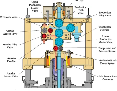
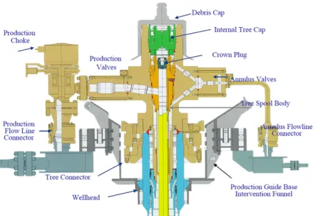
Fig.13:Vertical Xmas tree conceptual layout 42 Fig.14: Horizontal Xmas tree conceptual layout. 43

Fig.15: Jumper conceptual layout. 43

Fig.16: Common jumpers shapes. 44

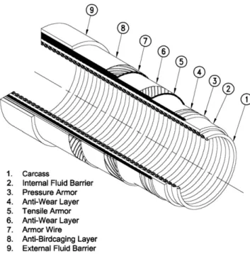
Fig.17: Flexible jumpers layers. 45

Fig.18: Flexible jumper and PLET connection. 45 Fig.19: Vertical tie-in connection end (left) and deployment(right). 46 Fig.20: Horizontal tie-in connection procedure. 47

Fig.21: Horizontal tie-in deployment 47

Fig.22: Subsea GE Manifold. 48

Fig.25: Free hanging riser systems 52 Fig.26: Top tensioned risers deployed in both SPARs and TLPs. 53 Fig.27: Flexible riser connected to a FPSO. 54

Fig.28: Flexible riser layers. 55

Fig.29: Hybrid riser connected to a FPSO. 55

Fig.30: Subsea distribution system. 56

Fig.31: Umbilical, umbilical layers and cables. 57 Fig.32: Asphaltene deposited layer on the internal wall of a pipeline. 58

Fig.33: Deposited Wax layer. 59

Fig.34: Hydrate plug. 61

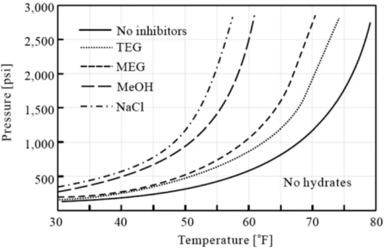
Fig.35: Hydrate crystal structures: type I (left) type II (right). 64 Fig.36: Effect of salt and inhibitors on hydrate forming envelope. 66 Fig.37: Hydrate distribution for each inhibitor type. 67 Fig.38: Flow patterns in horizontal pipes. 70

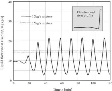
Fig.39: Flow stability at riser base. 71

Fig.40: Slug formation process. 72

Fig.41: Effect of pipeline topography to flow pattern 73

Fig.42: Formation of Riser Slugging 73

Fig.43: Gas lift effect on tubing pressure distribution. 75 Fig.44: Well production against gas injection flow rate and pressure. 76 Fig.45: Worldwide locations for subsea pumping, water injection and separation systems. 78 Fig.46: Conventional separation, pumping and compression conceptual layout. 79 Fig.47: Conventional separation, pumping and compression process layout. 79 Fig.48: Multiphase boosting conceptual layout 80

Fig.50: Effect of pump deployment on system flow matching 80 Fig.51: Pressure profile of natural flow system. 81 Fig.52: Pressure profile of subsea multiphase boosting system. 81 Fig.53: Pressure profile of conventional separation system. 82 Fig.54: Common pump locations and umbilical paths. 84 Fig.55: Volumetric pumps characteristic curves 85 Fig.56: Dynamic pumps characteristic curves 85

Fig.57: Multiphase pumps classification. 86

Fig.58: Phase separation in a rotating channel or an impeller with radial blades. 87 Fig.59: Fluid path in a rotating impeller: black arrow R0 >1; red arrow R0 <1. 88 Fig.60: Accelerations acting on a fluid element in axial flow and secondary flow in an axial

impeller (right). 89

Fig.61: Helico-axial pump. 89

Fig.62: Buffer tank effect on shaft torque. 91

Fig.63: Buffer tank conceptual layout. 91

Fig.64:Rotodynamic pump characteristic at constant GVF and pressure. 93 Fig.65: Rotodynamic pump characteristic at constant GVF and pressure. 93 Fig.66: System characteristic curves for different vapor fractions. 94 Fig.67: Influence of air content on the characteristics of a single-stage pump with inlet

pressure of 2,5 bar. 95

Fig.68: Cross sections of a centrifugal, an hybrid and a helico-axial pump (from right to left). 96 Fig.69: Multiple screw pump (left) and twin-screw pump (right). 97 Fig.70: Twin-screw section. Blue section are the suction channels, whereas the red ones show the outlet flow. Green surfaces are filled with lubricant. 98 Fig.71: Twin screw system section: pump module (left) and electrical motor (right). 98

Fig.73: Ideal volumetric pumping: ideal volumetric pump (top) and ideal pressure profile

(bottom). 100

Fig.74: Real pumping process: actual pump (top) and actual pressure profile. 101

Fig.75: pressure distribution 102

Fig.76: Camera acquired pictures of multiphase multiple-screw pump. 104 Fig.77: High viscosity liquid injection: mixture compression due to liquid compression and

related pressure profile. 106

Fig.78: Effect of injection point location on total flow rate. 107 Fig.79: Sand erosion effect on screw edges (left) and sand velocity map. 107

Fig.80: Progressing cavity pump. 108

Fig.81: OLGA discretization process. 114

Fig.82: Adjust logical solving procedure. 122 Fig.83 :HYSYS Recycle logical operator purpose in solving the HYSYS flowsheet. 122 Fig.84: System hydraulic matching between wells, pump and system characteristic curves.124 Fig.85: Chamber pressure, liquid and gas temperature profiles during the multiphase

compression process in a twin screw pump. N is the rotational speed and 1/N is the fluid

residence time. 125

Fig.86: Slip flow paths in a multiphase twin-screw pump. 127 Fig.87: Frontal conceptual view of a twin-screw chamber and slip flow preferential paths. Thicker green arrows illustrate the preferential paths, while thinner ones illustrate least

preferred ones. 128

Fig.88: Hydraulic irreversibilities (eddies) along the slip flow path. 131 Fig.89: Equivalent flank surface, depth(sf) and width (lf). 132 Fig.90: Experimental multiphase twin-screw pump performance points (Karassik et al., 2001). 133

Fig.91: Chamber volume (green). 134

Fig.94: Other pressure distributions along pump shaft: sensibility to GVF variations

from(Räbiger, Maksoud, Ward, & Hausmann, 2008) and from (Chan, 2009). 139 Fig.95: Simulated system conceptual layout. 141 Fig.96: Pump locations and gas lift injection point in the simulated system. 142 Fig.97: Multiphase pump connection system layout. 146

Fig.98: OLGA simulated system layout. 149

Fig.99: Pump displacement from riser base to manifold and further umbilical length. 185 Fig.100: Energy losses comparison between riser base and manifold located pumps (I

producing year, differential 30 actual bar. 189 Fig.101: Hot diesel circulation path: from production riser to service riser. 194 Fig.102: Preferential gas path: the gas moves towards wells, pushed by buoyancy forces. 198

List of tables

Tab.1: Wells template and wells cluster layouts comparison. 43

Tab.2: Flow assurance study: conceptual procedure. 65

Tab.3: Hydrate host molecules. 70

Tab.4: Subsea multiphase pump requirements. 88

Tab.5: Common material used for surface multiphase pumps 104

Tab.6: Mixture adiabatic temperature against GVF. 109

Tab.7: Main features comparison of TSPs an HAPs for subsea duties. 115

Tab.8: Main features comparison of multiphase boosters for downhole duties. *(elastomer stator). 116

Tab.9: Chisholm’s empirical factor values for Lockhart-Martinelli coefficient prediction. 135

Tab.10: Geometrical dimensions of the simulated pump. 141

Tab.11: Model errors in pump performance prediction. 143

Tab.12: Simulations performed during the first producing year. 148

Tab.13: Simulations performed during the third (first table) and ninth (second table) producing year. 149

Tab.14: Wells properties. 150

Tab.15: Tubing layers properties. 150

Tab.16: Insulated flowline layers properties. 151

Tab.17: Flexible jumper layers properties. 152

Tab.18: Flexible riser layers properties. 153

Tab.19: Natural flow operability map. 156

Tab.20: Gas lift operability map. 156

Tab.21: MPP operability map. 157

Tab.22: MPP+GL operability map. 157

Tab.23: Optimal gas injection rate per scenario. 159

Tab.24: Optimal rated differential pressure per scenario. 160

Tab.28: Standard oil flow rates during pump and gas lift steady state operation. 164

Tab.29: Wells multiphase mass flow rates [kg/s] in MPP strategy. *Grey: slugging operation. 165

Tab.30: Wells multiphase mass flow rates [kg/s] in GL strategy. *Grey: slugging operation. 165

Tab.31: Wells multiphase mass flow rates [kg/s] in MPP+GL strategy. *Grey: slugging operation. 166

Tab.32: Critical times for operators promptness. 168

Tab.33: Riser base cool down times (those obtained considering the 1 bar hydrate formation

temperature are reported in brackets) in the MPP strategy. 174

Tab.34: Jumper base cool down times (those obtained considering the 1 bar hydrate formation

temperature are reported in brackets) in the MPP strategy. 175

Tab.35: Temperature reductions due to cold gas injection at riser base. 176

Tab.36: Riser base available cool down times (those obtained considering the 1 bar hydrate formation

temperature are reported in brackets) in the MPP strategy. 178

Tab.37: Jumper available cool down times (those obtained considering the 1 bar hydrate formation

temperature are reported in brackets) in the MPP strategy. 178

Tab.38: Wellhead and riser base available cool down times. 181

Tab.39: Effective differential pressure for both pump locations. 184

Tab.40: Pump powers for both pump locations.*(bold borders mean that one single pump is operating,

while red cells underline that the pump is operating under slugging conditions). 184

Tab.41: Pump specific powers for both pump locations.*(bold borders mean that one single pump is

operating, while red cells underline that the pump is operating under slugging conditions). 184

Tab.42: Pump location comparison (shaft data) under same actual differential pressure. 185

Tab.43: Pump locations efficiency comparison (bold borders mean that one single pump is operating,

while red cells underline that the pump is operating under slugging conditions). 186

Tab.44: Gas compressors shaft powers in GL strategy. 186

Tab.45: Pump performances for both locations in MPP+GL strategy (I year) 187

Tab.46: Gas compressors shaft power (MPP+GL strategy). 187

Tab.47: Specific powers for each producing strategy.*(bold borders mean that one single pump is

operating, while red cells underline that the pump is operating under slugging conditions). 188

Tab.48: Overall electrical transmission efficiencies for both pump locations and for each transmission

strategy. 192

Tab.49: Power losses during power transmission and pumping process (riser base). 193

Tab.52: Specific electric powers for gas compression 194

Tab.53: Specific electric powers for both pump locations 194

Tab.54: Pump locations overall comparison: electrical powers, overall efficiencies and specific

electric powers. 195

List of graphs

Chart 1: Model predicted pressure profile for a 90 GVF air-water mixture. 131

Chart 2: Model sensibility to GVF variations at 2000 rpm. 138

Chart 3: Experimental and model predicted values matching and comparison. Continuous lines stand

for model predicted trends, while dashed ones for manufacturer provided ones. 142

Chart 4: Model percentage errors in flow prediction. 142

Chart 5: Model pressure distribution along pump shaft: sensibility to GVF variations. 143

Chart 6: Subsea system bathymetry. 154

Chart 7: GVF and pressure profiles for both pump locations. (Rated differential pressure = 60 bar). 161

Chart 8: Steady state maximum standard oil flow rate with pump deployment 162

Chart 9: GVF and pressure profiles for both pump locations (Rated differential pressure = 60 bar) and

gas lift (injected gas flow rate = 15 MMscf/d). 163

Chart 10: GVF and pressure profiles for both pump locations (Rated differential pressure = 60 bar), gas lift (injected gas flow rate = 15 MMscf/d) and pump-gas lift coupling (Rated differential pressure

= 60 bar and injected gas flow rate = 10 MMscf/d). 164

Chart 11: Pressure profile along flowline length during nominal operating conditions (dynamic

pressure profile) and after a shutdown(static pressure profile). 167

Chart 12: Hydrate formation envelopes for different gas compositions (lower flash pressures lead to

heavier components in the vapor phase). 168

Chart 13: Hydrate formation temperature plotted against system geometry. 169

Chart 14: Steady state temperature profiles for both pump locations ( rated differential pressure= 60

bar). 170

Chart 15: Temperature profiles and hydrate formation temperature during a shutdown. (I year, riser

located pump with 60 bar of rated differential pressure). 171

Chart 16: Temperature profiles and hydrate formation temperature during a shutdown. (I year,

manifold located pump with 60 bar of rated differential pressure). 171

Chart 17: Temperature profiles and hydrate formation temperature during a shutdown. (III year, riser

located pump with 60 bar of rated differential pressure). 172

Chart 18: Temperature profiles and hydrate formation temperature during a shutdown. (III year,

manifold located pump with 60 bar of rated differential pressure). 153

Chart 19: Temperature profiles and hydrate formation temperature during a shutdown. (IX year, riser

located pump with 60 bar of rated differential pressure). 173

Chart 21:Temperature profiles during nominal, turndown I and turndown II operational conditions. 176 Chart 22: Temperature profiles and hydrate formation temperature during a shutdown. (I year, gas

flow rate =20MMscf/d ). 177

Chart 23: Temperature profiles during nominal, turndown I, turndown II operations (III year, gas

injection rate: 15 MMscf/d ) 179

Chart 24: Temperature profiles during nominal, turndown I, turndown II operations (III year, gas

injection rate: 15 MMscf/d). 179

Chart 25: Temperature profiles and hydrate formation temperature during a shutdown. (I year, riser located pump with 60 bar of rated differential pressure and gas flow rate =5 MMscf/d).161

Chart 26:Temperature profiles and hydrate formation temperature during a shutdown. (I year,

manifold located pump with 60 bar of rated differential pressure and gas flow rate =5 MMscf/d). 180

Chart 27: Pump power, differential pressure, flow rate for both pump locations. 183

Chart 28: Frictional losses [bar] plotted against pump (riser base located) differential pressure. 189 Chart 29: Frictional losses [bar] plotted against pump (manifold located) differential pressure. 189

Chart 30: Temperature profile after the warm-up procedure. 197

Chart 31: Wellhead jumpers warm-up times in MPP strategy. 198

Chart 32: Wellhead jumpers warm-up times in GL strategy. 199

Chart 33: Wellhead jumpers warm-up times in MPP+GL strategy. 198

1. Introduction

Fig.1: World oil production in MMbbl/d (BP).

World energy demand is keeping growing since 1970 and oil consumption, as main primary energy source, is growing as well. The overall oil production increased consequently and the global oil reserves were expected to decrease at the same rate. However, technological progress and price growth lead to the discovery and the exploitation of new oilfields, which were either unknown or considered too expensive to be exploited.

Fig.2: World oil reserves (left) and reserves/production ratio (right). (BP)

As a result, the ratio between oil production and reserves remained steady during time. Now “easyoil” age is ended and most of new oilfields have been discovered

and maintenance are much more complex and expensive to be performed. Only overcoming these challenges the offshore industry has developed through years. The offshore oil and gas industry started in 1947, when Kerr-McGee completed the first successful offshore well in the Gulf of Mexico (GoM) in 4,6 m of water. The first subsea field was developed in the early 1970 by displacing wellhead and production equipment from topside to seabed, sealing most of the components in a waterproof chamber. Then, produced fluid was conveyed through pipeline to a nearby processing facility, either onshore either offshore located. Subsea systems refer to those systems which have a well and associated equipment below the water surface. System operating up to 200 m (in other words, those reachable by human divers) of water depth are referred as shallow water completions, while those beyond this depth are referred as deepwater ones. If the field is located deeper than 1500 m, it is considered a ultra-deepwater one. Thanks to technology improvements, such as remote control, subsea developments have moved towards deeper waters reaching 3,000 meters in Gulf of Mexico. W ater Depth F eet/ (m) 1940 1950 1960 1970 1980 1990 2000 2010 Year Legend: Platform/Floater Exploration Subsea Denotes Current World Record

0 2,000 1,000 4,000 3,000 6,000 5,000 8,000 7,000 10,000 12,000 11,000 9,000 Present 2011 World Record DP Drilling 10,011' (3,051 m) US GOM, AC 951 Rig: Transocean’s Discoverer Deep Seas

Operator: Chevron

2. Subsea production systems

Subsea oilfields usually are turbidite sandstone formations and show extraction problems because they are characterized by small difference between reservoir and wellhead pressures. Indeed, the reservoir is often close to the seabed, resulting in low reservoir-pressures, while wellhead pressure is usually high due to frictional losses across the pipeline and geodetic pressure difference across the riser.

TYPICAL PRODUCTION AND PUMPING SYSTEMS TOPSIDES SUPPORT EQUIPMENT ON HOST

(REPRESENTATIVE ILLUSTRATION ONLY) Courtesy of INTECSEA Tree Jumpers Subsea Trees Flying Leads Process Jumpers HV Junction Box LV Junction Box Fiber Optic Junction Box

Fiber Optic Junction

Box Subsea Pumping Umbilical

Hydraulic Termination

Assembly LV Junction

Box

Subsea Production Umbilical (Chemicals/Controls for

Trees & Manifolds) Subsea Production

System Power

and Control Equipment Hydraulic

Power Unit

Hydraulic Termination

Assembly Subsea Production Umbilical

Chemical Injection Unit Subsea Pump Barrier Fluid Hydraulic Power Unit Subsea Pump Power and Control

Equipment MV to HV Step-Up Transformer Subsea Pumping Umbilical Semi Floating Production Facility SUTA

Subsea boosting station on a suction pile. Pump & stepdown transformer

are retrievable components.

HV flying leads (x3) terminated in subsea step-down transformer (Primary is HV/ Secondary is MV), EFL (x1), and HFL (x1);

single line shown for clarity Production Flowline PLET Subsea Pump Manifold Subsea Production Manifold

SUTA Integrating HV Wet Mate Power Connector and MQC Stab Plates for Booster Utilities

ILLUSTRATION ACRONYMS:

EFL Electrical Flying Lead

HFL Hydraulic Flying Lead

HV High Voltage

LV Low Voltage

MQC Multi-Quick Connect

MV Medium Voltage

PLET Pipeline End Termination

SUTA Subsea Umbilical Termination Assembly

GENERIC SUBSEA BOOSTING SYSTEM

Background Illustration Courtesy of Chevron Energy Technology Corporation

Fig.4: Subsea tieback system development.

A subsea production system can be made of a single satellite well or several wells linked to a manifold with a flowline conveying the fluid to a fixed platform, FPSO (Floating Production, Storage and Offloading), or onshore facility. When some reservoirs cannot be reached due to geometry and water depth, subsea production systems are used to extend existing platforms. Subsea production systems can be divided depending on whether the Xmas tree arrangement has been located:

• Dry tree systems, when the Xmas tree is topside located; • Wet tree systems, when the Xmas tree is subsea located.

The main parts of a subsea production system usually are: • Subsea completed wells;

• Seabed wellheads and Xmas trees; • Subsea tie-in to flowline systems; • Umbilicals;

• Riser;

• Subsea manifolds and jumpers;

• Subsea equipment and control facilities.

In the following chapters, each system component will be briefly described.

2.1. Subsea developments

Fig.5: Dry tree and wet tree systems layout.

Subsea systems developments can be divided on whether the Xmas tree is located:

• Dry tree development, when the Xmas tree is located on a surface structure. They are preferred when a fixed platform, a tension leg platform (TLP) or SPAR is available, due to their reduced sensibility to the wave movement. Thanks to their accessibility, they reduce the maintenance costs and simplify

are starting to establish as alternative solution to wet tree wells clusters development. This combination can eventually become an interesting technology in the Gulf of Mexico as the FPSO philosophy becomes progressively widespread. To date, existing (or actually planned) WHP systems are based on TLP concept.

• Wet tree development, when the Xmas tree is located on the seafloor. Its does not require a fixed host facility and is particularly appreciated for long subsea tieback applications. For its nature, it has lower CAPEX and higher OPEX than dry tree development. Two main layouts of wet tree development can be identified: subsea wells clusters and direct access wells. Wet tree development can be accomplished with three different types of riser, steel catenary, top tensioned and flexible risers.

To date, most of operators has felt more comfortable in dealing with wet tree developments for deepwater systems and considers dry tree ones more suitable for shallow water fields.

2.1.1.1. Wet tree developments: direct access wells

This development allows to directly perform workover and drilling activities from the production support, which is very useful in marginal field development.

2.1.1.2. Wet tree developments: wells clusters

This production solution is the most efficient and cost-effective one, either suitable for close located wells, either for remote ones, linked to an already existing infrastructure through a long distance subsea tie-back. The infrastructure is, in most of the cases, a FPSO unit.

2.1.2. Stand alone development

This solution is viable when reservoir size justifies the economic development of topside processing facilities, which is further verified for gas fields. Thus, the choice of whether developing a stand-alone or tie-back system is dictated by economic parameters (as discussed in paragraph 2.1.3). Stand alone developments are generally divided accordingly to the type of facility connected to the field.

2.1.2.1. Fixed platforms

These platforms best suite big reservoir and shallow (up to 520m) developments. Indeed, these platforms are built on steel legs anchored directly onto the seabed (thus shallow water applications), supporting a deck with space for drilling rigs,

Various types of structure are used: steel jacket, concrete caisson, floating steel, and even floating concrete.

2.1.2.2. Compliant towers

The main component of these platforms is a narrow tower, supported by a foundation on the seafloor. This tower is more flexible than the fixed platform one. This flexibility allows to operate in much deeper waters, as they can sustain lateral deflections due to forces exerted by wind and sea. Petronius is actually the deepest compliant tower in world and is located in 531 m of water depth.

Fig.6: Deepest semi-submersible platforms in the world. 2.1.2.3. Semi-submersible platforms

Semi-submersible platforms are not supported by a foundation linked to seabed, whereas they are equipped with large hulls (column and pontoons), which allow the structure to float. Semi-submersibles were used in water depths up to 2500 m. They differ from tensioned-legs platforms in the mooring mechanism: they are generally anchored by combinations of chain, wire rope or polyester rope. Actually, the deepest platform is Independence Hub, which is located in 2415m of water depth.

2.1.2.4. Jack-up platforms

These platforms are suitable for small reservoirs in shallow waters. Indeed, thanks to their unique feature, they can be jacked up above the sea level by

1,933 m 6,340 ft US GOM 1,849 m 6,065 ft US GOM Thunder Horse 2008 1,707 m 5,599 ft Brazil P-55 2009

Semi-FPS/FPUs – 15 Deepest Facilities Sanctioned, Installed or Operating

Na Kika 2003 1,980 m 6,494 ft US GOM 2,134 m 7,000 ft US GOM Blind Faith 2008 Jack/St. Malo 2014 1,845 m 6,050 ft US GOM Thunder Hawk 2009 1,795 m 5,888 ft Brazil P-52 2012 1,700 m 5,576 ft Brazil P-56 2010 1,189 m 3,900 ft Malaysia Gumusut Kakap 2012

2.1.2.5. Floating production systems (FPS)

FPSs are large monohull structures, which are often derived from ship ones, equipped with processing facilities. There are different technical solutions such as FSOs, FSUs, and FPSOs. They often offer nice economic advantages, thanks to their similarities to ships in the building process.

Fig.7: Deepest TLPs in the world. 2.1.2.6. Tension leg platforms (TLPs)

TLPs are floating structures, similar to semi-submersible platforms, tethered to the seabed in order to avoid vertical movements of the structure. The structure is tethered to seabed throughout four tension legs, each one corner located. The tension leg is made of tubular steel members, called tendons. The tendon system is highly tensioned due to excess of the platform hull buoyancy. TLPs are best suited for applications between 100m and 1500m of water depths.

1,178 m 3,863 ft Angola Kizomba B 2005 1,178 m 3,863 ft Angola Kizomba A 2004 1,581 m 5,187 ft US GOM Big Foot 2014 1,425 m 4,674 ft US GOM Magnolia 2005 1,280 m 4,200 ft US GOM Neptune 2007 1,311 m 4,300 ft US GOM Marco Polo 2004 1,333 m 4,373 ft US GOM Shenzi 2009 1,200 m 3,937 ft Brazil Papa Terra P-61

Fig.8: Deepest SPARs in the world. 2.1.2.7. Spar platforms

There are different types of spar used, classified by the platform hull: • Cylindrical hull: This is the very first version of these floating platforms;

• Truss spar: in these platforms, the upper buoyant hull is connected to bottom stabilizer ballast through a midsection, composed of truss elements. This is, actually, the most widespread spar platform;

• Cell spar: cell spars, for example the Red Hawk, are built from multiple vertical cylinders.

Spars are similarly moored to the seabed as TLPs, but they do not have either tension legs either a tendon system. Spars are tethered to seabed through a conventional catenary mooring line. Shell Perdido is actually the deepest spar in the world and is located in Gulf of Mexico in 2383 m of water depth.

1,616 m 5,300 ft US GOM 1,515 m 4,970 ft US GOM 1,348 m 4,420 ft US GOM Mad Dog 2005 1,710m 5,610 ft US GOM Devils Tower 2004 1,463 m 4,800 ft US GOM Hoover/Diana 2000 1,653 m 5,423 ft US GOM Horn Mountain 2002 Constitution 2006 Red Hawk 2004 2,383 m 7,817 ft US GOM Perdido 2010

2.1.3. Subsea tieback development

Fig.9: Subsea tie back to FPSO.

The exploitation of deepwater reservoirs has been feasible only when huge amount of hydrocarbons could be recovered, otherwise the capital cost investment for the establishment of these subsea systems could not be justified. As consequence of that, marginal oilfields have been often ignored. Recently, operators have found in tie-back developments the key solution to economically exploit these fields, by connecting them to an existing processing facility and saturating the spare processing capacity.

Subsea tiebacks are denoted by lower capital cost investments and by high technical complexity. This emerging solution is continuously spreading out and establishing all over oil&gas industry, reaching deeper and farther fields. Indeed, tieback economics is mainly governed by the following parameters:

• Distance from existing installation; • Water depth;

• Recoverable volumes, reservoir size, and complexity;

• Potentially lower recovery rates from subsea tie-backs versus standalone development, due to limitations in the receiving facility’s processing systems and to higher back pressure on wells (longer distance to be covered).

Shallow Deepwater Ultra Deepwater US MMS Definitions: 0' 1,000' 2,000' 3,000' 4,000' 5,000' 6,000' 7,000' 8,000' 9,000' 10,000' 0 Miles 5.0 10.0 15.0 20.0 25.0 30.0 35.0 40.0 45.0 50.0 55.0 60.0 65.0 70.0 75.0 80.0 85.0 90.0 95.0 100.0 (0 km) (8.05 km) (16.1 km) (24.1 km) (32.2 km) (40.2 km) (48.3 km) (56.3 km)

Tieback Distance Miles (km)

(64.4 km) (72.4 km) (80.5 km) (88.5 km) (96.6 km) (104.6 km) (104.6 km) (112.7 km) (120.7 km) (128.7 km) (136.8 km) (144.8 km) (152.9 km) (160.9 km) World Record Subsea Tiebacks s Sanctioned, Installed, Operating or Future Tiebacks (Water Depth vs. Tieback Distance) s As of March 2011

Short Short Oil Subsea Tiebacks: Gas Subsea Tiebacks:

Conventional

Conventional

Long Distance Tieback (LDT)

Long Distance Tieback (LDT)

Future Oil Subsea Tiebacks Gas Subsea Tiebacks Future Gas Subsea Tiebacks

Legend: Oil Subsea Tiebacks

Oil Subsea Tieback Experience Limit Gas Subsea Tieback Experience Limit Denotes Current World Record for Installed Tiebacks

Mariner’s Bass Lite

56.0 (90.1 km) 6,750' (2,057 m) Shell’s Oregano 8.0 (12.9 km) 3,400' (1,036 m) Shell’s Habanero 11.5 (18.5 km) 2,015' (614 m) Anadarko’s Merganser 14.7 (23.7 km) 7,934' (2,418 m) Anadarko’s Mondo 12.0 (19.3 Km) 8,340' (2,542 m) Anadarko’s Spiderman 24.0 (38.6 km) 8,113' (2,473 m) Anadarko’s Jubilee 20.6 (33.1 km) 7,868' (2,675 m) Anadarko’s Atlas NW 22.0 (35.4 km) 8,856' (2,700 m) Anadarko’s Atlas 24.9 (40.1 km) 9,005' (2,745 m) Anadarko’s Vortex 24.5 (39.4 km) 8,381' (2,555 m) Anadarko’s Cheyenne 44.7 (72.0 km) 9,014' (2,748 m)

Dominion Expl.’s San Jacinto

34.0 (54.7 km) 7,868' (2,399 m) BP’s King 17.0 (27.4 km) 5,334' (1,626 m) Shell’s Manatee 17.0 (27.4 km) 1,940' (591 m) BP’s Aspen 16.0 (25.8 km) 3,150' (960 m) Shell’s Macaroni 11.8 (19.0 km) 3,685' (1,123 m) Shell’s Crosby 10.0 (16.1 km) 4,393' (1,339 m)

Record Water Depth for Oil SS Tieback

Record Distance for Oil SS Tieback Shell’s Europa 20.0 (32.2 km) 3,900' (1,189 m) ATP’s Ladybug 18.0 (29.0 km) 1,355' (413 m) 69.8 km ExxonMobil’s Mica 29.0 (46.67 km) 4,350' (1,326 m) Pioneer’s Falcon 30.0 (48.3 km) 3,400' (1,036 m) BP’s Machar 22.0 (35.3 km) 738.1' (225 m) Statoil’s Mikkel 24.3 (39.2 km) 738' (225 m)

Noble’s Lost Ark

27.0 (43.5 km) 2,700' (823 m) Mariner’s Pluto 28.6 (46.0 km) 2,900' (884 m) Pioneer’s Tomahawk 35.0 (53.1 km) 3,500' (1,067 m) Chevron’s Gemini 28.0 (45.1 km) 3,488' (1,063 m) Shell’s Mensa 68.0 (109.4 km) 5,300' (1,615 m)

Record Distance for Gas SS Tieback

Total’s Canyon Express

57.0 (91.7 km) 7,210' (2,198 m) Record Water Depth for Gas SS Tieback Shell’s Coulomb 27.0 (43.5 km) 7,570' (2,307 m) BG International’s Simian/Sienna 68.4 (110.0 km) 3,445' (1,050 m) BG International’s Scarab/Saffron 55.9 (90.0 km) 2,040' (622 m) Pioneer’s Raptor 40.0 (64.4 km) 3,500' (1,067 m) Pioneer’s Harrier 47.0 (75.6 km) 4,200' (1,280 m) 143 km 89.0 9,356' 43.4 2,118.2 m 2,748 m ExxonMobil’s Madison 7.0 (11.26 km) 4,851' (1,479 m) ExxonMobil’s Marshall 7.0 (11.26 km) 4,356' (1,328 m) 9,014'

Norsk Hydro’s Ormen Lange

74.6 (120.0 km) 3,609' (1,100 m)

Statoil’s Snøhvit 89.0 (143 Km) 1,131.9' (345 m) Shell’s Penguin A-E

43.4 (69.8 km) 574' (175 m) Shell’s Keppler 11.8 (18.96 km) 5,759' (1,755 m) Shell’s Silvertip (2) 9.0 (14.4 km) 9,356' (2,852 m) Shell’s Tobago 6.0 (9.6 km) 9,627' (2,934 m) Shell’s Ariel 4.74 (7.628 km) 6,240' (1,902 m)

Shell’s East Anstey

11.0 (17.77 km) 6,590' (2,009 m) Shell’s Herschel 12.8 (20.7 km) 6,739' (2,054 m) Shell’s Fourier 16.8 (27.1 km) 6,950' (2,118.2m) Statoil’s Q 11.2 (18 Km) 7,960' (2,427 m)

Notes: 1. Assistance from Infield Systems Ltd. (www.infield.com)

Fig.10: World record subsea Tiebacks

The former graph shows how tie-back length and water depth have increased during time, thank to strong improvement in the subsea technology and economics, making feasible the exploitation of marginal fields.

The marginal field can either be linked to a FPSO (Fig. 9), a fixed platform or to an onshore facility, generally throughout a dual flowline with an end-to-end loop, which are customarily built for subsea tie-backs and provide a full circuit for the pig, which can travel from the processing facility to the manifold then turn and come back to the facility.

The tieback development should deliver the conveyed fluid at temperatures above the solid formation ones (such as hydrate formation, cloud point and wax appearance temperatures). Concerning this issue, pipe insulation and heat retention strategies represent a key design feature. Indeed, solid formation (and consequent solid structures building up) can lead to pipe occlusion and catastrophic failures.

During the project development, it is essential to assess whether the reservoir energy can overwhelm the backpressure and lead the hydrocarbon to the processing facility with acceptable flow rates. To this purpose, multiphase subsea boosting offers many advantages (better discussed in the following chapters). Riser-base gas injection is another interesting solution to reduce back pressure by lightening the fluid column in the riser. A further advantage is to reduce slugging and to provide the possibility of depressurizing the line during a shutdown.

2.2. Subsea layouts

Depending on the field characteristics and specifications, different common layouts can be used to develop the subsea system. The well location layout is generally a trade-off between the need of space, for oil recovery maximization, against cost saving benefits due to well grouping in clusters. In the following paragraphs, four main subsea layouts are briefly exposed in following paragraphs and illustrated in the picture below.

Fig.11: Subsea conceptual layouts. 2.2.1. Satellite well layout

A satellite well is a single subsea well. A satellite well layout means that each well is independently connected to the process facility. This solution is preferred when the distance between wells is high.

2.2.2. Clustered Satellite Wells

When distance between wells is small, it is convenient to collect all the reservoir produced fluid in a single flowline. Wells are connected by means of a manifold. This arrangement allows cost saving both for the flowlines and for the umbilicals.

2.2.3. Production Well Templates

While well clusters layout aims to connect many close wells, a well template is designed to closely locate a group of wells. Well templates are prefabricated steel structures which accommodate both well heads and manifold. They can support from two to twelve wells. The number of wells, a template could host, is simply limited by reservoir considerations and by template weight, which can be handled by the installation vessel. The choice of whether applying a cluster o

Processing* facility* Well* Tie2back* Manifold* Template* Satellite*well* Wells* Template** Clustered* Wells* Daisy* Chain*

Well  template  layout  advantages  and  disadvantages  compared  to  cluster  layout Well  template  layout  advantages  and  disadvantages  compared  to  cluster  layout

Advantages Disadvantages

• Wells  are  precisely  spaced.   • Design  and  fabrica4on  4me  may  be  _{longer  due  to  greater  complexity.}   • Manifold  piping  and  valves  can  be  

incorporated.   • There  may  be  safety  concerns  related  to  simultaneous  drilling  and   • Piping  and  umbilical  jumpers  between  the  

trees  and  manifolds    prefabricated  and   tested  prior  to  deployment  offshore.   • Piping  and  umbilical  interfaces  are  less  

expensive  than  for  clustered  wells.   • Installa4on  4me  is  reduced  by  

modularizing  much  of  the  equipment.   • Short  flowline  piping  distances  (compared  

to  a  cluster)  reduce  the  problems  

associated  with  flow  assurance  (e.g.,  wax   and  hydrate  forma4on).

Tab.1: Wells template and wells cluster layouts comparison. 2.2.4. Daisy Chain

When there are one or more wells, which are far located by another group of wells, it is possible to connect both groups of wells through a single subsea flowline. This layout, which connects two or more well hubs with a single flowline, is called Daisy Chain. When this layout is used, it is possible to create a continuos loop, so that the flow line is piggable, leading to the following advantages:

• Round trip pigging;

• Possibility to redirect both production flows into a single flowline if the second is damaged;

Most of Daisy Chain configuration advantages can be summed up as follows: • Similar to a single satellite well, cost is upfront: only when the installation is

performed the cost is faced by the operator; • Flowlines sharing may be possible;

• Potential damage from dropped objects is limited; • Simultaneous production and drilling.

Disadvantages of Daisy Chain wells include: • Subsea chokes possibly required on each well;

• Relocation of the drilling rig vessel in order to reach another well.

2.3. Subsea Processing

Subsea processing refers to those physical or chemical treatments subsea performed to improve the system flow assurance and performance. Subsea processes include: • Subsea boosting; • Subsea separation; • Solids management; • Heat exchange; • Gas treatment; • Chemical injection.

Most of the times, subsea processing is required in order to exploit the field (chemical injection to avoid hydrate formation or gas injection to mitigate severe slugging), but often it simply provides some advantages. For instance, the deployment of a subsea multiphase pump allows to increase the oil production or to extend the field life.

3. Subsea Components

Hereafter, a brief description of main subsea components will be carried out. The description includes the following subsea equipment:

• Wellhead;

• Subsea Xmas tree; • Jumper;

• Manifold; • Subsea valve;

• Pipeline end termination (PLET); • Subsea pipeline;

• Riser;

• Distribution system; • Umbilical.

3.1. Wellhead

Wellhead is the pressure-containing component at the surface of an oil well. It supports casing strings and the subsea tree after completion; its function is mainly to operate as pressure-containing anchoring point on the seabed for the drilling and completion operations. It can be located on the offshore platform or onshore (surface wellhead); if it is located on the seabed, it is called subsea wellhead.

3.1.1. Subsea wellhead

A subsea wellhead is made of the following components:

• Wellhead housing: it is the main pressure-containing component of the subsea well head. It supports and seals the casing hangers and shifts external loads to the conductor housing;

• Conductor housing: it accommodates most of the wellhead equipment (mainly pipes);

• Annulus seals: they simply seal one environment from another, especially for isolating the geological formation;

• Guide base: it is a structure for guiding equipment into the wellhead. There are different kinds of subsea wellhead guide bases, depending on the subsea system conceptual layout. For instance, a Template-Mounted Guide Base (TMGB) is required if production well template layout is used. Single-Well or Cluster Production Guide Base (SWPGB) is suitable for both cluster and single-well configurations.

Fig.12:Wellhead cross section.

3.2. Subsea Tree

A subsea Xmas tree is an assembly of valves and spools (whose geometry resembles a Christmas tree and for such reason is called Christmas tree, Cross tree, X-tree, or just tree), used to control the flow rate of the well. They are also used for other auxiliary functions, such as:

• Chemical injection; • Water/gas injection; • Well intervention;

Wellhead to casing hanger Metal Seal assembly

Wellhead to casing hanger Metal Seal assembly Wellhead to casing hanger

Metal Seal assembly

High strength load shoulder Bypass Area

Passive Pre-loaded

lockdown system 13 3/8” casing hanger 10 3/4” casing hanger

7” casing hanger – For Glenelg the tubing hanger is at this elevation and replaces the 7” casing hanger

18 ¾” HP wellhead housing 30” conductor 20” casing 13 3/8” casing 10 3/4” casing C Annulus B Annulus A Annulus

Subsea Xmas trees are classified on their orientation layout: they can be either vertical either horizontal trees.

3.2.1. Vertical Xmas tree

Vertical Xmas trees (VXTs) have vertical aligned master valves located above the tubing hanger. VXTs are definitely widespread thank to their lower cost (five to seven times lower than horizontal ones) and to their versatility. Indeed, they can be also deployed after well completion.

Fig.13:Vertical Xmas tree conceptual layout

The former picture illustrates the essential components of a VXT. As can be noticed, master valves are vertically aligned, as the production swab valve is. Another advantage of the vertical Xmas tree is that it can be retrieved without having to recover the downhole completion.

3.2.2. Horizontal Xmas Tree

Horizontal Xmas trees (HXTs) have found many applications in subsea fields, undermining VXTs supremacy. Indeed, they are lighter and more suitable for wells requiring frequent work-over. They allow simple well intervention thank to their valves disposal and electrical submersible pumps downhole deployment, thanks to the absence of the swab valves.

• Lower production master valve (LPMV);

• Production wing valve (PWV);

• Production swab valve (PSV)

• Crossover valve (XOV);

• Annulus master valve (AMV);

Material Class

Minimum Material Requirements Body, Onnet, End, and

Outlet Connections

Pressure-Controlling Parts, Stems, and Mandrel Hangers

AA e General service Carbon or low-alloy steel Carbon or low-alloy steel BB e General service Carbon or low-alloy steel Stainless steel

CC e General service Stainless steel Stainless steel

DD e Sour servicea Carbon or low-alloy steela Carbon or low-alloy steelb EE e Sour servicea Carbon or low-alloy steela Stainless steelb

FF e Sour servicea Stainless steela Stainless steelb

HH e Sour servicea CRAsb CRAsb

a_{As defined by NACE MR 0175[7].} b

In compliance with NACE MR 0175[7].

Fig.14: Horizontal Xmas tree conceptual layout.

Another difference between VXTs and HXTs is the tubing hanger location. While in VXTs the tubing hanger is located on the wellhead, in HVTs it is installed on the tree itself. Thus, it is absolutely necessary HXTs to be installed before the well completion, otherwise VXTs should be deployed.

3.3. Jumpers

Subsea jumpers are used to link two different subsea components, such as a manifold or a PLET, and allow the transported fluid to flow from one to another component. Their shape is aimed to accommodate thermal expansion during transient conditions.

Fig.15: Jumper conceptual layout.

There are two different kinds of subsea jumpers: • Rigid jumpers;

• Flexible jumpers;

• Annulus access valve (AAV) or annulus swab valve (ASV); • Annulus wing valve (AWV);

• Pressure and temperature sensors (PT, TT, PTT, etc.); • Tree connector;

• Conventional tubing hanger system.

Typical components of a horizontal Xmas tree, as illustrated in

Figure 22-22, are as follows: • Tree debris cap;

• Tree body;

• Internal tree cap (or upper crown plug); • Crown plug (or lower crown plug); • Production master valve (PMV); • Production wing valve (PWV); • Annulus access valve (AAV); • Annulus master valve (AMV); • Annulus wing valve (AWV); • Crossover valve (XOV); • Sensors (PT, TT, PTT, etc.); • Tree connector;

• Tubing hanger system.

Figure 22-22 Typical Components of an HXT

3.3.1. Rigid Jumpers

A rigid jumper is mainly made of a steel pipe and mechanical connections at each end for components linkage. The jumper is required to resist to the combined effect of internal pressure, external bending, torsion, tensile, thermal, and installation loads.

Rigid jumpers may have different configurations, such as “M” shaped or “U” shaped. The “M” shape also can be divided in categories depending on the connection configurations; indeed, it can be linked through bends or through elbow (see paragraph 3.3.3).

Fig.16: Common jumpers shapes.

The main concern on rigid jumpers is the installation procedure. Once the components to be connected are permanently deployed, their distance is measured or calculated. Then the connecting jumper is tailored on the measured length and equipped with coupling hubs on the ends. Once the jumper has been manufactured, it is delivered to the required location. Afterwards, the jumper is lowered and linked with the other two components and tested.

Measurements are absolutely critical for jumpers deployment, indeed if they are not precisely performed or if the components location changed from the previous one, new jumpers may need to be fabricated. Jumper design should take into account the changes in dimensions occurring when the component is lowered below the sea level. Indeed, thermal expansion and shape deformation, due to a load reduction induced buoyancy forces, definitely affect the jumper geometry.

3.3.2. Flexible Jumpers

Flexible jumpers are made of two connectors and a flexible pipe. The flexible connector is a layered set of concentric pipes which provide the physical properties required to face the flexible jumper requirements:

• High-temperature resistance;

• Suitability for dynamic service and strong thermal dilatations; • Fatigue resistance;

• High resistance to collapse; • Low U-value.

The flexible pipe is generally composed of many layers which can move when the pipe is flexed, in order to improve the fatigue resistance. Layers have three main goals:

• Mechanical resistance; • Thermal insulation; • Corrosion resistance.

Fig.17: Flexible jumpers layers.

The main advantage of flexible jumpers is their simplified procedure during the length specification and installation. Indeed, length specification is not required to be so accurate as in the rigid jumper case. As long as the flexible jumper is longer than the distance between the two components to be connected, the installation can be successfully completed.

Fig.18: Flexible jumper and PLET connection.

shown in Figure 21-7. The FSHR consists of a vertical steel pipe (riser) tensioned by a near-surface buoyancy can with a flexible jumper con-necting the top of the riser and the FPSO. An M-shaped rigid jumper is used to connect the vertical riser and a PLEM.

Figure 21-6 Flexible Jumper Configuration

Figure 21-7 Rigid and Flexible Jumpers Used in FSHR System[4]

Subsea Connections and Jumpers 671

3.3.3. Tie-in systems

A tie-in system allows to connect the jumper to a manifold or to a PLET. Tie-in systems used to be mainly horizontal, since subsea development were carried out in shallow waters with the auxiliary help of divers. Since subsea engineering has moved towards deeper waters, the development of vertical tie-in systems guided by control remote units has occurred. Actual horizontal tie-in systems need ROVs (Remote Operator Vehicles) auxiliary help to be installed in deep water oilfields.

3.3.3.1. Vertical tie-in systems

Vertical jumpers are often rigid “U-inverted” shaped jumpers. At both ends of the jumper a downward oriented connector is equipped, which is thought to fit the other components vertical hubs. Vertical connections are installed directly onto the receiving hub during tie-in, as shown in the following picture.

Fig.19: Vertical tie-in connection end (left) and deployment(right). 3.3.3.2. Horizontal tie-in systems

Most of the horizontal connection systems are based on mechanically fastened flange joints. Horizontal tie-in systems offer some interesting advantages against the vertical ones:

• Low possibility of being hooked by anchors or fisheries thanks to the lower geometrical profile;

• Longer tie-in life;

• Simple seal substitution;

Vertical Tie-in assisted by V-CAT

Subsea Tie-in Systems

Subsea flowlines are used for the transportation of crude oil and gas from subsea wells, manifolds, off-­shore process facilities, loading buoys, S2B (subsea to beach), as well as re-­injection of water and gas into the reservoir. Achieving successful tie-­in and connection of subsea flowlines is a vital part of a subsea field development.

Subsea fields are developed using a variety of tie-in solutions. Over the past decade, FMC Technologies has developed a complete range of horizontal and vertical tie-in systems and associated connection tools used for the tie-in of flowlines, umbilicals and jumper spools sizes 2” - 36” and for single and multi-bore application. FMC’s horizontal and vertical tie-in systems have been extensively installed in many of the deepest, highest pressure and largest diameter subsea applications around the world.

Vertical Tie-­in Systems

Vertical connections are installed directly onto the receiving hub in one operation during tie-in. Since the Vertical Connection System does not require a pull-in capability, it simplifies the tool functions, provides a time efficient tie-in operation and reduce the length of Rigid Spools.

Stroking and connection is carried out by the the Connector itself, or by the ROV operated Connector Actuation Tool (CAT) System.

Vertical Tie-in Systems