Politecnico di Milano
SCHOOL OF INDUSTRIAL AND INFORMATION ENGINEERING Master of Science in Computer Science and Engineering
MASTER THESIS
A General Approach to Value Identification of
Large Scale Geospatial Data
Supervisor
Prof. Marco Brambilla Co-Supervisor
Prof. Ernestina Menasalvas Ruiz Prof. Alessandro Bogliolo
Candidate Gioele Bigini Matr.898741
Virtutibus Itur Ad Astra 9th book of the Aeneid
Contents
1 Introduction 1
1.1 Context . . . 1
1.2 Problem Statement . . . 1
1.3 Proposed Solution . . . 2
1.4 Structure of the Thesis . . . 3
2 Background 5 2.1 Internet of Things . . . 5
2.1.1 A Bit of History . . . 5
2.1.2 Challenges . . . 6
2.2 Big Data . . . 7
2.2.1 Data Sets Growth . . . 7
2.2.2 Challenges . . . 8
2.3 Mobile Crowdsensing . . . 8
2.3.1 Data Collection . . . 9
2.3.2 Challenges . . . 9
2.3.3 Architecture . . . 10
2.4 Libraries and Tools . . . 10
2.4.1 Jupyter and Python . . . 10
2.4.2 Apache Spark . . . 11
2.4.3 Google Cloud Platform . . . 12
2.4.4 QGIS . . . 13
3 Related Works 15 3.1 Mobile Crowdsensing Applications . . . 15
3.1.1 Data Collection and Processing Workflow . . . 15
3.1.2 Real-World Applications . . . 18
3.1.2.1 Crowdsensing for the common interest . . . 19
3.1.2.2 SmartRoadSense . . . 19
4 The General Approach for Value Identification 23 4.1 The Concept of Value . . . 23
4.2 The Proposed Approach . . . 24
4.3 Exploratory Analysis . . . 25
4.3.1 Data set . . . 25
4.3.2 Insights . . . 25
4.4 Outcome Definition . . . 26
4.5 Pre Processing . . . 27 4.6 Processing . . . 28 4.7 Visualisation . . . 29 5 Implementation Experience 31 5.1 Exploratory Analysis . . . 31 5.1.1 Data set . . . 31 5.1.2 Row Attributes . . . 32 5.1.3 Retrieving Informations . . . 33 5.1.4 Insights . . . 34 5.2 Outcome Definition . . . 35 5.3 Pre Processing . . . 35 5.3.1 Spatial Query . . . 36 5.4 Processing . . . 39 5.4.1 Anomalies Detection . . . 39
5.4.2 Usage Trend Metric . . . 43
5.4.3 Data Recency Metric . . . 45
5.4.4 Data Quantity Metric . . . 47
5.5 Visualisation . . . 48
5.5.1 Crossed Visualisation . . . 49
6 Experiments And Discussion 51 6.1 Local vs Cluster Solution . . . 51
6.1.1 Local Optimisation . . . 52
6.1.2 Cluster Implementation . . . 54
6.2 Metrics . . . 57
7 Conclusions 63 A Appendix 65 A.1 Jupyter Notebook on Google DataProc . . . 65
A.2 Anomalies Detection . . . 69
A.3 Data Quantity . . . 70
A.4 Data Recency . . . 70
A.5 Usage Trends . . . 70
Acronyms 73 Bibliography 75 References cited in the text . . . 75
Publications and Manuals . . . 75
List of Figures
2.1 General Mobile Crowd Sensing Architecture . . . 10
2.2 Spark Job Flow . . . 11
3.1 MCS Application Workflow . . . 15
3.2 SmartRoadSense Process Flow . . . 20
4.1 Example of bad data collection . . . 26
4.2 Municipalities Selected through Spatial Query in QGIS . . . 28
4.3 Example of Anomalies in a Time Series . . . 29
4.4 Example of Visualisation with Plotly . . . 29
5.1 Measurements distribution for road 97464677 . . . 34
5.2 JSON format after Pre Processing phase . . . 39
5.3 Sample Time Series . . . 40
5.4 Forward Fill on Sample Series . . . 40
5.5 Backward Fill on Sample Series . . . 41
5.6 Corrected Sample Series . . . 41
5.7 New time series originated by the corrected one . . . 42
5.8 Removing anomalies through Forward Filled Series . . . 42
5.9 New time series filled with Linear Interpolation . . . 42
5.10 Removing anomalies through Linear Filled Series . . . 42
5.11 Time series cleaned of the anomalies . . . 43
5.12 Examples of different trend cases . . . 43
5.13 All the municipalities of Marche Region in Italy . . . 44
5.14 Trend of Acqualagna Municipality . . . 45
5.15 Recency Decaying Window . . . 46
5.16 Usage Trends Metric . . . 48
5.17 Data Recency Metric . . . 48
5.18 Data Quantity Metric . . . 49
5.19 Crossed Metrics Result . . . 49
6.1 Pre Processing Algorithm Core . . . 53
6.2 Optimised Pre Processing Algorithm Core . . . 53
6.3 Ancona and Osimo Municipalities Study Case . . . 57
6.4 Ancona (on top) and Osimo (bottom) Municipalities Trends . . . . 58
6.5 Fano/Macerata municipalities with their recency and quantity . . . 59
6.6 Fano (on top) and Macerata (bottom) Municipalities Recency and Quantity . . . 59
6.7 The municipalities of Urbino, Ancona and Ascoli Piceno . . . 60
List of Tables
3.1 SmartRoadSense Open Data Schema . . . 21
5.1 Metrics Explained . . . 48
6.1 Local Execution Results . . . 52
6.2 Optimised Local Execution Results . . . 54
6.3 DataProc Cluster Configuration . . . 54
6.4 Cluster Execution Results and Costs . . . 57
Listings
5.1 Evaluating RAM Occupation . . . 33
5.2 Plotting exploration’s results . . . 33
5.3 Polygon and Point Objects . . . 36
5.4 Transformed and Cached Dataset . . . 37
5.5 Date convertion function . . . 37
5.6 From Hex to Lat/Long . . . 37
5.7 Processing function . . . 38
5.8 Spatial Query . . . 38
5.9 Trend Value Function . . . 45
5.10 Date interval for Recency . . . 46
5.11 Data Recency Value Function . . . 47
5.12 Data Quantity Function . . . 47
6.1 Read GeoJSON From Bucket . . . 55
6.2 Start Processing . . . 55
6.3 Upload Results to Google Cloud Storage . . . 56
A.1 Import Libraries . . . 65
A.2 View SparkContext . . . 65
A.3 Read GeoJSON From Bucket . . . 65
A.4 Load Data . . . 66
A.5 Define functions for Processing . . . 66
A.6 Take Regions Borders . . . 66
A.7 Start Processing . . . 67
A.8 Upload Results to Google Cloud Storage . . . 68
A.9 Function Definitions for Anomalies Detection . . . 69
A.10 Defining Quantities . . . 70
A.11 Defining Recency . . . 70
A.12 Defining Trend . . . 70
Sommario
Oggi la maggior parte dei dispositivi mobili registra continuamente informazioni come dati geo-spaziali. Grazie all’avvento dell’Internet delle Cose, essi stanno gradualmente dominando il settore dei big data. Un’applicazione che si occupa di collezionare questo genere di dati è SmartRoadSense, un app mobile che è stata sviluppata con lo scopo di collezionare dati geo-spaziali relativamente alle strade percorse mentre si sta guidando un auto.
Uno dei principali problemi relativamente ai dati geo-spaziali è la capacità di fare analytics in maniera efficace su di essi. Due sono le cause principali: la dis-tribuzione nello spazio (dal momento che possono essere registrati in qualsiasi punto del globo) e la distribuzione nel tempo (essi perdono progressivamente valore con il passare del tempo).
Pertanto, se l’aumento di volume rappresenta una sfida per le operazioni di memorizzazione, gestione e trattamento (perlopiù aspetti tecnici), dall’altro lato l’analisi, visualizzazione e veracità rappresentano una sfida ancora più grande per-ché non c’è alcun modo di poter quantificare lo sforzo necessario per comprenderne il valore.
Lo scopo di questo lavoro è proporre un approccio generale che tenti di aiutare l’operatore nel comprendere la distribuzione dei dati geo-spaziali (senza limiti di forma) nello spazio e nel tempo a partire da metriche personalizzate con l’obbiettivo implicito rivelarne il valore.
Nowadays, most mobile devices continuously record information as geospatial data. Thanks to the advent of the Internet of Things, they are gradually dominat-ing the big data sector. An application that collects this kind of data is SmartRoad-Sense, a mobile app that has been developed with the aim of collecting geospatial data relative to the roads travelled while driving a car.
One of the main problems with geospatial data is the ability to effectively per-form analytics on them. There are two main causes: the distribution in space (since they can be recorded at any point on the earth) and the distribution over
time (they gradually lose value over time).
Therefore, if the increase in volume represents a challenge for storing, managing and processing operations (mostly technical aspects), on the other hand, the anal-ysis, visualisation and veracity represent an even greater challenge because there is no way to be able to quantify the effort required to understand its value.
The purpose of this work is to propose a general approach that attempts to help the operator understand the distribution of geospatial data (without shape limits) in space and time starting from customised metrics with the implicit goal of revealing its value.
Chapter 1
Introduction
1.1
Context
During these years, the devices involved in the Internet of Things have im-mensely increased in number and in the amount of information they are able to record. Through cameras, GPS, accelerometers, Wi-Fi and Bluetooth antennas, NFC and other sensors, they are able to collect a huge amount of data, generally referred as Big Data.
When talking about Big Data we often refer to data sets so extensive in terms of volume, speed and variety that It is no longer possible to deal with them through conventional tools and they often require specific technologies and analytical meth-ods for the extraction of value.
Today, geospatial data is everywhere. It is generated continuously while driving, while using social networks or while playing with mobile devices. This data often hide interesting implicit information useful for several reason: i.e. user profiling.
In this context entered Crowd4Roads, an Horizon 2020 project that combines trip sharing and crowd sensing initiatives to harness collective intelligence to con-tribute to the solution of the sustainability issues of road passenger transport, by increasing the car occupancy rate and by engaging drivers and passengers in road monitoring through SmartRoadSense [14], a mobile application developed by the IT unit of the University of Urbino that uses smartphone’s accelerometer and GPS sensor to detect and classify irregularities of the road surface while driving.
1.2
Problem Statement
Many data collection platforms, including SmartRoadSense, collect information from mobile devices such as smartphones and tablets with cross-platform applica-tions. The devices available on the market are obviously not all the same, pre-senting several differences between them in terms of hardware used and software implemented. This is reflected in the ability to collect data more or less of the same quality. Moreover, the collected data are not necessarily useful if in a good
amount, or rather there is not a univocal relationship between quantity and value for which the greater the data and the greater the value they represent because this relationship is strongly dependent on the problem considered.
For example, SmartRoadSense has been running for about 3 years and has col-lected millions of geospatial data but the amount available is sparse on time and space. Just to be more specific, considering all the data collected about a specific road, having a large amount of data over that road does not imply that this is equally distributed along the road nor that It has been collected more or less in the same period or recent enough to suggest useful information.
In general, the greater the data and the greater is the probability that a data set contains relevant insights, which makes this possibility not certain. When using geospatial data sets the problems discussed earlier lowers a lot the probability (even more if the data has been collected on a broad spatial basis). These problems are the ones that the big companies all over the world have dragged in a short time and the goal of this work is to try to give a general approach to face with them. They can be summarised as the problems of:
• Data Volume: the volume affects the ability to deliver results;
• Sparsity: the data is sparse on a spatial and temporal basis which could affect the ability to generate value.
1.3
Proposed Solution
Since the data collected (in SmartRoadSense) as raw data shown obvious defi-ciencies related to their distribution over time and space, this suggested to focus on solving the problem through a strategy aimed at generating results that can be crossed together in order to find out which records of the data set can be able to generate the value needed.
In order to reach this goal several technologies, methods and techniques have been involved, mainly massively parallel software like Spark, time series techniques, cluster implementations as well as some simple analytical linear model.
The work is based on the challenge of generating a crossed data set that sums up different metrics. Specifically for this work the metrics are:
• Data Recency: how much the collected data is recent with respect to the present;
• Usage Trends: which is the usage trend of the application along the terri-tories;
1.4. Structure of the Thesis 3
The metrics have been designed to be addressed on a territorial basis, basically the municipalities. As a reference, the Italian peninsula has been considered since It is the pilot of the project.
1.4
Structure of the Thesis
The dissertation is structured as follows:
Chapter 1: Introduction - A brief introduction
Chapter 2: Background - The state of the art and relevant technologies used
Chapter 3: Related Works - Other works from which the problem emerged
Chapter 4: The General Approach for Value Identification - The proposed solution
Chapter 5: Implementation Experience - The implementation of the approach
Chapter 6: Experiments and Discussion - Experiments involved and discus-sion of what has been obtained
Chapter 2
Background
2.1
Internet of Things
The Internet of Things (IoT) refers to the concept that different devices (ho-mogeneous and/or heterogeneous) are able to communicate and interact through the availability of a wireless connection, on the internet.
Initially, the traditional IoT field was relegated to sensor networks, control and automation systems. Today, the IoT means more devices capturing information useful for several reason as: taking strategic decisions or training algorithms.
Thanks to the IoT, a new number of technologies and techniques have been cleared in the fields of real-time analysis and machine learning. However, the IoT is criticised for the big impact it implies on people’s lives since the most tradi-tional applications are intrusive, enabling monitoring and control at the expense of privacy and security. And It is not clear the impact on health that some new technologies supporting the IoT have, like 5G communication.
2.1.1
A Bit of History
The derivation of the term “Internet of Things” is rather tight. The concept of a network of devices was first discussed in 1982 when a modified Coke vending machine at Carnegie Mellon University became the first Internet-connected appli-ance, capable of reporting its inventory and whether the loaded drinks were still cold or not. Later, Mark Weiser’s published the article “The Computer of the 21st Century” [1] that is more like the IoT vision of today. It was the 1991.
According to Wikipedia, the term Internet of Things was probably coined for the first time by Kevin Ashton of Procter & Gamble in 1999, later MIT’s Auto-ID Center [2]. Then in January 2002, Kary Främling and his team at Helsinki University of Technology more closely matches the modern idea: an information system infrastructure for implementing smart, connected objects. [3]
2.1.2
Challenges
In recent years, the IoT experienced an unprecedented explosive growth with millions of connected devices. The reason why the IoT has taken over is in the opportunities It generated once It abandoned the traditional track. Thanks to technologies improvements into the telecommunications sector, nowadays most of all the objects are smart. Today the Internet of Things is synonymous of:
• Efficiency improvements • Economic benefits • Human efforts reduction
But, more devices means more implications. The amount of data available is a lot bigger than before and this impact on the response time required for an IoT device to process some request. This big increase in data volume brought several challenges in the data transmission field. For this reason the services can be generally provided at three different levels [4]:
• IoT Devices • Edge/Fog Nodes • Cloud Computing
These three service levels substantially differentiate on how much the system is time dependent. For example:
• If the IoT device must recognise objects in real time then the response time should be minimum to receive the necessary prediction as soon as possible. This decision, which must be very fast, would not be possible if using Cloud Computing only and so, all the power of the IoT system should be inside the device.
• On the other hand, a platform for extracting value from data would not require responsiveness but a very large amount of data, not sustainable from a regular device. Then, the Cloud Computing would prove extremely effective. • There are then middle cases: Edge or Fog Nodes. In the future, the IoT
could be so advanced as to provide autonomous behaviours such as the abil-ity to detect changes in the environment. This goal requires at the same time important characteristics in the space to manage a multitude always greater of devices. With millions of devices in the internet space, Fog Computing will represent a viable alternative for managing the ever-increasing data flow on the internet. The Edge devices can be used to analyse and process data, providing real-time scalability.
2.2. Big Data 7
2.2
Big Data
The field of Big Data tries to find ways to analyse, extract information and deal with data sets that are too large or complex to be dealt with by traditional data-processing application software [29].
Actually, the field of Big Data tends to refer to the use of predictive analytics, user behaviour analytics, or certain other advanced data analytics methods that extract value from data and seldom to a particular size of data set. Big Data analytics is done to find new correlations, for example to spot business trends, prevent diseases, combat crime and so on [21].
2.2.1
Data Sets Growth
Data sets grow rapidly because they are increasingly gathered by cheap and nu-merous information sensing devices. The world’s technological per-capita capacity to store information has roughly doubled every 40 months since the 1980s.
In this context, relational database management systems, desktop statistics and software packages used to visualise data often have difficulty handling Big Data. To manage and analyse this data sets may require massively parallel software run-ning on several machines.
What qualifies a data set to be “Big” varies depending on the capabilities of the users and available tools, considering that expanding capabilities makes Big Data less big and then a moving target. For example some organisations facing hundreds of gigabytes of data for the first time may trigger a need to reconsider data management options. For others, It may take tens or hundreds of terabytes before data size becomes a significant problem to consider.
So, to identify a Big Data, three main characteristics should be considered along with the concept of veracity [12][5]:
1. Volume: The quantity of generated and stored data. The size of the data determines the value and potential insights.
2. Variety: The type and nature of the data. This helps people who analyse it to effectively use the resulting insights. Big data draws from text, images, audio, video and It completes missing pieces through data fusion.
3. Velocity: The speed at which the data is generated and processed to meet the demands and challenges that lie in the path of growth and development. The data is often available in real-time. Velocity factors are: the frequency of generation and the frequency of handling, recording and publishing. 4. Veracity: It is the extended definition for big data, which refers to the data
quality and value. The data quality of captured data can vary greatly, af-fecting the accurate analysis. Data must be processed with advanced tools
to reveal meaningful information.
2.2.2
Challenges
A high amount of data offer greater statistical power, higher if It is not too complex (high number of attributes or columns), because complexity may lead to a higher false discovery rate [6]. However, this suggest that Big data includes several challenges:
• Data Collection: The heterogeneity of devices could generate data difficult to interpret;
• Data Storage: Much of that data is unstructured, meaning that it doesn’t reside in a database;
• Data Analysis: Documents, photos, audio, videos and other unstructured data can be difficult to search and analyse;
• Data Security: Big Data stores can be attractive targets for hackers; • Data Privacy: Each collected data should be handled accordingly to the
regulations of a given location.
2.3
Mobile Crowdsensing
Crowd-sensing, sometimes referred to as Mobile Crowd-sensing, is a technique where a large group of individuals having mobile devices capable of sensing and computing (such as smartphones, tablet computers, wearables) collectively share data and extract information to measure, map, analyse, predict any processes of common interest.
The term “Mobile Crowdsensing” was coined by Raghu Ganti, Fan Ye, and Hui Lei in 2011 [7] and based on the type of involvement of the user, Mobile Crowdsensing can be classified into two types:
• Participatory Crowd-sensing: where the users voluntarily participate in contributing information [8];
• Opportunistic Crowd-sensing: where the data is sensed, collected and shared automatically without user intervention and in some cases, even with-out the user’s explicit knowledge [9].
2.3. Mobile Crowdsensing 9
2.3.1
Data Collection
Taking advantage of the ubiquitous presence of powerful mobile computing de-vices in the recent years (especially smartphones), Crowd-sensing has become an appealing method to businesses that wish to collect data without making large-scale investments. Most smartphones can sense light, noise, location, movement, and so on. The embedded sensors can collect vast quantities of data useful in a variety of ways. Numerous technology companies are using Crowd-sensing to offer services based on the big data collected, some of the most notable examples are Facebook, Google and Uber.
There are three main strategies for collecting this data [10]:
• Manual Collection: The user of a device collects data manually. This can include taking pictures or using smartphone applications;
• Hybrid Collection: The user can manually control data collection, but some data can be collected automatically, such as when a user opens an application;
• Automated Collection: Data sensing is triggered by a particular context that has been predefined, such as a device that reacts to a second nearest device.
2.3.2
Challenges
Collecting data from mobile devices involves several challenges. All the devices are limited in terms of resources and privacy-security represent a major issue.
Limited resources are most of the time related to energy, bandwidth and com-putation power. For positioning, using sensors like GPS drains batteries and if we like to avoid using it through Wi-Fi and GSM, the results are generally less accu-rate. The same happens if the sensing process does not care about redundancies: eliminating redundant data can reduce energy and bandwidth costs or, restricting data sensing when quality is unlikely to be high, can improve energy consumption. The data collected through Mobile Crowd-sensing can be sensitive to individu-als, revealing personal information such as home and work locations and the routes used when commuting between the two. Ensuring the privacy and security of per-sonal information collected through Mobile Crowd-sensing is therefore important. Mobile Crowd-sensing can use three main methods to protect privacy [11]:
• Anonymisation: It removes identifying information from the data before It is sent to a third party. This method does not prevent inferences being made based on details that remain in the data;
• Secure Multiparty Computation: It transforms data using cryptographic techniques. This method is not scalable and requires the generation and maintenance of multiple keys, which in return requires more energy;
• Data Perturbation: It adds noise to sensor data before sharing it with a community. Noise can be added to data without compromising the accuracy of the data.
2.3.3
Architecture
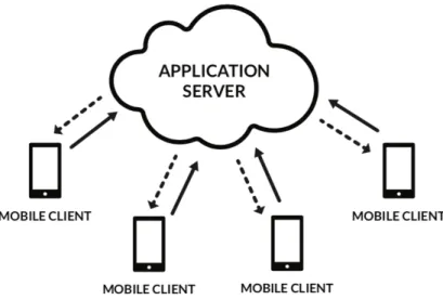
Figure 2.1: General Mobile Crowd Sensing Architecture
As coordinated distributed software platforms, Mobile Crowd-sensing systems are usually composed of a central in-cloud application server and several mobile clients. The central server is responsible for managing all the centralised phases of the whole sensing and processing procedure.
It implicitly or explicitly assigns the sensing tasks to the users and then receives data collected by participants. The sensing task is performed in a decentralised manner through mobile clients of volunteers. The software client can collect data directly or with the help of the user. For a more comprehensive analysis of typical MCS architectures, see the work of Louta et al. [13].
2.4
Libraries and Tools
The project as described needs suitable tools and procedures for the analysis and extraction of information. The database contains millions of records and this number is going to grow exponentially in the future.
2.4.1
Jupyter and Python
The main tools used are Jupyter Notebook (version 4.4.0) and Python (version 2.7 in this work). The Python version is fundamental for the PySpark environment used locally on the machine when experimenting.
2.4. Libraries and Tools 11
2.4.2
Apache Spark
Spark is a unified analytics engine for large-scale data processing created by Apache to distribute the workload on clusters. It provides high-level APIs with which to develop the applications to be submitted to Its cluster manager that takes care about the processing involved.
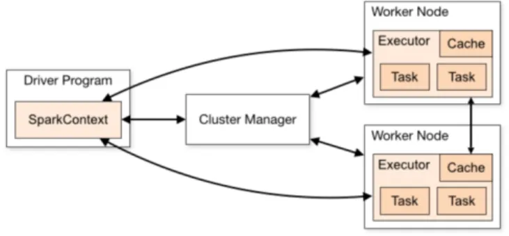
Spark applications run as independent sets of processes on a cluster, coordi-nated by the SparkContext object in the main program (called the driver program). Specifically, to run on a cluster, the SparkContext can connect to several types of cluster managers (either Sparks own standalone cluster manager: Mesos or YARN), which allocate resources across applications.
Once connected:
1. Spark acquires executors on nodes in the cluster, which are processes that run computations and store data for the application;
2. It sends the application code (Python for this work) to the executors; 3. The SparkContext sends tasks to the executors to run.
Figure 2.2: Spark Job Flow
There are several things to note:
1. Each application gets its own executor processes, which stay up for the du-ration of the whole application and run tasks in multiple threads.
• PRO: The applications are isolated each other: on both the scheduling side (each driver schedules its own tasks) and executor side (tasks from different applications run in different JVMs).
• CONS: Data cannot be shared across different Spark applications (in-stances of SparkContext) without writing it to an external storage sys-tem.
2. Spark is agnostic to the underlying cluster manager. As long as it can acquire executor processes, and these communicate with each other, It is relatively easy to run It even on a cluster manager that also supports other applications (e.g. Mesos/YARN).
3. The driver program must listen for and accept incoming connections from its executors throughout its lifetime. As such, the driver program must be network addressable from the worker nodes. Because the driver schedules tasks on the cluster, It should be run close to the worker nodes, preferably on the same local area network.
Resilient Distributed Dataset
Spark revolves around the concept of a Resilient Distributed Dataset (RDD), which is a fault-tolerant collection of elements that can be operated on in parallel. Parallel collections are created by calling sc.parallelize() method on an existing collection in the driver program. The elements of the collection are copied to form a distributed dataset that can be operated on in parallel.
One important parameter for parallel collections is the number of partitions to cut the dataset into. Spark will run one task for each partition of the cluster. Typically, Spark tries to set the number of partitions automatically based on the cluster properties. However, It is possible to manually pass the number of parti-tions as a second parameter to the parallelize() method.
RDDs support two types of operations:
1. Transformations: which create a new RDD from an existing one;
2. Actions: which return a value to the driver program after running all the transformations on the RDD.
For example, map is a transformation that passes each RDD element through a function and returns a new RDD representing the results. On the other hand, reduce is an action that aggregates all the elements of the RDD using some func-tion and returns the final result to the driver program.
All transformations in Spark are lazy, in that they do not compute their results right away. The transformations are only computed when an action requires a re-sult to be returned to the driver program. This design enables Spark to run more efficiently. For example, we can realise that a RDD created through map will be used in a reduce and return only the result of the reduce to the driver, rather than the larger mapped RDD.
By default, each transformed RDD may be recomputed each time an action is performed. However, persisting the RDD in memory using persist() or cache() method allow to keep the elements around on the cluster for a much faster access.
2.4.3
Google Cloud Platform
Massively parallel processing using tools such as Spark can be performed locally for small data sets and Its local implementation can be used to perform
optimisa-2.4. Libraries and Tools 13
tion operations before proceeding to launch a specific algorithm on a cluster. If the operations to be performed require clusters with non-negligible resources and not negligible execution times, then locally studying an algorithm should be exploited in this sense.
Google offers a service called DataProc that allows the creation of tailor-made clusters on demand. The service is obviously not free but excellent in all cases It is necessary to perform tasks with tools such as Spark. However, It is very cheap and has been used to pre-process the SmartRoadSense data set.
2.4.4
QGIS
Quantum GIS (QGIS) is an open source GIS desktop application, very similar in user interface and functions to equivalent commercial GIS packages.
The use of QGIS is related to the generation of borders (namely in shapefiles) used to apply the geo-spatial queries to the areas on which the analysis has been performed.
Chapter 3
Related Works
3.1
Mobile Crowdsensing Applications
3.1.1
Data Collection and Processing Workflow
Figure 3.1: MCS Application Workflow
The Mobile Crowd-sensing applications follow a general pattern before coming on the market. There are several definition like the one below, that It is considered the most accepted one with some original change. The workflow is based on the proposal of Dr. Saverio Delpriori [15], shown in Figure 3.1.
Task Creation
In this first phase, the central entity creates specific tasks and provides a de-tailed description of the required actions. The task creation can be even started by users, the same ones who will consume the data collected using the Mobile Crowd-sensing application.
Depending on the platform used, the description could be either in natural language or domain specific language that software clients are able to understand and present to volunteers. In some cases, the task creation is implicit in the platform structure. Volunteers who join the application are automatically tasked with a defined sensing operation [14].
Task Allocation
The central entity can analyse the sensing task and assign it to specific partici-pants (or nodes of the sensing network) possibly trying to respect given constraints: ensuring area coverage, minimising the task completion estimated time, maintain-ing the number of volunteers involved under a given threshold, ensurmaintain-ing a minimal average trust value among the selected participants, and so on.
Another approach is to notify all clients that a new task is available and let them choose whether to take part in the sensing task or not. Depending on the mo-tivation incentive systems utilised, some systems also allow approaches like auction based assignments.
Data Sensing
Involves both information sensed from mobile devices and user contributed data from mobile internet applications. MCS applications usually have to tackle secu-rity and privacy issues, thus providing users with automated or semi-automated mechanisms determining what kind of information they want to publish and whom to share them with is fundamental.
Many MCS systems resort to access control mechanisms and pre-anonymisation techniques. In order to reduce transmission costs and size, data is often pre-processed on board of the user device. Finding the appropriate trade-off between the amount of processing to be done onboard of smartphones and in cloud after the data has been transmitted is a crucial parameter for a MCS application.
Data Collection
In this phase, data is received by mobile clients and stored into appropriate memory supports. Privacy-preserving techniques are applied to ensure security and to avoid that malicious users acquire collected data and can track them back to users. The sensor gateway module provides a standard approach - usually im-plementing common web services technologies - to enable data collection from
3.1. Mobile Crowdsensing Applications 17
crowd-sensed sources supplying a unified interface.
MCS applications may collect a vast amount of heterogeneous data and big data storage systems are usually employed. Big data techniques simplify the col-lection of large-scale and complex data like noise level measured across an urban area. Sensing tools used by participants to evaluate the phenomenon at stance typ-ically varies a lot, leading to significant differences in the accuracy of crowd-sensed data. Therefore, data is commonly transformed and unified before being stored and passed to the next phase in order to boost further processing.
Data Processing
Aims to derive high-level intelligence from raw data received. Using logic-based inference rules and machine-learning techniques this step focuses on discovering fre-quent data patterns in order to extract crowd-intelligence starting from data sensed by mobile users and user-contributed data from other mobile internet applications mixed together.
The first step of the data processing is the data aggregation phase, in that, raw data from different users, time and space are combined on different dimensions and associated with reference known features (e.g., map-matching [16]).
Then further data processing techniques are applied to extract the three kinds of crowd-intelligence (namely: user awareness, ambient awareness, and social aware-ness). When information passes through this phase, different statistic methods are applied to classify the quality of processed data.
Data Distribution
Once data have been aggregated, and the crowd-intelligence has been extracted from them, this information is usually made publicly available to be re-used (often as Open Data) or only shared in a private way with authorities, communities, companies, etc.
Exploitation
Finally data arrive at the stage where they are re-used, exploited or just shown. The implementation of a usable user interface and of data visualisation techniques (such as mapping, graphing, animation) are essential to fully exploit the
crowd-intelligence extracted by the underlying system starting from raw data.
Cooperation Incentives
As shown in Figure 3.1, the cooperation incentives phase influences almost every other stage of the proposed framework. Users can be motivated to participate in a sensing task by using incentives in the task allocation phase. In the sensing phase,
the idea of a possible future reward can motivate users to collect better or more data.
3.1.2
Real-World Applications
Mobile Crowd-sensing applications can serve as sensing and processing instru-ments in many different fields. Due to mobile devices inherent mobility, they can be utilised for sensing tasks aimed to gain better awareness and understanding of urban dynamics. Acquiring knowledge in such context is of prime importance in order to foster sustainable urban development and to improve citizens life quality in terms of comfort, safety, convenience, security, and awareness.
Many other studies have investigated urban social structures and events start-ing from crowd-sensed data. Crooks et al. studied the potential of Twitter as a distributed sensor system. They explored the spatial and temporal characteristics of Twitter feed activity responding to a strong earthquake, finding a way to identify impact areas where population has suffered major issues [17].
Large-scale data can be also collected by means of MCS platforms to analyse the actual social function of urban regions, a kind of data which is usually very difficult to obtain and that can be of primary importance concerning urban plan-ning. For instance, Pan et al. started from the GPS log of taxi cabs to classify the social functions of urban land [18], while Karamshuk et al. tried to identify optimal placements for new retail stores [19].
Awareness of user location is the foundation of many modern and popular mobile applications, such as location search services, indoor positioning, location based-advertising, and so forth. But more useful and precise services can be en-abled harnessing all the peculiar characteristics of personal mobile phones. As an example, Zheng et al. used crowdsourced user-location histories to build a map of points of interest which can be of help for people who are familiarising with a new city [20].
Other cases are Geo-Life [22], a Mobile Crowd-sensing platform able to suggest new friendship looking at similarities in user-location logs. Or CrowdSense@Place [24], a framework able to exploit advanced sensing features of smartphones to op-portunistically capture images and audio clips to better categorise places the user visits.
In many cases, the development of a particular platform has been the answer to issues raised by pre-existing communities or grassroots initiatives. Citizens and policy makers have usually strong interests in matters like environmental monitor-ing, public safety and healthcare, where the participatory and mobile essence of the Mobile Crowd-sensing approach provides a novel way for collaboratively monitor the issue being considered.
3.1. Mobile Crowdsensing Applications 19
3.1.2.1 Crowdsensing for the common interest
The moving nature of these topics draws the attention of online and offline communities. The potential of a community can be harnessed by MCS approaches to engage people and to make them participate in the data collection. It is not just a matter of the number of participants, rather someone who is moved by a topic not only will be more disposed to contribute but will also be prone to provide better and more complete data.
As an example, Ruge et al. described how their application SoundOfTheCity [25] allowed users to link their feelings and experiences with the measured noise level, helping in providing information essential to have a more clear understanding of the context (is the high noise level in a party, at a festival or just in a crowded street?). This is an illustrative case of how qualitative data provided by users can enrich the quantitative data gathered through personal smart devices.
In short, to fully harness their potentialities when analysing such contexts, MCS applications should aim not only to collect as much data as possible but also to provide ways for users to enrich the collection with thick data.
Then there are other examples of MCS applications analysing topics of common interest as:
• NoiseTube [26] which was a system able to exploit volunteers smartphones to collect data about environmental noise in users daily lives and to aggregate them to obtain a fine-grained noise map;
• U-Air [23] inferred air quality data by heterogeneous crowd-sensed data comparing them against information from sensing stations and traffic infor-mation.
Healthcare is another field where MCS is helping a lot by collecting a wealth of data for applications more and more useful for an ageing society like ours. Google researchers did pioneering work in 2006 using health-related search queries to es-timate illnesses distribution in US [27], while Wesolowski et al. exploited the widespread diffusion of mobile phones to analyze malaria spreading in Kenya [28].
3.1.2.2 SmartRoadSense
An application only based on data sensed using personal user smartphone is SmartRoadSense [14]. The platform is a crowd-sensing system used to monitor the surface status of the road network. The SmartRoadSense mobile app is able to detect and classify the road surface irregularities by means of accelerometers and send them to an in-cloud server. Aggregated data about road roughness are shown on an interactive online map and made available as open data1.
Figure 3.2: SmartRoadSense Process Flow
The system has been developed to provide quantitative estimations of road net-work surface roughness. The approach at data sensing and processing is general enough to be employed also in different contexts. As many other MCS platform, sensing tasks in SmartRoadSense are performed by multiple distributed sensing devices by means of which volunteers contribute to gauge the quantity of interest in a specific location, within a specific time-window.
As shown in Figure 3.2, the architecture of the SmartRoadSense platform is characterised by the following three layers:
• Mobile Application: An app running on users smartphones during a given car trip. The application makes use of the smartphones accelerometers and computation capabilities to collect and process acceleration values the device is subject to. The result, representing the estimated roughness of the trav-elled road in a given point at a given time, is geo-referenced, time-stamped, and transmitted to a server by means of radio connectivity.
• Cloud Platform: A cloud-based back-end service in charge of collecting, aggregating and storing data from multiple users. The platform is in charge of two tasks:
– MapMatching: geo-referenced roughness indexes stored in the database of raw-data (SRS_RAW) are projected on digital cartography maps, specifically OpenStreetMap. Map-matching entails the association of GPS points to features on a digital cartography maps.
– Sampling and Aggregation: data is subsequently aggregated to pro-vide a single evaluation (for a given spatial coordinate) of the rough-ness index, given the data made available for that point by multiple users. Aggregated data is used to populate the related database (called SRS_AGGREGATE).
3.1. Mobile Crowdsensing Applications 21 • Visualisation: A front-end service providing visualisation capabilities of the geospatial information produced by the SmartRoadSense processing pipeline. The same front-end also allows interested end-users to download a continu-ously updated version of the database containing all SmartRoadSense aggre-gated data in a ready-to-be-reused fashion (the schema of the table is visible in Table 3.1). Each row of the open-data dataset contains a set of informa-tion relative to the roughness level, the geo-localisainforma-tion, the quality of the data, and even a indication of the estimated number of occupants of each vehicle that has been involved in the gathering process.
COLUMN FORMAT DESCRIPTION
LATITUDE DECIMAL DEGREES The latitude coordinate of center of the section of the road where the PPE value has been estimated LONGITUDE DECIMAL DEGREES The longitude coordinate of
cen-ter of the section of the road where the PPE value has been es-timated
PPE DECIMAL The average roughness level of the
road section
OSM_ID LONG INT The ID of the road in the
Open-StreetMap
HIGHWAY TEXT The road category according
to the OpenStreetMap classifica-tion2
QUALITY DECIMAL A numerical estimate of the qual-ity of this particular PPE value. This quality index has been calcu-lated using our bootstrap-based method, in our case-of-study PASSENGERS DECIMAL The average of the number of
pas-sengers in vehicles involved in the process
UPDATED_AT DATE (ISO 8601) The last update of the data for that particular road section
Table 3.1: SmartRoadSense Open Data Schema
In SmartRoadSense (and possibly in other MCS Systems), the sensing process can be divided into time epochs, during which data is continuously gathered, pro-cessed and aggregated. At the end of a given time epoch the system updates current information on the status of measured variables and, in case, It performs a composition operation with data collected in previous epochs (in SmartRoadSense
an epoch represents a week of monitoring activity).
The platform continuously receives values of road roughness from end users. Roads are spatially segmented into landmark points, then all values associated to positions falling within a given range (typically 20 meters) of a landmark point p are aggregated and concur to the overall roughness index of p (the mean value of contributed points is taken by default). At the end of each week current epoch ter-minates, and the roughness value of each point p is updated by taking the average between the value of current epoch and the value of previous epoch.
This processing inherently implements a form of infinite impulse response filter, the aim of which is to progressively down-weigh (through an exponential decay of weights) the contribution of older samples to the value assigned to p.
Chapter 4
The General Approach for Value
Identification
As mentioned in the previous chapter, a data set is considered “Big Data” if It satisfies the properties of: volume, variety and velocity.
However, data alone is not enough. Evaluating Its veracity is needed in order to understand if It can be useful to exploit. To explore this property a specific roadmap has been followed and the concept of value has been defined.
4.1
The Concept of Value
What is value in Big Data? As seen in Chapter 2, the word of value is included in the concept of veracity. But what really mean value for the data? In this case there is no real definition.
If the meaning of value is referable to an economic concept and therefore to an intrinsic property of an object, such as the currency, then the quantity would determine the amount of value held and the greater the coins owned, the greater is the value. Then we could converge on the same idea: a large amount of data represents a great value. However, some could argue: for the same amount of coins held, the one that owns more value is the one who possess those with the higher intrinsic value. But a third party intervenes and claims that It is the market that gives value to the currency and since some currencies have greater market value, in the end the one who has more value is who possesses the higher amount of coins with the greater intrinsic value and market value.
The problem is therefore to ask if the datum represents an intrinsic value: my answer is no. If the datum represented an intrinsic value then we should not verify information or quality of the data, as this property would be intrinsic to the infor-mation itself. But in fact, this is not the case for data, which in no way represents an immutable concept. The data is basically a raw material that needs to be pro-cessed to generate value.
Therefore, It is not enough to say that: the data acquire value if they are in a big amount. The value is determined by indicators, even multiple, which we could define as metrics, that if crossed together can generate the notion of value. For example, the value in the case of geospatial data could be determined by the fact that they must be in large quantities and be recent. However, this statement is strongly dependent on the goal of data handlers. To conclude, by value of the data we mean the goal generated by the data after a regulated evaluation respecting specific indicators, called metrics.
4.2
The Proposed Approach
When looking to geospatial data It is interesting to know which records would be used for exploitation (i.e. researches).
In big data sets as geospatial ones, It is a challenge to realise which records are useful for this purpose. The data may present several complications:
• Size: disk space can be large to the order of gigabytes or terabytes;
• Volume: the amount and the complexity of records may be high and the greater the complexity, the greater the computational cost required to process a record;
• Velocity: the records could be updated frequently;
• Sparsity: the geospatial points could not be distributed equally on time and space so, It is difficult to have enough information regarding the terri-tory analysed, despite the high volume.
To this end it makes sense to implement an approach developed in different phases, in order to define a process that suggests the correct analysis of geospatial data sets. The process thought is based on 5 main phases:
1. Exploratory Analysis: a very first analysis to obtain more information about the data set considered;
2. Outcome Definition: the definition of the metrics used to give the defini-tion of value;
3. Pre Processing: reducing data set volume avoiding redundancies; 4. Processing: using the different metrics to generate results;
4.3. Exploratory Analysis 25
4.3
Exploratory Analysis
Exploratory analysis is the very first phase to face when having an unknown data set. In this phase It is necessary to take into consideration the shape char-acteristics of the data set such as its weight and the volume in terms of records, trying to get a comprehensive idea of the data set itself and its critical issues.
4.3.1
Data set
A data set could be structured or unstructured but reducible as a set of rows and column. Analysing a data set means mainly understanding its shape character-istics, i.e. the size, the number of records contained and the amount of information per record. This last point is particularly important since the number of columns generated impacts on the computational complexity and memory occupation. For this reason, this phase focus on carry out a quantitative analysis of the data set that allows to anticipate the dimensions in RAM.
The RAM memory occupancy estimate in Python can be easily performed by having a single data set record available, appropriately transformed according to the criterion that will be used during the Pre-Processing phase. This is because the information that you want to get from the single record is its memory occupa-tion and therefore It is necessary that the record is formatted exactly as It will be. The second information concerns instead the number of rows contained in the data set, information obtainable through the Unix terminal, through Spark or the I/O methods available in Python. At this stage It is clear that the data set should only be read, any attempt to load a data set of the Big Data order into memory will saturate the RAM available on the machine, making the application unresponsive. The estimate can then be reduced to:
memory occupancy∗ number of lines
To be more detailed about the methods that can be used to derive this information is good to cite:
• UNIX: wc -l <dataset.extension> • Spark: count() method
• Python: Read and Write operations on files
4.3.2
Insights
Once that the data set form is clear, It is necessary to understand the distri-butions of data over space and time. Geo-spatial data sets contain millions of records that are potentially distributed throughout the world. This last assump-tion directly refers to what had been introduced in the previous chapters: in such
a large context of data collection such as geo-spatial data, the risk of not having enough data to be able to generate value is very high and strongly dependent on the problem considered. As anticipated, It is not enough to know quantitatively the distribution of data on the territory to understand Its value because quantity alone is not synonymous of value. The data must be interpreted according to the context in which they are considered.
The exploration is therefore very important at least to understand the obsta-cles that stand in the ability to generate the value from data, quantifying them qualitatively. For example, in Figure 4.1 a road for which the data collected over time have been obtained (many similar ones have been found). It is clear that for the SmartRoadSense data set there is a problem of fair distribution over time and space, perhaps due to the youth of the application, which in any case hinders the achievement of value.
Figure 4.1: Example of bad data collection
4.4
Outcome Definition
After obtaining the insights regarding the data set, It is time to define the goal to achieve, that is the metrics that will be used to define the value.
The idea is that since geospatial data sets could show the previous deficiencies, the focus should be on appropriate metrics that together can generate results that can be crossed together in order to highlight which records can be more promising for one’s needs.
The goal should be focused on using metrics that are meaningful for the work considered. One could search for the amount of data in a territory, their degree of topicality, the trend over time of the recordings and so on. Other metrics can be freely added or the previous proposals can be removed if not useful.
4.5. Pre Processing 27
These tasks could then be converged into a single solution that can fully describe the data considered, allowing a correct final big picture retailed on its own definition of value.
4.5
Pre Processing
The Pre Processing part is essential for the final solution. Once the metrics are settled, with all probability a large part of the available data will not be useful for solving the problem because they simply represents redundancy.
For this phase, Spark tool is available but in order to perform data Pre-Processing, lots of companies use other solutions like UNIX, perhaps coupled with incremental loading. But many tools are available: Python, or the same SQL could help.
However, these approaches vary from problem to problem and are not always applicable especially with geospatial data, for example:
• Using SQL assumes that a distributed database in which the data is stored is available, such as PostGIS. Instead, often geo-spatial data is provided as Open Data in text files.
• Using SQL assumes that any geospatial operations are procedures within the database, limiting the freedom that a programming language like Python offers.
• Using the UNIX console for non-trivial operations such as a spatial query is not a valid alternative to Spark in addition to introducing perhaps greater restrictions than those offered by SQL with a distributed geospatial database.
Spark’s success is therefore guaranteed because of the convenience It represents: its instruments have a great usability and are much more extensive. Despite not finding a real application in local, their use in limited available hardware allows a better settings of the algorithms developed with it.
In fact, the Pre Processing phase if done locally allows to put in place all the necessary tools in the absence of resources, allowing to not worry about the re-sources available in the code writing and optimisation phase.
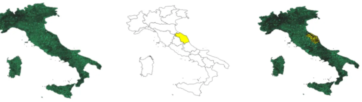
Moreover, the Pre Processing phase in the case of geospatial data involves not only the removal of redundancies but also a multitude of other operations such as spatial functions. Spatial functions, or called spatial queries, are useful methods for selecting records on a territorial basis. Through Python It is possible to perform them and with Spark It is possible to develop an algorithm that can exploit the maximum parallelism to execute them. An example of a spatial query application is shown in Figure 4.2 where all the municipalities have been selected across the borders of the Marche Region.
Figure 4.2: Municipalities Selected through Spatial Query in QGIS
If you imagine that this kind of operations should be performed for every single record of the geospatial data set, the complexity of the problem tends to explode. To this end, in this phase the optimisation is fundamental for a subsequent imple-mentation on clusters with the precise objective of providing the results in a short time, since It makes sense to obtain results in a short time in a real-time context. For the implementation of clusters there are several providers available, for example Amazon, Google and Microsoft. For the project Google DataProc was used for convenience but any other solution is certainly valid.
4.6
Processing
At the end of the Pre-Processing phase a new data set is produced which is almost free of redundancies and tailored in respect of the goal, therefore containing the information necessary for the implementation of the metrics.
In this phase the defined metrics are implemented and subsequently crossed together to form the final data set which should be a correct summary of the three. Python in this case lends itself very well to the purpose, allowing data manipula-tion, which this time is no longer of unmanageable volumes.
However, before generating the results It is necessary to carry out a further operation that can guarantee the quality of the data set generated in the Pre Pro-cessing phase. In particular, in the specific case of SmartRoadSense, but this may happen for any data set, the anomalies may have been easily introduced for some reason. Before generating the results of the predefined metrics It is therefore nec-essary to verify that the data set produced is free of anomalies, or that the new distributions generated contain data that are consistent with one another.
As an example, once the Pre Processing operation was performed on the SmartRoad-Sense data set and the new data set was generated with the necessary information for the metrics, It was noticed that many distributions presented data far outside
4.7. Visualisation 29
the average, such as in Figure 4.3. Their removal is therefore necessary before proceeding.
Figure 4.3: Example of Anomalies in a Time Series
Finally, It is possible to proceed doing the operations that aggregate the data to obtain the values for the necessary metric. Once crossed, the results are ready to be shown.
4.7
Visualisation
Figure 4.4: Example of Visualisation with Plotly
The visualisation consists in giving a final picture of the results obtained in the Processing phase. On the basis of the Processing phase, It makes sense to visualise the generated results for immediate understanding.
The tools useful for visualisation are many: It is possible to use web apps, mo-bile applications, libraries available in different languages. The criterion is free but has the common objective of forming an overview of rapid comprehension.
In this work the plotly library available in Python was used for convenience, which allows the overlapping of several layers and the insertion of legends and captions as in Figure 4.4
Chapter 5
Implementation Experience
The implementation is based on the process defined in the previous chapter. The meaning in terms of implementation is illustrated in the next sections, point by point. To develop the final solution the Spark environment has been used locally, the drawbacks related to this choice are discussed later on Chapter 6, as well as the solutions to them (the use of a cluster). This evidences of this is not discussed in this chapter since the algorithm written with Spark (locally) can be ported on a cluster with little efforts.
To sum up, the approach for identifying the value in geospatial data sets is as follows: 1. Exploratory Analysis 2. Outcome Definition 3. Pre Processing 4. Processing 5. Visualisation
5.1
Exploratory Analysis
In the very first part of the process a qualitative analysis of the data is car-ried out which led to the formulation of several important considerations for the development of the final solution.
5.1.1
Data set
The data set available comes from a PostGIS database of hundreds of millions records. SmartRoadSense is built on two different databases:
• Raw Database: It contains the measurements coming from the mobile application that runs on mobile devices. This data is stored for its future aggregation.
• Aggregate Database: It contains data generated starting from raw data. It is weekly generated for each road throughout the year.
The data considered is part of the Italian peninsula, country (together with the United Kingdom) from which the pilot of the project started, therefore at least theoretically more populated of information. As a local area for showing the process an even smaller area has been focused (the Marche region) for three main reasons:
• The project started at the University of Urbino, whose municipality resides in the Marche region
• The approach generated must be scalable regardless of the volume of data
5.1.2
Row Attributes
A typical row of the SmartRoadSense dataset contains the following information (only the significant ones will be cited):
• single_data_id: Unique ID of the measurement; • date: Time Instant of Sampling;
• osm_line_id: OpenStreetMap ID; • ppe: Deterioration Value;
• speed: Vehicle Instantaneous Speed;
• position: The projection of “Position” on the relative road;
• track: The track that registered the information (available only for raw data).
The following attributes: osm_line_id, position, track play an important role in the analysis because they constitute three different concepts:
• Section: a section is identified through its osm_line_id, the id through which OpenStreetMap identifies a section of a road in its global map. In other words, for each road of any length, OpenStreetMap maps portions of this street within its dataset by associating a given ID. Consequently, a real road is often composed of several sections.
• Segment: a segment is identified by the position attribute. Within a section, many segments of a length of twenty meters are identified, therefore the number of segments contained in a section will be equal to the ratio between the length of the section in meters and the length of the segment.
5.1. Exploratory Analysis 33 • Track: when a user collects data He produces a track. A track can involve several roads, as well as several section. This information is only available for raw data, when the data is collected. This means that when a user travels on some road, an identifier is marking his trip.
5.1.3
Retrieving Informations
A Spark environment was used on the local machine for exploring the data set. The SmartRoadSense data set of the Italian peninsula alone contains about 20 million records and a number of columns for each row equal to 16. Through the code in Listing 5.1 it was possible to estimate the amount of memory needed to load the entire data set in RAM. The result is just over 20 GB of RAM.
1 data = sc . t e x t F i l e (’ ../ D a t a s e t s / E x t r a c t i o n 10/ r a w _ i t a l y .
csv ’) \
2 .map(l a m b d a line : line . e n c o d e (’ a s c i i ’, ’ i g n o r e ’
) )
3
4 c l e a n = data .f i l t e r(l a m b d a row : row != h e a d e r . v a l u e ) \ 5 .map(l a m b d a row : re . sub (r ’ \{[\ s \ S ]*\} ’, ’ {} ’
, row ) ) \
6 .map(l a m b d a row : row . s p l i t (" , ") ) \
7 .map(l a m b d a row : row [ : 4 ] + [ c o n v e r t _ d a t e ( row [4]) ]+ row [ 5 : ] )
8
9 p r i n t sys . g e t s i z e o f ( c l e a n . take (1) ) * 2 0 0 0 0 0 0 0
Listing 5.1: Evaluating RAM Occupation
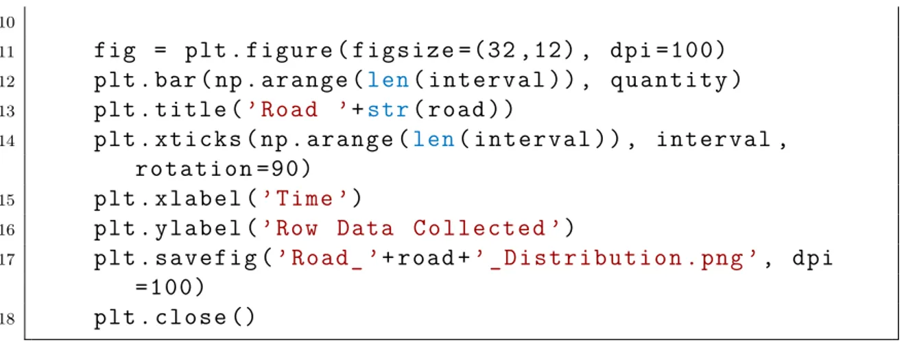
Subsequently, the exploration continued extracting data step-by-step, develop-ing an algorithm to plot results avoiddevelop-ing to load the whole amount in memory. The algorithm developed on Spark, although poorly performing due to local operation, was pretty useful for plotting without the risk of having the RAM saturated. The code is visible on Listing 5.2.
1 % m a t p l o t l i b i n l i n e 2 i m p o r t os 3 for road in u n i q u e _ r o a d s : 4 q u a n t i t y = [] 5 for elem in tqdm ( i n t e r v a l ) : 6 c o u n t = r d d _ p l o t .f i l t e r(l a m b d a row : row [0] == road ) \ 7 .f i l t e r(l a m b d a row : row [1] <= elem and row [1] > elem -d a t e t i m e . t i m e -d e l t a ( -days =7) ) \
8 . c o u n t ()
10 11 fig = plt . f i g u r e ( f i g s i z e =(32 ,12) , dpi = 1 0 0 ) 12 plt . bar ( np . a r a n g e (len( i n t e r v a l ) ) , q u a n t i t y ) 13 plt . t i t l e (’ Road ’+str( road ) ) 14 plt . x t i c k s ( np . a r a n g e (len( i n t e r v a l ) ) , interval , r o t a t i o n =90) 15 plt . x l a b e l (’ Time ’) 16 plt . y l a b e l (’ Row Data C o l l e c t e d ’) 17 plt . s a v e f i g (’ R o a d _ ’+ road +’ _ D i s t r i b u t i o n . png ’, dpi = 1 0 0 ) 18 plt . c l o s e ()
Listing 5.2: Plotting exploration’s results
5.1.4
Insights
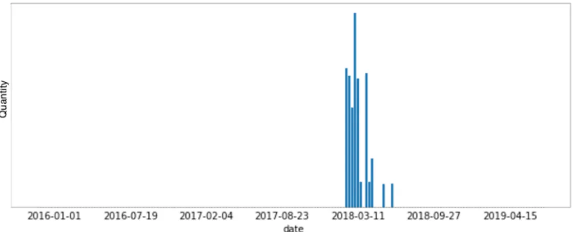
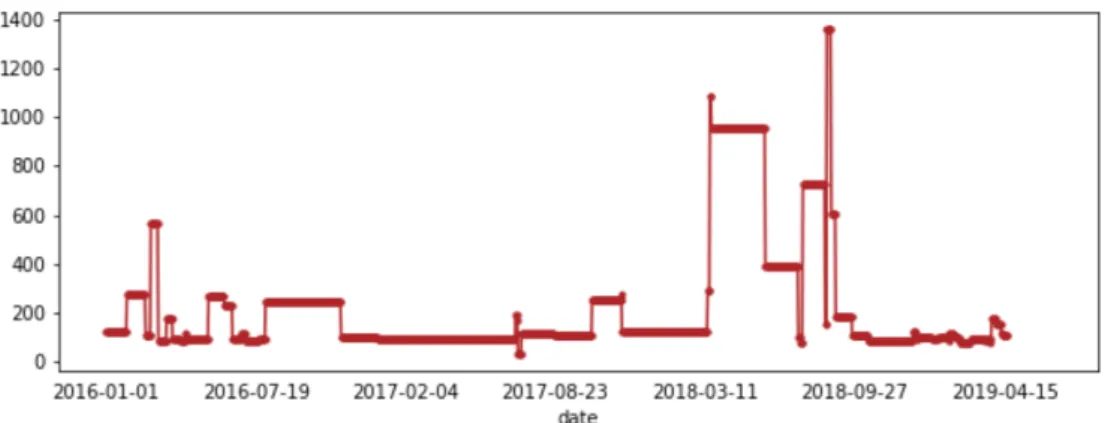
What came out analysing the the plots generated is that the data is still too few and scattered even when decreasing the granularity. For example, in Figure 5.2 the granularity is totally reduced: It only shows the quantities of measurements collected over time from the first moment the SmartRoadSense platform was acti-vated (2016) for a certain road. By a quick look of the graph It is clear that the available window of data is too small (18 weeks, more or less 3 months). This plot has been generated by taking the twenty most travelled roads, i.e. those with the greatest number of measurements.
Figure 5.1: Measurements distribution for road 97464677
So, if the latter case was incomplete, trying to increase the granularity looking to each section of one road is useless. Suppose that for a future research we should be able to guess the speed of deterioration or predict when a certain section will deteriorate: with the available data this forecast is not possible even by using fill-ing techniques that can make the time series complete. There is simply no data to generate value regarding that road.