Comparison of concept drift detectors in a health-care facility dataset to detect behavioral drifts

(1)

Politecnico di Milano Scuola di Ingegneria dell’Informazione

Polo territoriale di Como Master of Science in Computer Engineering

Comparison of Concept Drift Detectors in

a Health-Care Facility Dataset to detect

Behavioral Drifts

Supervisor: Prof. Sara Comai

Assistant Supervisor: Eng. Andrea Masciadri

Master Graduation Thesis by: Fabio Masciopinto Student Id. number: 899148

(2)

(3)

All’amicizia, senza la quale, non avrei potuto realizzare

(4)

(5)

Sommario

Questa ricerca descrive gli algoritmi che analizzano stream di dati in evoluzione con lo scopo ultimo di apprendere da essi in tempo reale avvalendosi dell’utilizzo del framework MOA, uno tra i più popolari open source framework progettato per l’implementazione di quest’ultimi. L’obiettivo della tesi è quello di testare gli algo-ritmi di concept drift detector implementati nel framework andando ad analizzare le Activities Daily Livings (ADL) umane per prevedere e controllare le malattie, soprat-tutto mentali, che sono causate dall’avanzamento d’età degli individui. In letteratura, in riferimento a questo argomento, molti autori pongono la loro attenzione allimpor-tanza di monitorare il comportamento di un individuo in relazione al suo benessere dando però meno importanza ai cambiamenti comportamentali individuati dallo stu-dio dei dati prodotti da dispositivi tecnologici quali possono essere i sensori. Questo studio inizia con l’analisi delle prestazioni dei rilevatori di concept drift in MOA su dati generati da quest’ultimo tramite specifiche opzioni implementate nel framework. Gli stessi, poi, sono stati testati su un dataset che simula il comportamento degli individui in diverse attività quotidiane (ADL) contenti in maniera artificiale diversi tipi di drift. In seguito, sono stati fatti diversi esperimenti con diverse configurazioni per rilevare i miglior detection learner in base alle diverse tipologie di drift. I risul-tati degli esperimenti rivelano che i drift di tipo Abrupt possono essere facilmente rilevati attraverso il metodo DDM o più in generale con un algoritmo basato sulla statistica. Tramite l’EDDM è invece possibile trovare in modo molto dettagliato la i drift di tipo Gradual. Infine, per quanto riguarda gli Incremental drift, possiamo usare il metodo ADWIN che è in grado di identificare le varie derive comportamentali riguardo andamenti incrementali nel tempo ma, in presenza di rumori, periodicità e anomalie, questo metodo non è raccomandato. In questi casi, infatti, potrebbe essere megli utilizzare l’algoritmo SEED Change Detector che sfrutta la sua componente di statistica pure essendo un metodo basato sulle finestre.

(6)

(7)

Abstract

This research describes the algorithms that analyze evolving data streams with the ultimate aim of learning from them in real-time using the MOA framework, one of the most popular open-source frameworks designed for the implementation of the latter. The objective of the thesis is to test the concept drift detector algorithms implemented in the framework by analyzing human Activities Daily Livings (ADL) to predict and control diseases, especially mental ones, that are caused by the advancement of individuals by age. In literature, about this topic, many authors focus their attention on the importance of monitoring the behavior of an individual concerning his well-being, while giving less importance to the behavioral changes identified by the study of data produced by technological devices such as sensors. This study begins with the analysis of the performance of concept detectors drift in MOA on data generated by the latter through specific options implemented in the framework. The same, then, were tested on a dataset that simulates the behavior of individuals in different daily activities (ADL) artificially containing different types of drift. Later, several experiments were made with different configurations to detect the best detection learner based on the different types of drift. The results of the experiments reveal that Abrupt drifts can be easily detected through the DDM method or more in general with an algorithm that is statistically based. Through the EDDM it is possible instead to find in a very detailed way Gradual drift. Finally, as far as the incremental drift is concerned, we can use ADWIN able to identify all the various behavioral drift over time but, in the presence of rumours, periodicity and glitches, this method is not recommended. In these cases, in fact, could better use a SEED Change detector algorithm that exploits its statistic component even being a window based method.

(8)

(9)

Ringraziamenti

Desidero innanzitutto ringraziare la Professoressa Sara Comai e Andrea Masciadri per la disponibilit`a e la pazienza che hanno avuto nei miei confronti, per la costante presenza e il grande aiuto che mi hanno dato nel mio lavoro.

Ringrazio i miei genitori che mi hanno sempre supportato in questo lungo cammino senza mai farmi mancare nulla. A voi devo quello che sono oggi, e quello che un giorno vorr`o diventare. Grazie per tutti i sacrifici che avete fatto per rendere questo momento possibile. Spero di avervi reso orgogliosi di vostro figlio.

Ringrazio mia sorella, Laura, la prima a credere nelle mie potenzialità e a sp-ingermi ad affrontare questo percorso. Senza di lei ora sarei ancora in un ufficio a compilare scartoffie. Non c’è attimo in cui non sento la sua fiducia. Grazie per avere sempre un pensiero rivolto verso di me. Se un domani sarò qualcuno , lo devo soprattutto a te, non me lo scorderò.

Anche se implicitamente la ringrazio tutti i giorni, un grazie doveroso va a colei che mi supporta, ma più che altro mi sopporta. Alla mia vecchia preferita, alla mia complice di vita, alla mia ragazza ma più semplicemente alla mia Lele, la Donna che sono orgoglioso di avere al mio fianco. Mi sei sempre stata vicino nei momenti difficili, sia della mia carrriera universitaria che della mia vita. Non mi hai mai abbandonato anche quando avresti avuto tutti i motivi per farlo. Grazie per essermi stata vicino nei miei scleri giornalieri e di aver alleviato le mie ansie pre e post esami. A te devo la mia felicità. Grazie. Ti Amo.

Il mio grazie pi`u grande va al mio migliore amico, Gigi. Anche se non te l’ho mai detto prima, tu hai avuto un ruolo fondamentale per me. Sapere che ci sei sempre e comunque nella mia vita mi ha aiutato tanto, soprattutto nei primi anni qui a Como. Tu mi hai insegnato a lottare e non arrendermi mai, mi hai insegnato a vivere e

(10)

x Ringraziamenti

sopravvivere in questo mondo. Sei il mio esempio di vita, a tal punto da dispensare i tuoi consigli alle persone a me vicine. Ormai tutta Como gode della tua saggezza. Scherzi a parte, ci teveno a ricordarti che anche se le nostre strade si sono separate da tempo io ci sar`o per sempre. A te devo gran parte della mia vita.

Un grazie speciale a Daniele, mio compagno di merende, studio, avventure ma, soprattutto disavventure. In questi anni ne abbiamo passate fin troppe assieme e spero di passarne ancora altre indimenticabili, perchè si sà, con te non ci si annoia mai. Ti dico grazie perchè questa laurea è anche tua, e per questo te ne sarò per sempre grato. Inoltre ti dico grazie perchè a te devo le migliori nottate passate a ridere, bere, scherzare, bere, piangere ma soprattutto a bere.

Alla donna con cui mi posso confidare, sfogare, ridere e dire tutto quello che penso senza mai essere giudicato. Alla donna che mi ha stravolto la vita con la sua energia e la sua voglia di fare. Un grazie speciale va a te, Sara, che mi fai essere me stesso, con i miei pregi e i mie difetti. A te devo i pi`u veri sorrisi della mia vita.

A Ivan, che insieme a Dani ci sei sempre stato anche quando gli studi universitari mi hanno portato a rintanarmi in casa per studiare. Non mi hai mai fatto sentire solo e per questo ti ringrazio. Se gli amici veri si contano sulle dita di una mano, tu sicuramente sei fra questi.

Agli amici veri, al gruppo più bello che si possa mai trovare in università e al quale va la mia tesi. Senza ognuno di voi non sarei mai riuscito a laurearmi. Un grazie particolare ad Ale, Phil, Ceru, Ciaciò, Conso, Bat, Lori, Buschi, Harry, Teo, Mik, Sergio, Malta, Simo. Grazie per avermi fatto sentire a casa in questi anni.

Un rigraziamento va ad Alessandro, Marta e Simone, incontrarvi durante il mio percorso di studi è stato un piacere. Vi siete rivelate persone stupende e grazie a voi l’anno in Bovisa, che tanto mi spaventava, è stato più piacevole del previsto.

Ai miei nonni e ai miei famigliari tutti, che da vicino, da lontano o da lass`u non mi hanno mai fatto sentire solo sostenendomi e incoraggiandomi costantemente.

Infine un immenso grazie a Paola, Franco e Federico, la mia seconda famiglia che mi ha accolto in casa loro come se fossi un figlio. Vorrei scrivervi tante cose ma mi limiter`o a dirvi che vi voglio bene. Grazie per l’affetto che mi dimostrate continuamente.

(11)

List of Figures

1.1 Population projections 2015-2100 [1] . . . 1

2.1 Type of drift: circles and triangle represent instances, different colors represent different classes [2] . . . 9

2.2 Concept drift characteristics [3] . . . 10

2.3 Different patterns of concept drift [4] . . . 11

3.1 The data stream classification cycle [5] . . . 18

3.2 A sigmoid function f (t) = 1/(1 + e−s(t−t0)_{) . . . .} ₂₀

4.1 Different types of issues related to the dataset . . . 26

5.1 Different type of drifts generated by MOA framework . . . 30

5.2 The prediction error and the instance in which the drift is detected in an Abrupt drift . . . 33

5.3 The prediction error and the instance in which the drift is detected in a cyclic Abrupt drift . . . 34

5.4 The prediction error and the instance in which the drift is detected in a Gradual drift . . . 35

5.5 The prediction error and the instance in which the drift is detected in an Incremental drift . . . 36

5.6 The prediction error and the instance in which the drift is detected in a cyclic Incremental drift . . . 37

5.7 Sinusoidal trend, that simulates the movement of a person, without drift, during the years . . . 40

(16)

xvi LIST OF FIGURES

5.9 The prediction error and the instance in which the drift is detected compared with the trend of User 1 . . . 44 5.10 The prediction error and the instance in which the drift is detected

compared with the trend of User 2 . . . 45 5.11 The prediction error and the instance in which the drift is detected

compared with the real drift colored in red of the user 3 . . . 46 5.12 The prediction error and the instance in which the drift is detected

compared with the real drift colored in red of the user 8 . . . 51 5.17 The prediction error of DDM method. It decrease because the

distibu-tion of the data of the user 1 are stadistibu-tionary . . . 52 5.18 The prediction error and the instance in which the drift is detected

compared with the real drift colored in red. In this case no drift occur. 57 5.19 The prediction error and the instance in which the drift is detected

compared with the real drift colored in red. In this case NO drift occur. 57 5.20 The prediction error and the instance in which the drift is detected

compared with the real drift colored in red . . . 58 5.21 The prediction error and the instance in which the drift is detected

(17)

LIST OF FIGURES xvii

5.26 Movement’s data for each significant user in the real dataset, after the adjustment . . . 61

(18)

(19)

List of Tables

5.1 The table shows which type of drift each method is able of detect in the first part of our experiment . . . 32 5.3 Evaluation of concept drift detector on a cyclic abrupt generated by

MOA . . . 38 5.4 Evaluation of concept drift detector on a gradual drift generated by

MOA . . . 38 5.2 Evaluation of concept drift detector on a Single abrupt generated by

MOA . . . 38 5.5 Evaluation of concept drift detector on a incremental drift generated

by a function . . . 39 5.6 Evaluation of concept drift detector on a cyclic incremental drift

gen-erated by a function . . . 39 5.7 The table shows which type of drift each method is able of detect in

the simulated dataset . . . 43 5.8 Beanchmarking between change detected and the real change occurred 53 5.9 Beanchmarking between change detected and the real change occurred 53 5.10 Beanchmarking between change detected and the real change occurred 53 5.11 Beanchmarking between change detected and the real change occurred 54 5.12 Beanchmarking between change detected and the real change occurred 54 5.13 Beanchmarking between change detected and the real change occurred 54 5.14 Beanchmarking between change detected and the real change occurred 55 5.15 Beanchmarking between change detected and the real change occurred 55 5.16 The number of drift that the sequential based methods detect with the

(20)

(21)

Chapter 1 Introduction

1.1 Problem Definition

In 2050 there will be about 10 billion individuals on the planet. The history of mankind tells us that it took thousands of years (from the appearance of man until 1800) before the world population reached the first billion, but few centuries were enough to reach today’s 7.7 billion: the second billion was reached in 130 years (1930), third billion in 30 years (1960), the fourth billion in 15 years (1974) and the fifth billion in just 13 years (1987) [1] and also the projections for the future are not comfortable in these terms as shown in Figure 1.1. The growth of the world population in the last two centuries is in fact due to the progress of medicine and the improvement of the standard of living, which have significantly reduced infant and maternal mortality, and to increase life expectancy. Demographic change is a real issue of our time. The healthcare systems of every country will face significant

(22)

2 Introduction

challenges to meet the needs of an aging population. According to the United Nations report[6],the number of people aged 60 years old and above is estimated to increase 56A way of monitoring and recording the behavior of the people is through the adoption of smart sensors in their everyday environments. Many systems for the analysis of the huge amount of data gathered from these new sensors and for the detection of human needs and activities have been developed. Different measurements of wellbeing have been proposed and validated in the literature and most researchers agree that individual wellness assessment could benefit from the implementation of complex systems that monitor users’ physical parameters.

In our work, we analyze the data stream received by these smart sensors. Once received them, we test all the different algorithms that are able to detect drift in these data in order to understand which is the best method to detect, as soon as possible, some potential drifts in the behavior of the older people. The final scope is to prevent illnesses and increase the quality of life.

1.2 Thesis Contribution

Our work focusses on the study of the identification of Concept Drift, meaning that the values of a given parameter, that we are trying to predict, change over time in unexpected ways and, doing this, the predictions became less accurate. Concept drift can be applied to a very big range of fields. We have decided to focus our attention on the Behavioural Drift trying to propose a new approach for detecting behavioral drift of the older people. We review interpretations, models and measurements of all the different drifts, present in the literature, to understand the common elements and properties among the different works proposed by the researchers. After understand-ing the theories behind Concept Drift, we start to get familiar with MOA, a software environment where it is possible to run experiments and implement algorithms for online learning and detection of drifts from evolving data streams. Firstly, we have tried all the drift detectors implemented on it with the help of MOA’s function that allows us to generate streams of data with artificial drifts. Once briefly discussed the results, we test them on a simulated dataset inspired by a real dataset coming from ”Il Paese Ritrovato” healthcare facility located in Monza that was created for the resi-dential care of people affected by Alzheimer’s disease. We believe that understanding which is the best method to detect a potential drift in the behavior of a person may

(23)

1.3 Thesis Outline 3

be relevant to provide early alerts regarding his/her psychophysical condition.

1.3 Thesis Outline

This thesis is structured as follows:

• In Chapter 2 we introduce the state of the art regarding the behavioural drift and the concept drift, their definitions, types, patterns and detectors.

• In Chapter 3 we discuss the MOA framework and some requirements that are needed to perform drift detection

• Chapter 4 present the system of Il Paese Ritrovato, a healthcare facility located in Monza that was created for the residential care of people affected by the Alzheimers disease.

• Chapter 5 presents a set of experiments, then evaluates the experiments and in the last part of this chapter, there is a discussion to point out the outline results of experiments.

• Chapter 6 consists in the conclusions of the research that has been done and discusses future extensions and improvements.

(24)

(25)

Chapter 2 Background

The goal of this chapter is to explain and discuss the state of the art regarding all that concerns the detection of potential drifts in a given stream of data. More precisely, we will explain in detail the characteristics and the functionality of the Behavioral Drift and Concept Drift in order to allow the reader to get familiar with these concepts.

2.1 Behavioural Drift

Behavioural Drift is very useful to detect and alert as soon as possible the eventually change in behaviours of the patients. Just before to talk about Behavioural drift we need to know about Activity recognition. It refers to the identification of a person is used to do in his/her home or in a family environment. Those activities are called Activities of Daily Living (ADL). As Ni at al [7] say, we can divide these activities in:

• Basic ADLs: activities that refer to the self-care such as Brushing Teeth and Dressing and also all the essential activities to live such as Eating, Drinking and Using Toilet.

• Instrumented ADLs: all those activities that are not necessary to keep alive but are usual and spontaneous in a normal life. Example are: Using Telephone, Watching TV, Cleaning the House, Do the Laundry.

• Ambulatory ADLs: activities that refer to tasks like Walking, Doing exercise, ride a bike or climb the stairs.

(26)

6 Background

Considering ADLs, we can say that Behavioural Drift is a long term (gradual) devi-ation of the schedule and performance of Activities daily livings (ADLs) [8]. In this sense, there are some challenges about Behavioural Drift that, if not managed in an efficient way can falsify the output. The algorithm, in fact, should be able to distin-guish drift from natural behavior or external factors such as rain or injuries and also should be able to detect cyclic behavior from a real drift such as the winter season that could affect the behavior of the patient. If we talk about data processing by the algorithm there should be problems relative to the consistence where, especially in our case, data should be full of noise or missing values. There are also other two kinds of problems referring to a persons daily life and their attitude to stay in a community. The first problem is the time overlap that occurs or when there are some parallel activities or during concurrent tasks. The second one refers to the multi-occupancy that happens at the moment in which the presence of more than one person can generate errors in the attributions of the sensor event to the right occupant. Once reduced these problems at the minimum possible, we can understand how much our prediction is consistent trough the accuracy that is the result between the number of correct prediction on the number of all the prediction done. The accuracy is charac-terized by the false positive and the false negative that should be avoided trough the definition of a confidence interval for false alarm detection rate [9], or the definition of a maximum time between two false alarms [10].

2.2 Concept Drift

Predictive modeling is defined as the problem of learning a model from historical data and using it to make predictions on new data where we do not know the answer. Usually, this model is static, meaning that the modeling learned from historical data can be valid in the future on new data for the fact that the relationships between input and output data dont change. This is true for many problems. Sometimes there are cases, instead, where the relationships between input and output data can change over time. These changes may be able to be detected, and if detected, it may be possible to update the learned model. In a nutshell, we can say that a Concept Drift occurs, in the data minings field, at the moment in which, once created a trained model this amount of data keeps changing and this means that the statistical properties of the input attributes and target classes shifted over time. The consequence of

(27)

2.3 Concept Drift Formal Definition 7

this shifting is the fact that the accuracy of the trained model can be lower. The application of the Concept Drift can have a very huge impact in multidisciplinary domains such as medicine [11–13], monitoring and control [14, 15], management and strategic planning [16, 17]. Many authors have talked about concept drift in different reviews. Some of them are Maloof [18]that concentrated his reviews on the inductive rule learning algorithms of the Concept Drift. Kadlec et al. [19] that explains how the Concept Drift can be useful for the soft sensor and in the end Moreno-Torres et al [20] that focus their attention on the various ways through which a data distribution can change during the time.

2.3 Concept Drift Formal Definition

More often in the field of Computer Science, it is used to organize data trough data streams model instead of static databases due to the increment of the application of Machine Learning and Data Mining that are based on the concept of Classification and its utilization for decision making. For this reason, many interesting algorithms have been developed. According to [21–24] A Concept Drift refers to changes in the statistical properties of a target variable. The Classification task, through a learning model L, tries to predict the class label y1=(i=1,2,3....,c) of the input data streaming

X. It bases its prediction on forecasting the distribution D that is the joint probability P(X,y1). In this sense, if we are referring to a particular distribution Dt at time t we

can define it as a concept.

Dt = Pt(X, y1), Pt(X, y2), ..., Pt(X, yc)

We can detect a Concept Drift when a changing in the joint probability between two time points t0 and t1 occurs:

Pt0(X, yi) 6= Pt1(X, yi)

In order to give the possibility to the reader to be more confident with the subject, we can go deeply and integrate this definition with the Bayesian Theory. In this sense, we will compute an estimation of P (X, yi) at any point. Then, we consider the prior

class probability P (yi) and the class-conditional probability p(X | yi) as follows:

(28)

8 Background

In the end, the classification task is performed, according to the Bayesian Decision Theory, finding the maximal posterior probability:

P (X | yi) =

P (yi)p(X | yi)

P (X)

where the P(X) is the evidence factor that is used to guarantee that the posterior probabilities sum is equal to one:

P (X) =

c

P

i₌₁

P (yi)p(X | yi)

Alippi et al [25] say that it’s possible apply the Concept Drift detection monitoring the classification errors over time.

2.4 Concept Drift Shape

According to Gonalves et al [26] Concept Drift can be affected by the changing of one out the three components of the Bayes Theory:

• The Posterior distribution P (yi| X)

• The distribution P (X | yi)

• The class prior P (yi)

In the moment in which one of these three elements change we can have different kinds of drift.

2.4.1 Real Concept Drift

This kind of drift can happen when there is a change in the posterior distribution and this means that, starting from an initial concept (Figure 2.1(a)) and taking the same instances in different frames of time, they will be associated with a class labels different from the previous one as shown in Figure 2.1(b). In a nutshell, we can say that all the instances remain the same but the class label will change and for this reason we can use the fact that the performance of the learner will decrease to detect the change. In our experiment we have these kind of drifts.

(29)

2.5 Characteristics of Concept Drift 9

(a) Initial Concept (b) Real Concept Drift (c) Virtual Concept drift

Figure 2.1: Type of drift: circles and triangle represent instances, different colors represent different classes [2]

2.4.2 Virtual Concept Drift

Change of a target concept can happen not only with changes in context but concept but may also cause a change of the underlying data distribution as shown in Figure 2.1(c). Even if the target concept remains the same of the 2.1(a), and it is only the data distribution that changes, this may often lead to the necessity of revising the current model. This can happen because, with the new data distribution, the models’ error may no longer be acceptable. The necessity in the change of current model due to the change of data distribution is called virtual concept drift. In a nutshell, we can say that if the data were to change and not the classes means that the distribution P (X | yi) is changed and the boundaries remain unaffected. In order to detect this

kind of drift we can monitor the changes in the class condition.

2.5 Characteristics of Concept Drift

As said in Subsection 2.2, a Concept Drift happens when there is a change in the learned structure that occurs over time. Analyzing these change, as shown in Figure 2.2, we can detect different peculiarities in which the concept drift should diverge.

(30)

10 Background

Figure 2.2: Concept drift characteristics [3]

2.5.1 Velocity

Regard the time that occurs to the drift to be showed and more precisely is the number of time steps for a new concept to replace the old one. As shown in Figure 2.3, we can have different kind of drift:

• Abrupt drift: occur in the moment in which the event arises in a very short window size. You can detect it due to the fact that the learned performance decline faster.

• Incremental drift: happens when the change is linear and the learned perfor-mance decreases in a progressive way.

• Gradual drift: can appears during a very large window size and it’s charac-terized from the fact that there are a very huge amount of fluctuations among two concepts.

(31)

2.6 Concept Drift Detectors 11

2.5.2 Recurrency

This means that a concept may reappear after some time. We can divide the re-currency into cyclic and acyclic behavior [27]. The first one ( Figure 2.3(d)) occurs with a certain periodicity caused for example for some seasonable trend. Instead, the second one means that the recurrency will be impossible to predict due for example to some event that could change the trend of the instances.

(a) Abrupt (b) Gradual (c) Incremental (d) Recurrent

Figure 2.3: Different patterns of concept drift [4]

2.5.3 Severity

It concerns the portion of instances that are affected by the Concept drift. We can have local or global drifts. The first one affects just some regions of the instances space and for this reason, it can not be easy to detect because is more easily confuse the local drift with some noise in the instances. Global drifts it affects the overall instance space and unlike the local drift is more easiest to detect the drift.

2.5.4 Predictability

Is the possibility to predict, trough previous data, the evolution of the concept drift finding some trends or patterns. In this sense, we can say that a drift can be pre-dictable or unprepre-dictable based on the fact that the centroid movement is random (unpredictable) or following a pattern (predictable).

2.6 Concept Drift Detectors

Concept drift is a major issue that affects the accuracy and reliability of many real-world applications of machine learning. We can define Concept drift detectors as

(32)

12 Background

online learning methods that mostly attempt to estimate the drift positions in data streams in order to modify the base classifier after these changes and improve accu-racy.

More in detail, their purpose is to monitor specific properties of data stream, such as standard deviation [28], predictive error [29], or instance distribution [30]. Any changes to these characteristics are assumed to be caused by the drift presence. Thus, by measuring the level of changes, detectors are able to report the incoming shift. Gama et al [28] classified concept drift detectors into three general groups of:

• Sequential Analysis based Methods: These methods sequentially evaluate pre-diction results as they become available, and alarm for drifts when a predefined threshold is met. Examples of this kind of method are the Cumulative Sum (CUSUM) and Geometric Moving Average.

• Statistical based Methods: These methods probe the statistical parameters such as mean and standard deviation of prediction results to detect drifts in a stream. The Drift Detection Method (DDM), Early Drift Detection Method ( EDDM) and Exponentially Weighted Moving Average (EWMA) are members of this group.

• Windows-based Methods: They usually use a fixed reference window summa-rizing the past information and a sliding window summasumma-rizing the most recent information. A significant difference between the distributions of these windows suggests the occurrence of a drift. Statistical tests or mathematical inequalities, with the null-hypothesis that the distributions are equal, can be used to decide the level of difference. Adaptive Windowing (ADWIN), the Hoeffding Drift Detection Methods (HDDMA-test and HDDMW-test) and SeqDrift detectors are

placed in this group.

2.6.1 Drift Detection Method (DDM)

The Drift Detection Method (DDM) proposed in [28] is based on a binomial distri-bution. In this way, it can describe the behavior of a random variable that gives the number of classification errors in a sample of size n. More precisely, DDM calculates for each instance i in the stream, the probability of misclassification (pi) and its

(33)

• If the distribution of the samples is stationary, pi will decrease as sample size

increases.

• If the error rate of the learning algorithm increases significantly, it suggests changes in the distribution of classes.

DDM calculates the values of pi and for each instance and when pi+si reaches its

minimum value, it stores pmin and si. When pi + si = pmin + 2smin, a warning level

is reached and examples are stored in anticipation of possible concept drift. If pi +

si = pmin + 3smin, a drift level is reached, informing about a context change. The

base learner and the values of pmin and smin are then reset and a new base learner is

trained on the instances stored since the warning level.

2.6.2 Early Drift Detection Method (EDDM)

In [31] Baena-Garcia proposed the Early Drift Detection Method as a modified version of DDM for improving the detection in the presence of gradual drift. EDDM uses the distance-error-rate of the base learner to identify whether a drift occurred. When no concept drift occurs, the base learner improves its predictions and the distance between errors increases. While, when a concept drift is detected, the base learner makes more mistakes and the distance between errors decline. The average distance between two errors (pi) and its standard deviation (si) are computed. These values

are stored when pi + 2si reaches its maximum value (obtaining pmax and smax).

This value shows that the base learner approximates the current concept accurately. EDDM defines two thresholds, similar to DDM. When (pi + 2si) / (pmax + 2smax)

< a, the warning level is reached and the examples are stored anticipating a concept drift. The drift level is reached when (pi+ 2si) / (pmax+ 2smax) < β, informing about

a change in the context. The values of a and are 0.95 and 0.9, respectively. The base learner and the values of pmax and smax are reset and a new base learner is trained on

the examples stored from the warning level.

2.6.3 Adaptive Windowing (ADWIN)

ADWIN, by Bifet et al. [29], through the results of the predictions to detect drifts, slides the window w in order to detect the drift. It examines two large enough sub-windows, enlarging them when there is no drift and shrinking the windows when drift

(34)

14 Background

occurs. In this way is possible to show distinct averages. More precisely, the older portion of the window is based on a distribution that is different from the current one. After a drift detection, elements are dropped from the tail of the window until no significant difference is seen.

2.6.4 Cumulative SUM (CUSUM)

The CUMulative SUM is a sequential analysis based method and it’s basically the sum of the entire process history. It is memoryless, and its accuracy depends on the choice of two parameters: the magnitude of the change allowed δ, and the threshold to trigger an alarm λ. When gt = max(0, gt-1 + (rt - v)) > λ where xt is the current

sample and g0=0, a drift is highlighted. CUSUM is very effective for small shifts but

it is relatively slow to respond to large shifts.

2.6.5 Exponentially Weighted Moving Average (EWMA)

This method is based on CUSUM but, differently from it, it uses a weighted sum of the recent history to be more meaningful. In fact, it can detect drift through an increase in the mean of a sequence of random variables. With this method, a change detector for Bernoulli distribution that computes on-line the probability of correctly classifying a sample has been introduced. Then, when the difference between two estimations exceeds a certain parameterized threshold, a concept drift is identified.

2.6.6 Geometric Moving Average

Similar to CUSUM, GMA is a sequential analysis based method. Given a λ and a threshold h to set the sensitivity of the algorithm, a concept drift, is detected when a target function gt=λgt-1+(1-λ)xt > h where g0=0.

2.6.7 Hoeffding Drift Detection Methods (HDDM

A-test

and

HDDM

W-test

)

This kind of method compares the moving averages to detect drifts. The latter uses the EMWA forgetting scheme to weight the moving averages. Then, weighted moving averages are compared to detect the drift. For both cases, we need to set an upper bound to the level of difference between averages. We need to use HDDMA-test for

(35)

detecting abrupt drifts, instead if we want to detect gradual drifts we need to use HDDMW-test.

2.6.8 Page Hinkley Test

It’s a variant of CUSUM. It computes the values received in input and their mean till the current moment. When a concept drift occurs, the base learner will fail to correctly classify incoming instances, making the actual accuracy decrease. As a consequence, the average accuracy up to the current moment also decreases. The cumulative difference between these two values (UT) and the minimum difference

between these two values (mT) are computed. Higher UT values indicate that the

observed values differ considerably from their previous values. When the difference between UT and mT is above a specified threshold that corresponds to the magnitude

of changes that are allowed (λ), a change in the distribution is detected. Higher λ values result in fewer false alarms but might miss or delay some changes.

2.6.9 Reactive Drift Detection Method (RDDM)

This method is based on DDM and, among other heuristic modifications, adds an explicit mechanism to discard older instances of very long concepts to overcome or at least alleviate the performance loss problem of DDM. It should deliver higher or equal global accuracy in most situations by detecting most drifts earlier than DDM. The main idea behind RDDM is to periodically shorten the number of instances of very long stable concepts to tackle a known performance loss problem of DDM.

2.6.10 SEED Change Detector

SEED uses two windows and a statistical test. It does a comparison between the means of both windows to identify concept drifts. Similarly to EDDM, it uses the distance between concept drifts to compute the volatility shift of the stream that means that the rate at which changes occur changes.

2.6.11 STEPD

In STEPD, when a substantial difference in the examples of the recent window with respect to those of the older window is highlighted, warnings and drifts are detected.

(36)

16 Background

The parameters of STEPD with their respective default values are the recent window size (w=30) and the significance levels for detecting drifts(αd=0.003) and warnings

(αw=0.05).

2.6.12 Sequential Hypothesis Testing Drift

According to Sakthithasan et al. [32] the sequential hypothesis testing drift detector (SeqDrift1) aims to improve over ADWIN through a substantial reduction of its false positive rate and computational overhead. Two windows are used to calculate their respective sample means, trying to identify differences among them both by the use of the Bernstein inequality [33] statistical test. It provides narrow bounds for the difference between the true population and the computed sample mean. If both windows have similar means, the older window receives the instances from the newer window. In this case, random sampling is performed to compute the new mean of the window. If the means are statistically different, the older window is changed by the newer window. An extended work, SeqDrift2 [34] was proposed with some enhancements, like the use of reservoir sampling for memory management and tighter bounds for the difference between the means, reducing the processing time and false positive rate, respectively.

(37)

Chapter 3 MOA Framework

In this chapter, we give a brief introduction on MOA framework starting from its definition, then describing the process to detect a concept drift. In the last part, the dataset used for the experiment, created with MOA and not, are explained.

3.1 Definition of Massive Online Analysis (MOA)

According to Bifet et al [5] MOA is a software environment for implementing algo-rithms and running experiments for online learning from evolving data streams. The goal behind designing MOA framework is to deal with various problems related to the implementation of algorithms to real dataset and compare algorithms in bench-mark streaming setting. Generally, in order to run MOA framework, there are two approaches, one is to use graphical user interface of MOA, another is to use command line. In this work we focus out on the different drift detection methods on MOA and their performance.

3.2 How it works

3.2.1 Introduction

Like all the data stream environments, MOA framework, has three components, as illustrated in Figure 3.1. The first element, without which we can not start, is a data stream input that could be in CSV or ARFF format. The second component is an algorithm to learn an appropriate model, and in the end, the third component is an

(38)

18 MOA Framework

Figure 3.1: The data stream classification cycle [5]

evaluator method to analyze the performance of the generated model and if requested with a specific setting is able to detect a concept drift too. All the available methods in MOA are written in Java, therefore it is possible to extend new features or classifier by using MOA API. Figure 3.1 illustrates the data stream classification cycle.

Another important thing to underline is that, differently from a traditional batch learning setting, a data stream environment has different requirements to be fitted. The most significant ones are the following:

• Requirement 1: Process an example at a time, and inspect it only once. • Requirement 2: Use a limited amount of memory.

• Requirement 3: Work in a limited amount of time. • Requirement 4: Be ready to predict at any time.

3.2.2 Data Streams Evaluation

In the traditional batch learning, the lack of data is overcoming by analyzing and averaging different models that were generated with random training and test data. In data stream settings, the things are different because unlimited data problem causes different challenges. One solution, in this case, is to check the improvement of the model within different intervals of time and check to see how much the model

(39)

3.2 How it works 19

improves. The cons of this approach are the real concept of accuracy over time. Therefore, two main approaches arise:

• Holdout: sometimes in the traditional batch approach, cross validation is very time consuming, instead it is acceptable to measure the performance only on one single holdout set, therefore, it is useful to predefine the division between train and test set. Eventually the results of different studies are directly comparable. • Interleaved Test-then-Train or prequential: Each example can be used

to test the model before it is used for training, and starting from this the accuracy can be incrementally updated. When intentionally executed in this order, the model is always tested on examples it has not seen. This scheme has the advantage that no test set is needed for testing, making maximum use of the available data.

For the advantages listed above, we used for our experiment an Interleaved Test-then-Train approach.

3.2.3 Concept Drift Stream

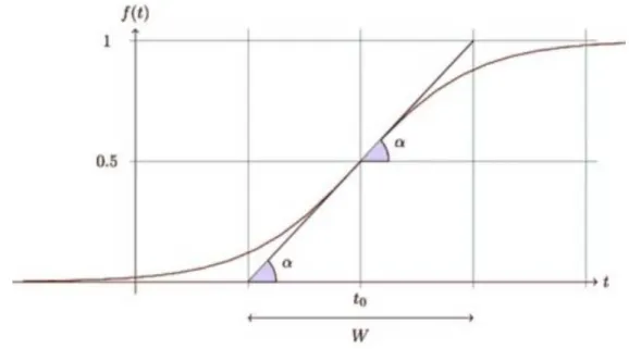
Basically, MOA stream generators add artificial concept drifts into the examples inside a stream. We should consider data streams generated from a pure distribution, thus Concept drift models as a weighted combination of two pure distributions in order to characterize the target concept before and after the drift. MOA for achieving a probability to define if a new instance of a stream belongs to the new concept after the drift or not, uses sigmoid function as shown in Figure 3.2

According to Figure 3.2, the sigmoid function f (t) = 1/(1 + e−s(t−t0)_{) has a}

derivative at the point t0 equal to f’(t0) = s

4. The tangent of angle is equal to this

derivative, tan α = s

4. We observe that α = 1

W, and as s =4 tan α then s = 4

W. So the

parameter s in the sigmoid gives the length of W and the angle α. In this sigmoid model we only need to specify two parameters t0 the point of change, and W the

length of change.

3.2.4 Concept Drift Generator

(40)

20 MOA Framework

Figure 3.2: A sigmoid function f (t) = 1/(1 + e−s(t−t0)₎

Abrupt change generator

Any change in the parameters of the system that occurs either instantaneously or at least very fast with respect to the sampling period of the measurements can be defined as Abrupt change. In order to recreate this instantaneously drift, this generator produces a huge amount of instances all with the same value, then a setting instance changes the value and replicates it until the end.

Gradual change generator

As the term itself indicates, the gradual change allows a gradual increase in the value of the instances. This is a scenario where one concept fades gradually while the other takes over. A real-world example, to better understand it, is that of a device that begins to malfunction. At the beginning only a small number of data points will come from the stable failure state. Finally, the failure value will take over completely.

Incremental change generator

In this case, concept drift, is characterized by an incremental modification of the current concept toward a future concept. In order to recreate this kind of situation we have generated a stream of data that represents an incremental change. We based

(41)

3.2 How it works 21

our dataset on a function f (x) = mx + ε where m is a constant value of 0,40, x is an incremental value starting from 1000 and ε is a random value between -100 and +100.

(42)

(43)

Chapter 4 Il Paese Ritrovato Dataset

In this chapter we briefly present the system of Il Paese Ritrovato, a healthcare facility located in Monza that was created for the residential care of people affected by the Alzheimers disease. In particular we talk about the data collected that are available for our project and how we calculate the indexes to asses the wellness of the patients.

4.1 Il Paese Ritrovato

Il Paese Ritrovato is organized as a small town, where people lead a healthy life, feeling at home and receiving the necessary attention at the same time. The purpose of this place is to slow down the cognitive decline and minimize disabilities in everyday life, offering the resident the opportunity to continue to live a life that is rich and appropriate to his abilities, desires and needs.

4.2 The Pervasive System

The inhabitants of Il Paese Ritrovato are always followed through non-invasive devices, both environmental (advanced domotics) and physiological (wearable sensors), to guarantee adequate support for residual autonomy and help with daily difficulties. In particular, these technological tools help clinicians and professionals to continuously monitoring the wellness of the patients. The leading technologies are a localization system, that has the role of control and collecting patients’ data, and a system that registers different indicators related to the well-being of the patients.

(44)

24 Il Paese Ritrovato Dataset

4.2.1 Localization system

The localization system in the health-care home is based on an RSSI (Signal strength indicator received) methodology useful for estimating a human position in an indoor location system. This type of technology allows us to calculate the patient’s position by attributing to the strongest signal.

4.2.2 Indexes of Well-being

Through the use of location data, it has been possible to generate indicators that can be continuously calculated and analyzed, providing useful information to monitor an individual’s state of well-being. The indicators are the following:

• Distance index: indicates the number of meters a patient takes during the day. Its value is calculated by exploiting the potential and the dynamics of the localization system. Knowing the distances between a position detector and the other a priori, it is possible to understand and calculate the movements of the individual patients simply by observing all the cells to which the patient has hooked during the day and calculating the total distance.

• Movement Index: is based on the detection of distances. Through this index we have an estimate of the quality and quantity of movements that a patient performs during the day. Each patient has a value, expressed in meters, that he should reach during the day. Based on the detection of the distance traveled to each patient, it is possible to calculate the movement index, which can take values between 0 (small movement) and 1 (sufficient movement).

• Sleep Index: the localization system registers the hours and the number of interruptions of the patients sleep by checking the signal of vicinity to the bed antennas during the night.

• Isolation Index: is based on the number of people the system locates in the same area as the monitored patient. This index can take values between 0 and 1, wherein the first case, the person examined has never been close to other people, while in the second one it has been close to other people all day. • Independence Index: assesses a patient’s level of autonomy. As for the

(45)

4.3 Issues and Artifacts 25

the person monitored is in the company of doctors, health professionals and operators. It has a value between 0 and 1.

• Relational Index: estimates the relationship between two people by quanti-fying the amount of time they spend together in one day. When the two people monitored have never been in the same area of interest then their relational value will be zero, otherwise, in the opposite case in which the two people share the same spaces for the whole day then their index will assume a value equal to 1.

For the experiment (Chapter 5 Section 5.4.3), we used distance indices for a period of observation that starts from February 1st and ends on the 25th of August of this year.

4.3 Issues and Artifacts

During the data collection’s phase, to carry out our experiment, we met, managed and solved various types of problems related to data consistency and the missing values. As shown in Figure 4.1 we can notice different kinds of data problems. One of the first problems that can be noticed is the lack of values in some periods of observation (Figure 4.1(a)), more or less lasting over time. This particular type of problem can be caused by various factors such as the loss of the antenna connection, the lack of maintenance relative to the battery of patient bracelets when the latter discharges or fails due to external problems such as the presence of water in the bracelet. In figure 4.1(b) there is another type of problem we had to deal with, that refers to the peaks of anomalous and inconsistent values with the rest of the dataset. The main causes of this problem are due to the loss of the closest antenna connection. When it happens, the bracelet worn by the person tries to hook onto the first available antenna with the strongest signal. If the patient is found in the presence of more antennas, the signal will be bounced between the different receivers and in our dataset it will seem that the patient in observation has walked for many meters even if it is not true. The last type of problem observed, as shown in Figure 4.1(c), consists in the fact that not all the monitored patients stayed in the ”Il Paese Ritrovato” health care home during the whole observation period of the experiment. We have noticed that some patients had an initial or final period of observation with all the values equal to 0. Going

(46)

26 Il Paese Ritrovato Dataset

deeper, we found that these patients arrived after the start date of the observations or left before the end of the experiment.

(a) Missing Value (b) Inconsistent Value (c) Period not evaluated

Figure 4.1: Different types of issues related to the dataset

4.4 Proposed Solution

We have decided to deal with the issue in Section 4.3 in the following way:

• To overcome the problem of the presence of null or missing values we decided to replace them with the average of the remaining values relative to the period of the individual patient.

• For the problem of inconsistent values we decided to calculate the standard deviation on the period of interest. When a value in this range exceeded three times the value of the standard deviation, the latter was replaced by the average value previously calculated.

• For patients who were not present for the entire duration of the experiment we decided to observe them only during their presence going to eliminate null values that could alter the results of the experiment.

4.5 Simulated Dataset

Based on the experience of Il Paese Ritrovato the Department of Electronics Informa-tion and Bioengineering of the Politecnico di Milano located in Como has created a software that allows the simulation of life inside a health care house. The engineers of the Politecnico have recreated the plan of the Il Paese Ritrovato, also positioning the various position detectors in the relative places. Later, this simulated house was pop-ulated by users who, as real patients, have constraints and needs and therefore move

(47)

4.5 Simulated Dataset 27

within the virtual home to meet their needs. Through this software, it was possible to overcome the problems listed in Section 4.3, and it was also possible to simulate behavioral drifts within some patients in the index that monitors the distance trav-eled. For the experiment, the system generated eight users and their movements were simulated for 3 years from 1 January 2016 to 31 July 2019.

(48)

(49)

Chapter 5 Experiments and Discussion

This chapter starts with a description about the main goal of performing experiments with MOA, then the following section explains the experiments set up regarding the main goal. Finally, the output of experiments is reported and in the last part, there is a discussion and comparison about the results of experiments.

5.1 Description

The objective is to detect the behavioral drifts in a Health-Care Facility dataset. In order to reach it, all the concept drift detection methods implemented in MOA have been used with different datasets with different kinds of drifts. To detect the best methods the accuracy, the average prediction error, the number of false positives, the number of false negative and the average delay detection in term of instances have been analyzed.

5.2 Experiments Set Up

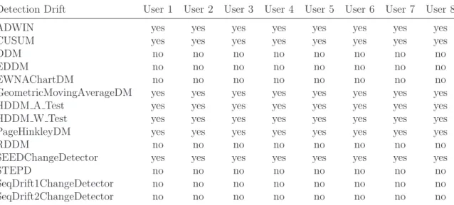
To understand if the concept drift detectors in MOA can detect the behavioral changes, three types of experiments have been done. In the first experiment, as shown in table 5.1, we have tested all the detection methods that are present in MOA on all the different types of Real Drift. During this part, we have used a function implemented in MOA that gives us the possibility to generate a dataset in which there are different kinds of real drifts as shown in figure 5.1. Once understood which kind of drift is able to detect each algorithm, we have analyzed the results.

(50)

30 Experiments and Discussion

(a) Single Abrupt (b) Cyclic Abrupt (c) Gradual

(d) Single Incremental (e) Cyclic Incremental

Figure 5.1: Different type of drifts generated by MOA framework

After that we have seen if the results are equal if we use simulated datasets regarding home daily activates. In the end of our experiment, we tested these methods on a real dataset coming from the health care house Il Paese ritrovato in Monza. For the first part of the experiment we used Naive Bayes as base learner in all tested drift detection methods, because of its speed, simplicity, freely available implementations, and widespread use in experiments in the data stream research area [26]. Another important setting is what concerns the SingleClassifierDrift that is a classifier imple-mented in MOA which tests each incoming instance using a base learner, in our case Naive Bayes, which returns a boolean value indicating if it correctly classified the instance or not. This value is passed to the parameterized drift detector analysed, which will flag the example for no drift, warning level, or drift level. If no drift is identified, the base learner is trained on the instance just arrived. If the warning level is reached, a new learner is built and both are trained. If the drift level is reached, the learner built on instances obtained in the warning level is used as the new base learner. Important to know is that ADWIN method does not have a warning level to set up beacuse ADWIN is parameter- and assumption-free in the sense that it automatically detects and adapts to the current rate of change [5].

5.3 Experiment Evaluation

The most important properties in data drift detection are the following:

(51)

5.3 Experiment Evaluation 31

occurred, but it has not occurred yet in the data stream.

• False Negative (FN): happens when a change has in fact occurred, but the algorithm has failed to detect it yes. Also known as a miss.

• Accuracy: Its value is a percentage of the correct prediction over a given dataset by a model. It is given by the following formula:

Accuracy = T P + T N

T P + T N + F P + F N

where TP stands for TRUE POSITIVE and TN for TRUE NEGATIVE. They are the number of times in which the algorithm correctly predicted.

• Prediction Error: is the difference between the actual value (AV) and the predicted value(PV) for that instance. If the base learner correctly classifies the actual instance, the error-rate decreases. Instead, if the error-rate increases, it is an indication of Concept drift. The tables 5.2, 5.3, 5.4, 5.5, 5.6 show the average prediction error that refers to the mean of the absolute values of each prediction error on all instances (n) of the test dataset as in the following formula: n P i₌₁ |AVi− P Vi| n

• Delay Detection Avg in terms of instances it is the average number of instances between the moment in which the real drift occurs and the moment in which the algorithm catches the drift.

In general, the best algorithm will have a minimal number of false alarms and max-imal number of early detections, whereas poor algorithms give large number of false alarms, missing or severely delayed true detections. In order to evaluate a model in MOA framework, after an experiment completes, MOA provides a .txt format file as an output which contains several information regarding to learning evaluation in-stances, evaluation time (CPU/seconds), model cost (RAM-Hours), learned inin-stances, detected changes, detected warmings, prediction error (average), true changes, delay detection, true changes detected, inputs values, model training instances, model se-rialized size (byte) that can be used for evaluation tasks. Among all properties, our

(52)

focus is on prediction error, change detected, and also on true changes and true changes detected that have been useful to identify false positive and false negative.

Detection Drift ABRUPT SINGLE ABRUPT CYCLIC GRADUAL INCREMENTAL INCREMENTAL CYCLIC NO DRIFT

ADWIN YES YES YES YES YES NO

CUSUM YES YES YES YES YES NO

DDM YES YES YES NO NO NO

EDDM NO YES YES NO NO NO

EWNAChartDM YES YES YES NO NO NO

GeometricMovingAverageDM NO NO NO YES YES NO

HDDM A Test YES YES YES YES YES NO

HDDM W Test YES YES YES YES YES NO

PageHinkleyDM YES YES YES YES YES NO

RDDM YES YES YES NO NO NO

SEEDChangeDetector YES YES YES YES YES NO

STEPD YES YES YES NO NO NO

SeqDrift1ChangeDetector YES YES NO NO NO NO

SeqDrift2ChangeDetector YES YES YES NO NO NO

Table 5.1: The table shows which type of drift each method is able of detect in the first part of our experiment

5.4 Results

All experiments are carried out using MOA (Massive Online Analysis). We have considered three variations of concept drifts: Abrupt drift (single and cyclic), Gradual drift and Incremental drift (single and cyclic) on all the drift detection algorithms listed above. All the methods are analyzed with the properties written in the previous section.

5.4.1 Experiments on MOA generetor Dataset

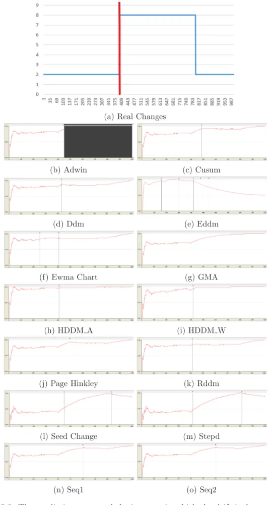
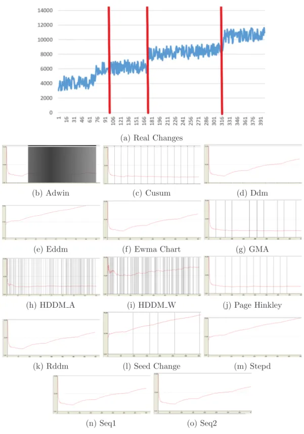
As highlighted in Subsection 5.3, one of the most important measure to analyze a drift is the prediction error. In order to measure its performance we need to show and compare the trend over time for all the algorithms. In the following figures starting from Figure 5.2 to Figure 5.6, is possible to see with the red vertical line the real changes that occur in the trends, with the red horizontal line the trends of the prediction error of the all algorithms presented and with the vertical black line the instance in which the drift is detected. Then, tables for each kind of drift with their respective values are reported.

(53)

5.4 Results 33

(a) Real Changes

(b) Adwin (c) Cusum

(d) Ddm (e) Eddm

(f) Ewma Chart (g) GMA

(h) HDDM A (i) HDDM W

(j) Page Hinkley (k) Rddm

(l) Seed Change (m) Stepd

(n) Seq1 (o) Seq2

Figure 5.2: The prediction error and the instance in which the drift is detected in an Abrupt drift

(54)

(a) Real Changes

(b) Adwin (c) Cusum

(d) Ddm (e) Eddm

(n) Seq1 (o) Seq2

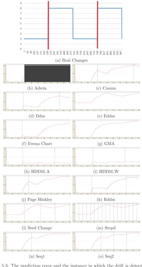
Figure 5.3: The prediction error and the instance in which the drift is detected in a cyclic Abrupt drift

(55)

5.4 Results 35

(a) Real Changes

(b) Adwin (c) Cusum

(d) Ddm (e) Eddm

(n) Seq1 (o) Seq2

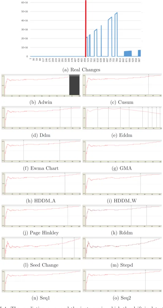
Figure 5.4: The prediction error and the instance in which the drift is detected in a Gradual drift

(56)

(a) Real Changes

(b) Adwin (c) Cusum (d) Ddm

(e) Eddm (f) Ewma Chart (g) GMA

(h) HDDM A (i) HDDM W (j) Page Hinkley

(k) Rddm (l) Seed Change (m) Stepd

(n) Seq1 (o) Seq2

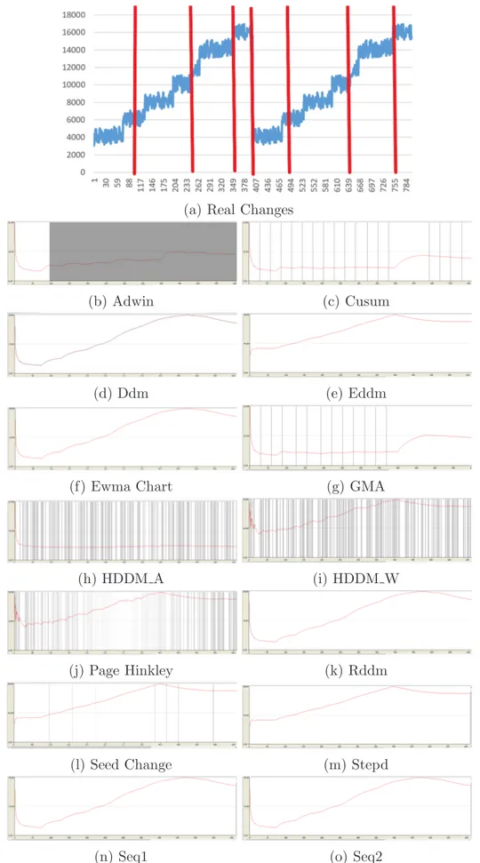
Figure 5.5: The prediction error and the instance in which the drift is detected in an Incremental drift

(57)

5.4 Results 37

(a) Real Changes

(b) Adwin (c) Cusum

(d) Ddm (e) Eddm

(n) Seq1 (o) Seq2

Figure 5.6: The prediction error and the instance in which the drift is detected in a cyclic Incremental drift

(58)

38 Experiments and Discussion CYCLIC ABRUPT ACCURACY PREDICTION ERROR FALSE POSITIVE FALSE NEGATIVE DELAY DETECTION AVG IN INSTANCE

ADWIN 91,6 1,870957513 708 0 20 CUSUM 92,4 1,18330909 0 0 131 DDM 96,3 1,136879686 0 0 54 EDDM 93,8 1,977433331 0 2 -EWNAChartDM 96,3 1,084511709 0 1 3 GeometricMovingAverageDM 92,4 1,379083686 0 2 -HDDM A Test 96,1 1,441276203 0 0 12 HDDM W Test 95,2 1,343241626 0 0 30 PageHinkleyDM 92,4 1,191895544 0 1 52 RDDM 96,3 1,393502248 0 0 32 SEEDChangeDetector 94,8 1,977433331 2 0 29 STEPD 95,8 1,977433331 14 0 41 SeqDrift1ChangeDetector 92,4 1,392201718 0 1 75 SeqDrift2ChangeDetector 92,4 1,371532301 1 0 101

Table 5.3: Evaluation of concept drift detector on a cyclic abrupt generated by MOA

GRADUAL ACCURACY PREDICTION ERROR FALSE POSITIVE FALSE NEGATIVE DELAY DETECTION AVG IN INSTANCE

ADWIN 79,1 1,949961108 135 0 365 CUSUM 75,7 1,910575481 0 0 340 DDM 80 1,92061238 1 0 235 EDDM 80,2 1,674491942 8 0 76 EWNAChartDM 82,2 0,019531705 1 0 231 GeometricMovingAverageDM 41,4 1,972260302 0 1 -HDDM A Test 82,5 0,19637868 0 0 99 HDDM W Test 82,2 0,196235537 0 0 242 PageHinkleyDM 64 0,191514408 0 0 346 RDDM 81,2 1,924514432 1 0 119 SEEDChangeDetector 80,5 1,648296593 1 0 269 STEPD 81,8 1,648296593 0 0 243 SeqDrift1ChangeDetector 60,6 1,972260302 0 1 -SeqDrift2ChangeDetector 60,6 0,193226746 0 0 301

Table 5.4: Evaluation of concept drift detector on a gradual drift generated by MOA

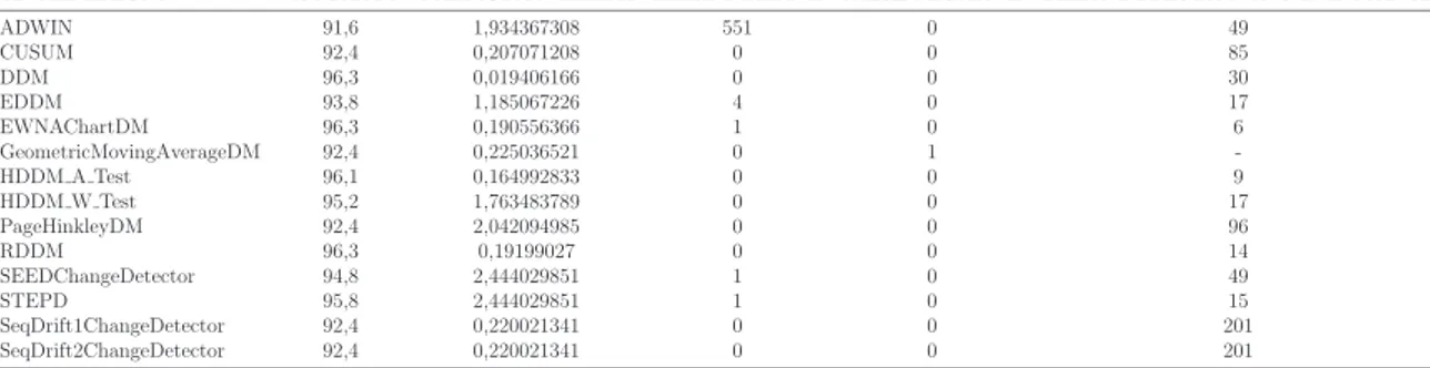
SINGLE ABRUPT ACCURACY PREDICTION ERROR FALSE POSITIVE FALSE NEGATIVE DELAY DETECTION AVG IN INSTANCE

ADWIN 91,6 1,934367308 551 0 49 CUSUM 92,4 0,207071208 0 0 85 DDM 96,3 0,019406166 0 0 30 EDDM 93,8 1,185067226 4 0 17 EWNAChartDM 96,3 0,190556366 1 0 6 GeometricMovingAverageDM 92,4 0,225036521 0 1 -HDDM A Test 96,1 0,164992833 0 0 9 HDDM W Test 95,2 1,763483789 0 0 17 PageHinkleyDM 92,4 2,042094985 0 0 96 RDDM 96,3 0,19199027 0 0 14 SEEDChangeDetector 94,8 2,444029851 1 0 49 STEPD 95,8 2,444029851 1 0 15 SeqDrift1ChangeDetector 92,4 0,220021341 0 0 201 SeqDrift2ChangeDetector 92,4 0,220021341 0 0 201

(59)

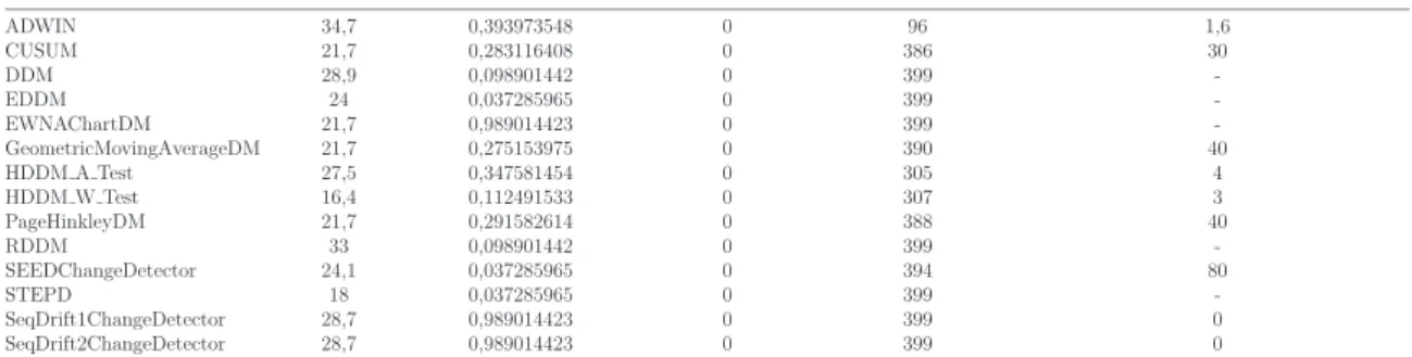
5.4 Results 39 INCREMENTAL ACCURACY PREDICTION ERROR FALSE POSITIVE FALSE NEGATIVE DELAY DETECTION AVG IN INSTANCE

ADWIN 34,7 0,393973548 0 96 1,6 CUSUM 21,7 0,283116408 0 386 30 DDM 28,9 0,098901442 0 399 -EDDM 24 0,037285965 0 399 -EWNAChartDM 21,7 0,989014423 0 399 -GeometricMovingAverageDM 21,7 0,275153975 0 390 40 HDDM A Test 27,5 0,347581454 0 305 4 HDDM W Test 16,4 0,112491533 0 307 3 PageHinkleyDM 21,7 0,291582614 0 388 40 RDDM 33 0,098901442 0 399 -SEEDChangeDetector 24,1 0,037285965 0 394 80 STEPD 18 0,037285965 0 399 -SeqDrift1ChangeDetector 28,7 0,989014423 0 399 0 SeqDrift2ChangeDetector 28,7 0,989014423 0 399 0

Table 5.5: Evaluation of concept drift detector on a incremental drift generated by a function

CYCLIC INCREMENTAL ACCURACY PREDICTION ERROR FALSE POSITIVE FALSE NEGATIVE DELAY DETECTION AVG IN INSTANCE

ADWIN 34,7 0,656355278 0 96 1,3 CUSUM 21,7 0,529118145 0 774 33 DDM 28,9 0,177053197 0 798 -EDDM 24 0,489013784 0 798 -EWNAChartDM 21,7 0,177053197 0 798 -GeometricMovingAverageDM 21,7 0,065470756 0 780 38 HDDM A Test 27,5 0,36164787 0 596 4 HDDM W Test 16,4 1,621490387 0 581 3,6 PageHinkleyDM 21,7 0,086348959 0 784 57 RDDM 33 0,177053197 0 798 -SEEDChangeDetector 24,1 0,489013784 0 785 61 STEPD 18 0,489013784 0 798 -SeqDrift1ChangeDetector 28,7 0,177053197 0 798 -SeqDrift2ChangeDetector 28,7 0,177053197 0 798

-Table 5.6: Evaluation of concept drift detector on a cyclic incremental drift generated by a function

Change detection is a significant element of systems that need to adapt to changes in their input data. DDM and RDDM work well for detecting abrupt changes both with single and cyclic and reasonably fast changes founding drifts in the right moment that occur, but they have difficulties in detecting slow, gradual changes and incremen-tal ones too. For abrupt drift, the CUSUM method is the one that is able to detect the right drift but with the highest value in terms of delay followed by Seq1 and seq2. In addicti. The last thing that we can see in abrupt drift is that PageHinkle finds the right number of drifts with a soft delay but has a low accuracy compared with the others. For Gradual drift, considering the results, HDDMA-test and HDDMW-test

have high accuracy and they are able to detect the right number of changes with a relative delay. Another method that has a good performance in Gradual drift is the EDDM. It found the right drift on time (delay is approximately 0) and with a very low prediction error on average. We can say that, considering a quality/cost trade off, for gradual drift the most performing is the EDDM algorithm. ADWIN, instead,

(60)

seems to be the algorithm with the best results for incremental drift where all the other kinds of methods fail dramatically.

5.4.2 Experiments on Simulated Dataset

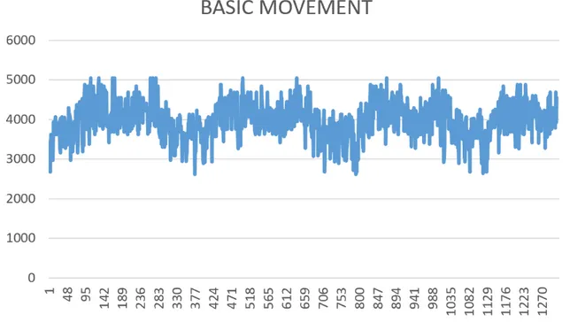
During this phase, we have analysed a dataset coming from software that simulated the behavior of patients during their permanence in a health care facility. We will focus on evaluating the number of drift that each method is able to detect. Moreover, we will try to understand which of them doesn’t recognise the periodicity and the glitch that could stay in the data. This dataset contains record starting from the 1st January 2016 to the 31st July 2019 of 8 patients. Each trend is built based on a sinusoidal pattern, that simulates the movement of a person, without drift, during the different season that occurs during the years. More in detail, it has been created from the relation between the weather ( temperature, weather conditions, humidity) in Milan in the last 3 years and the distance made by a patient of the Healt-care Facility Il Paese Ritrovato as explained in Chapter 4.

Figure 5.7: Sinusoidal trend, that simulates the movement of a person, without drift, during the years

Comparison of concept drift detectors in a health-care facility dataset to detect behavioral drifts