A class of spatial econometric methods in the empirical analysis of clusters of firms in the space

! " # $ % & ' ( ) % * ! +,- "' . ! /0!/

A class of spatial econometric methods in the empirical

analysis of clusters of firms in the space

1

Giuseppe Arbia

2

, Giuseppe Espa

3

and Danny Quah

4

Abstract: In this paper we aim at identifying stylized facts in order to suggest adequate models of spatial co–agglomeration of industries. We describe a class of spatial statistical methods to be used in the empirical analysis of spatial clusters. Compared to previous contributions using point pattern methods, the main innovation of the present paper is to consider clustering for bivariate (rather than univariate) distributions, which allows uncovering co–agglomeration and repulsion phenomena between the different industrial sectors. Furthermore we present the results of an empirical application of such methods to a set of European Patent Office (EPO) data and we produce a series of empirical evidences referred to the the pair–wise intra–sectoral spatial distribution of patents in Italy in the nineties. In this analysis we are able to identify some distinctive joint patterns of location between patents of different sectors and to propose some possible economic interpretations.

JEL classification: C21; D92; L60; O18; R12

Keywords: Agglomeration; Bivariate K–functions; co–agglomeration; Non parametric concentration measures; Spatial clusters; Spatial econometrics.

1. Introduction

The dominating feature of economic activities is certainly that of clustering both in space and time. However, even if the application of statistical techniques for modelling clustering in time (business cycles) has been a central concern of applied economists for decades, it is only relatively recently that the research has concentrated on the development of appropriate methods to detect spatial clustering of economic activities both on a discrete space and on a continuous space.

The possibility of modelling the spatial dimension of economic activities is of paramount interest for a number of reasons. First of all the study of spatial concentration of economic activities can shed light on economic theoretic hypotheses concerning the nature of increasing returns and the determinants of agglomeration. These hypotheses are of paramount importance in international trade and in economic growth theories. A second important reason is constituted by the fact that the effects of policy measures to foster economic growth and development are strongly dependent on geographical clustering. Finally spatial clustering, as a synonym of regional inequality, is a central political issue as a proxy of individual inequality and as the basis for cross–country inequality.

After the recent reinterpretation of Marshall's (Marshall, 1890) insights on 19th–century industrial clustering in space due mainly to Krugman (1991) and Fujita et al. (1999), the empirical analysis on this subject has developed along two distinct lines of research. Along the first of these two lines in the literature we record attempts to examine directly the underlying economic mechanism, using the spatial dimension primarily as a source of data. Under this respect panel data or pure spatial regressions are used, employing observable covariates related to space. Such

1

A previous version of this paper was presented at the Workshop on Spatial Econometrics and Statistics, held in Rome 25th to 27th of may 2006. We wish to thank the participants for the useful comments received.

2

Corresponding author: Department of the Business, Statistical, Technological and Environmental Sciences, University “G. d’Annunzio” of Chieti–Pescara, Viale Pindaro, 42, 65127 Pescara, Italy, arbia@unich.it.

3

Department of Economics, University of Trento, via Inama, 5, 38100, Trento, Italy, giuseppe.espa@economia.unitn.it. 4

Economics Department, London School of Economics, Houghton Street, London WC2A 2AE, UK,

regressions end up constructing a hypothetical representative unit (a “site”) and concentrate on the impact of differing covariate values on the performance of that representative unit (see e. g. Ciccone and Hall, 1996; Jaffee, et al., 1993; Rauch, 1993; Henderson, 2003).

Here we follow the second line of research which attempts to characterize the entire spatial distribution of economic activities relative to a set of hypotheses (e. g. a certain regularity patterns of industrial concentration). In this second instance interest does not rests on the characteristics of a

representative unit, but rather on the joint behaviour of the different units distributed across space.

Along these lines Duranton and Overman (2005) refer to three generations of measures of spatial concentration. A first generation considered Gini–type measures where space played no rule (e. g. Kurgman, 1991). A second generation (perhaps initiated by Ellison and Gleaser, 1997) introduced measures that take into account space and tend to control for the underlying industrial concentration (Maurel and Sedillot, 1999; Devereuex et al., 2004). Such measures are based on data observed on a grid of administrative areas thus neglecting the problem of the arbitrariness of the geographical partition used: this problem is known in the statistical literature as the Modifiable Unit Problem (Yule and Kendall, 1950) and assumes here the specific facet of the Modifiable Areal Unit Problems (or MAUP) discussed at length in Arbia (1989). Arbia (2001) and Duranton and Overman (2005) provide an exhaustive account of the advantages of a third generation of measures that look at maps of points on a continuous, rather than on a discrete, space: following this approach we can easily compare the results across different scales.

In the present paper we look at the distribution of industries as a map of points in the space and we characterize their geographical distribution through the Lotwick–Silverman (Lotwick and Silverman, 1982) extension of the spatial statistical non–parametric tool known as the K–function (Ripley, 1977). The use of the K functions in economic analysis was first introduced in the literature by Arbia and Espa (1996) and then exploited by Marcon and Puesch (2003a; 2003b), by Quah and Simpson (2003) and by Duranton and Overman (2005) amongst the others. Ioannidis and Overman (2004) look also at the properties of points on a continuous space, but using a different approach. Compared to previous contributions the major innovation of the present paper is to consider clustering for bivariate (rather than univariate) distributions, which allows uncovering agglomeration and repulsion phenomena between different sectors. The literature often refers to this subject as to co–agglomeration or co–localization (Devereux, et al., 2004; Duranton and Overman, 2005). The functionals we propose to characterize a joint pattern of points satisfies the five conditions suggested by Duranton and Overman (2005) for a concentration measure5. In particular we introduce the use of the K function to control for the underlying industrial concentration.

The theoretical ground on which such a modelling framework is based is well described in Quah and Simpson (2003) where the authors stressed the importance of being able to specify a model determining a spatial law of motion and its evolution through time. Quah–Simpson model assumes that each individual economic agent aims at maximizing his own profit by locating his activity where the average spatial return is higher with a gradual time–adjustment based on a cost function. Equilibrium is then achieved by optimizing the choices of each individual economic agent. The result is a (space–time) partial differential equation that expresses the economic activity in each point in time and space as a density. A good way of approaching the empirical analysis of clusters in space is then represented by a modelling framework that is able to describe how such densities change in space conditionally upon the observed pattern of points.

A field were what Quah and Simpson (2003) define as a spatial law of motion is particularly theoretically grounded is the analysis of the spatial diffusion of innovation and of technological spillovers. For this reason the empirical part of this paper is devoted to the analysis of the joint location of innovations.

5

The five requirements suggested by Duranton and Overman (2005) for a concentration measure are the following: any measure (i) should be comparable across industries; (ii) should control for the overall agglomeration of manufacturing; (iii) should control for industrial concentration; (iv) should be unbiased with respect to scale and aggregation; and, finally (v) should also give an indication of the significance of the results.

The studies on knowledge spillovers have received increasing importance in the literature on economic growth. In fact some theories explicitly link the presence of innovations to the growth of cities (Jacobs 1969, 1984; Bairoch 1988) seen as the places where the big concentration of individuals, firms and workers create positive externalities which, in turn, foster economic growth. Even if economic theory has produced important advances in this direction (Arrow 1962; Romer 1986; Lucas 1988; Porter 1990) empirical evidences are still largely lacking. In fact a large part of the empirical literature concentrated on measuring the impact of technological spillovers on the innovation performances of regions. In many instances the number of patents and the patents citations have been used as a proxy of the flow of knowledge and of the related innovative output (Jaffe and Trajtenbergerg, 1996; 2002; Jaffe et al., 2000). One possible approach is based on the notion of knowledge production function introduced by Griliches (1979) which links regional innovative output with measures of regional innovative inputs like R&D expenses (see e. g. Jaffe 1989; Audretsch e Feldman 1996; Acs et al. 1994). These studies provide significant evidences of the impact of localized R&D inputs on the innovation performances of regions. There are comparatively less empirical evidences on the effects of localized knowledge spillovers (Glaeser et

al. 1992; Henderson and Kunkoro 1995; Henderson 2003) and no definite answer is yet available to

the question whether knowledge flows are favoured by regional specialization within firms or, vice versa by industrial diversification.

In this paper we wish to show the importance of the distance–based measures of spatial concentration in tackling this important emerging research area and to provide new statistical tools to study the complex interaction between spatial concentration, regional growth and knowledge spillovers. The layout of the paper is the following. In Sections 2 and 3 we will thoroughly review the statistical reference framework by presenting a set of tools to identify clusters of industries in the space. Specifically in Section 2 we will concentrate on the bivariate version of Ripley’s (Ripley, 1977) K function whereas in Section 3 we will discuss the system of hypotheses at the basis of the identification of clusters and by distinguishing two possible null hypotheses to be contrasted with the hypothesis of spatial clustering of industries. Section 4 is devoted to the analysis of the results of an empirical application of the bivariate K function in the study of the inter–sectoral location of innovation in Italy based on a dataset of the European Patent Office (EPO) which records all patent applications in Europe. Finally Section 5 contains some conclusions and directions for further developments in the field.

2. The statistical theoretical framework: bivariate K functions

Univariate K–functions (proposed by Ripley, 1976; 1977) have been already used in economic geography to characterize the geographical concentration of industries (see e. g. Arbia and Espa, 1996; Marcon and Puech, 2003a; Quah and Simpson, 2003). In this paper we will consider a bivariate extension of such a method to describe spatial clusters of pairs of firms. Although the approach could be straightforwardly generalized to an arbitrary number of, say, g (g>2) industries, in this paper we will deliberately restrict ourselves to the bivariate case for the sake of illustrating the methodology. The method is based on a bivariate functional of distance t (that we will refer to as

( )

t

Kij ) which characterizes the joint spatial pattern of points or, more precisely, the spatial

relationships between two typologies of points located in the same study area: for instance firms belonging to two different industrial sectors, say Type i and Type j. The bivariate K function is defined as follows:

( )

t 1E

{

#of pointsofTypeifallingat adistance tfroman arbitray Type jpoint

}

K_ij =_λ−_j ≤

with E

{}

⋅ indicating the expectation operator and the parameter λ_j representing the intensity of Type j point process, that is the number of Type j points per unitary area. Obviously, in the presence of a multivariate point process we have g typologies of events and, consequently, g bivariate K 2 functions that is : K₁₁

( )

t , K₁₂

( )

t , …, K_1g

( )

t , K₂₁

( )

t , K₂₂

( )

t , …, K_2g

( )

t , …, K_gg

( )

t . In the remainder we will clearly distinguish between univariate and bivariate K functions by calling auto–

functions K those for which i= and cross–functions K those for which j i≠ . Conversely, when j j

i= , K_ii =K_i is the more traditional univariate auto–function K used in the economic analysis by e. g. Quah and Simpson (2003), Marcon and Puesh (2003a) and Duranton and Overman (2005).

In Equation [1], the term λ_jK_ij

( )

t represents the expected number of Type j points falling within a circle of radium t centred on an arbitrary Type i point. Symmetrically we interpret the bivariate function K_ji

( )

t in such a way that λ_iK_ji

( )

t represents the expected number of Type i points falling within a circle of radium t centred on an arbitrary Type j point. Similarly to the case of univariate K function, also the bivariate K function is built under the assumption of isotropy (see Arbia, 2006) that is the case when no directional bias occurs in the neighbourhood of each point.

In a bivariate point map constituted by, say, n_i points of Type i and n_j points of Type j within an area A, we can define a class of estimators of the cross–functions K by close analogy to those suggested in the univariate case (Ripley, 1977; Diggle, 1983).

To start with, let us consider the indicator function:

I_lk

( )

t = 1 if dlk ≤ t

0 if d_lk> t ⎧

⎨ ⎩

where d_lk represents the distance between the l–th Type i point and the k–th Type j point. If no border effects are present, then the non–parametric estimator of the cross–function K_ij

( )

t can be expressed as:

( )

(

)

_∑∑

( )

= = − = 1 2 1 1 1 ˆ ˆ ˆ n l n k lk j i ij t A I t K λλ

where A is the total surface of the area,

A n_i i = λˆ _and A n_j j = λˆ _.

Analogously, by inverting the role between Type i and Type j points, the corresponding non– parametric estimator for the cross–functionK_ji

( )

t is given by:

( )

(

)

_∑∑

( ) ( )

= = − − = 2 1 1 1 1 1 ˆ ˆ ˆ n l n k lk lk j i ji t A t J t K λλ ν

with ν_lk

( )

t and J_lk

( )

t analogous to the I_lk

( )

t functions in the previous expression.

If the generating random field is stationary and isotropic (Arbia, 2006), then K_ij

( )

t should be equal to K_ji

( )

t . However, due to possible border effects6 and to the asymmetry of the related corrections, ˆ K _ij

( )

t and ˆ K _ji

( )

t will be not exactly equal although strongly correlated. A more

6

On “border effects” and corrections for them see e. g. Ripley (1981). Explicit expressions of the correction factors in the case of irregular study areas are derived in Goreaud and Pélissier (1999).

efficient (although not absolutely efficient) estimator is thus the one proposed by Lotwick and Silverman (1982) given by:

( )

( )

( )

j i ji i ij j ij t K t K t K λ λ λ λ ˆ ˆ ˆ ˆ ˆ ˆ * + + = . [2]

Likewise Ripley’s univariate K function, also in the case of the multivariate functions we can introduce the L transformation proposed by Besag (1977) which is characterized by a more stable variance. In the bivariate case the Lˆ_ij

( )

t functions assume the expressions:

ˆ

L _ij

( )

t = ˆ K _ij

( )

t π [3]

and ˆ

L _ji

( )

t = ˆ K _ji

( )

t π [4]

where the functions are linearized dividing by π and the square root stabilizes the variance. Similarly to Equation [2] we can consider the Lotwick–Silverman transformation

L*_ij t

( )

=λ ˆ jL ˆ ij

( )

t + ˆ λ iL ˆ ji

( )

t ˆ λ _i+ ˆ λ _j = K * ji

( )

t π [5]

which produces more efficient estimators of the L function.

3. The basic hypotheses of the model: spatial independence or random labelling?

In this section we wish to introduce various alternatives offered in the spatial statistical literature to specify the null hypothesis of absence of regularities in the location of pairs of points in space. These will represents our counterfactuals in the subsequent empirical analysis reported in Section 4.2. In order to correctly interpret the estimates provided by K_ij*

( )

t and L*_ij

( )

t to test the null hypothesis of absence of spatial interaction, traditionally the empirical estimates are compared with simulated envelops. The reference framework for such tests is provided by Barnard (1963) and adapted by Ripley (1979) to the case of univariate spatial clusters. In the case of bivariate patterns the specification of the null hypothesis is more complicated. In fact we can have two possible definitions depending on the nature of the case examined: a null of independence and a null of

random labelling (Diggle, 1983; Dixon, 2002). The choice between the two alternatives can

strongly affect the final results and can lead to wrong conclusions. However this distinction is often ignored in the literature where the univariate procedures are sometimes uncritically applied (among the few exceptions see Diggle, 1983 and, more recently Dixon, 2002 and Goreaud & Pélissier, 2003). The two cases will now be discussed in some details.

3.1 The null hypothesis of independence

According to a first specification of the null hypothesis the two typologies of points on the map can be conceived as two populations and the resulting spatial pattern can be interpreted a priori as the outcome of two distinct point random fields. In this situation the absence of interaction between

the two components corresponds to the lack of interaction between the two generating fields. In other words, the location of points generated by the field related to Typology i is independent of the location of points generated by the field related to Typology j (Lotwick and Silverman, 1982). Under this hypothesis, therefore, K_ij

( )

t =πt2. We will refer to this first null hypothesis as to the “hypothesis of independence” and we will indicate it with the symbol H1₀.

If within the circle of radius t centred on an arbitrary Type i point we record the presence of more Type j points than we expect under H1₀, then K_ij

( )

t >πt2 which represents the surface of a circle of radius t. Such a result indicates a positive dependence between the two components and, hence, the presence of agglomeration between the two generating fields. In contrast, if within the circle of radius t centred on an arbitrary Type i point we record the presence of less Type j points than expected under H1₀, then K_ij

( )

t <πt2, thus indicating repulsion (or inhibition) rather than agglomeration. The confidence band to run formal hypothesis testing procedures at the various distances can be built through Monte Carlo simulation (Besag and Diggle, 1977. See also Ripley, 1977; Goreaud & Pélissier, 2003 for details).

3.2 The null hypothesis of random labelling

According to a second specification of the null hypothesis each of the two components depends on some factor that “a posteriori” produces a differentiation between the two typologies of points. In the case of economic data, such factors can be identified in a set of explanatory variables encouraging location of industries at a certain point in space and producing a different pattern in the two typologies of points. For instance they might refer to a differentiated system of taxes and incentives encouraging location of Type i point while discouraging location of Type j points. We will refer to this second hypothesis as to the “random labelling” and we will indicate it with the

symbol H₀2. The general reference framework in this second instance is that of the so–called

marked point processes (see, e. g., Diggle, 1983) that is point processes where not only the location

of each object is reported, but also an extra characteristics that differentiates between them (e. g. small and large firms, presence or absence of an innovation etc.)

Let the spatial structure of the indistinct generating process for the two typologies of points be synthesized by the univariate K auto–function (Ripley, 1977):

( )

t E

{

#points within acircleof radious taroundeach point in amap

}

K = λ where A n =

λ represents the density and n=n₁+n₂. Under H₀2, the ratio p_j = nj

n represents the probability to belong to typology j. Then we have

that p_jλK

( )

t =λ_jK

( )

t =λ_jK_ij

( )

t so that K_ij

( )

t = K

( )

t . If within the circle of radius t centred on an arbitrary Type i point there are more Type j points than expected under H₀2, then K_ij

( )

t >K

( )

t . This result indicates that at distance t the two components tend to be positively dependent, thus revealing the presence of agglomeration. On the contrary, if within the circle of radius t centred on an arbitrary Type i point there less Type j points than expected under H₀2, then K_ij

( )

t <K

( )

t which indicates the presence of a negative dependence between the two components or inhibition. Again the confidence bands can be generated via Monte Carlo simulation.

When H₀2 holds true, we have that all the bivariate K functions (both the two auto–functions and the two cross–functions) are equal to the univariate K function of the map where there is no

distinction between the two components so that K_ij

( )

t =K_ji

( )

t =K_ii

( )

t =K_jj

( )

t =K

( )

t . Operationally the departures from the null of random labelling could be evaluated by computing the pairwise differences between the various K functionals and by comparing them with the simulated confidence bands (see Diggle and Chetwynd, 1991; Gatrell et al., 1996; Kulldorff, 1998; Dixon, 2002; Haining, 2003).

It is important to observe that the two alternatives for the null hypothesis considered in this section describe in statistical terms the usual distinction made in quantitative geography between two otherwise undistinguishable effects of spatial interaction between agents and spatial reaction of them to common factors (Cliff and Ord, 1981). Both effects give rise to observed regularities in space. They also mirror from a certain viewangle the distinction made by some authors in the economic literature between joint–localization and co–localization (see e. .g. Duranton and Overman, 2005).

4. Characterizing the spatial distribution of innovations in Italy 1995–1999

4.1 Descriptive analysis

The empirical analysis focuses on the use of the EPO dataset containing all patent applications made at European Patent Office (established by Monaco’s Convention) starting from 1978. In particular we use the version elaborated at CESPRI, Bocconi University, Milan. The dataset provides us with information about petitioners, inventors, request date, International Patent Classification code (distinguishing the various industrial sectors), and citations among patents. The use of the inventors’ residence allows us to localize exactly each patent (Arbia et al., 2006). In our database we omitted Sicily, Sardinia and the other Italian islands because of the lack of spatial continuity with the main land which could produce serious biases in our procedures based on Euclidean distances. The resulting dataset consists of 44,078 inventors, but only 25,312 patents due to the presence of multi–inventors patents. To avoid any subjectivity in the assignment of a unique location to each patent, we considered only patents with one single inventor amounting to 14,632 in our database and we left to future further refinements the problems related to the spatial assignment of patents with multiple inventors. The patents are classified within six industrial sectors, namely: Electricity Electronics (S1), Instruments (S2), Chemical Pharmaceutical (S3), Process Engineering (S4), Mechanical Engineering Machinery (S5) and Consumer Goods Civil Engineering (S6). In our database we also avail temporal information related to two different moments of time of the registration of each patent: (i) the publication date and (ii) the priority date, that is the date of the earliest filling of an application made in one of the patent offices adhering to the convention. The choice of one date or the other is crucial because the time lag between the priority date and the publication date may range from 1.5 years to 2.5 years. We chose the latter because it is the date that gets closer to the actual timing of the patented invention.

In the modelling phase, we restrict our attention to the most recent years and so we employed only data based on the aggregation of the last five years (from January 1995 to December 1999). The dynamic is totally absent in the present analysis and it is our intention to extend the analysis in a future study to a space–time context by exploiting the statistical literature on “space–time” K– functions introduced by Diggle (1993) and Diggle et al. (1995).

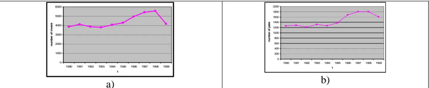
Figure 1 reports the yearly time series of the 44,078 inventors submitting for patents at EPO (1a) and those that are mono–inventors in which case the spatial location of inventors and patents are the same (1b). The selected period 1995–1999 coincides with an evident period of increase in the volume of inventors.

0 1000 2000 3000 4000 5000 6000 1990 1991 1992 1993 1994 1995 1996 1997 1998 1999 t nu m b e r of i n v e n to a) 0 200 400 600 800 1000 1200 1400 1600 1800 2000 1990 1991 1992 1993 1994 1995 1996 1997 1998 1999 t nu m b e r of p a te n b)

Figure 1: (a) Inventors with at least 1 invention and (b) mono–inventors in the period 1990–1999. Source: European Patent Office data processed at CESPRI, Bocconi University, Milan and at the Department of Economics, University of Trento.

With reference to the same dataset Table 1 reports the sectoral distribution of patents with just one inventor in the period 1995–1999. By distinguishing each patent in terms of its specific industrial sector we can interpret our data as a single realization of a multivariate spatial point process. The map reported in Figure 2 displays the overall spatial distribution of the 8279 cases.

Sectors Number of patents (1995–1999)

Electricity Electronics = S1 951

Instruments = S2 831

Chemical Pharmaceutical = S3 675

Process Engineering = S4 1302

Mechanical Engineering Machinery = S5 2830 Consumer goods Civil Engineering = S6 1690

Total 8279

Table 1: Frequency distribution of the number patents with only one inventor distinguished by industrial sector in the periods 1995–1999. Source: European Patent Office data processed at CESPRI, Bocconi University, Milan and at the Department of Economics, University of Trento.

Figure 2: Location of 8279 patents in Italy in 1995–1999. Source: European Patent Office data processed at CESPRI, Bocconi University, Milan and at Department of Economics, University of Trento.

The map reveals a clear agglomeration pattern of the points within some innovative regions, namely Milan’s area in the center–north and the north–eastern part of the country. Indeed, the whole northern regions are very innovative and contain more than 66% of the total number of patents. Conversely the central part of Italy contains only about the 30%, of the patents with a remarkable concentration around Rome and Florence, and only 4% of the patents are located in the southern regions. These empirical findings are not surprising considering the well–known industrial gap existing between Italian regions and, specifically the dualism between the north and the south of the country. Also, the recent literature on knowledge spillovers and specifically the research that concentrated on patent citation (Jaffe et al, 1993; Breschi and Lissoni, 2001; 2006; Driffield, 2006) provides persuasive explanation for the observed geographical pattern. The same kind of information is contained in the graphs reported in Figure 3 displaying the frequency distribution of

inventors (Figure 3a) and the ratio of the number of investors to the number of individuals aged 15 to 65 in 1999 (Figure 3b).

a) b)

Figure 3: Regional distribution of patents in Italy in the period 1995–1999 (a) number of patents (b) patents per 1,000 inhabitants Source: Istat and European Patent Office data elaborated at CESPRI, Bocconi University, Milan and at Department of Economics, University of Trento.

In particular Figure 3b shows that the higher concentration observed in the north cannot be due to population concentration and reveals a genuine prevalence of inventors in that area.

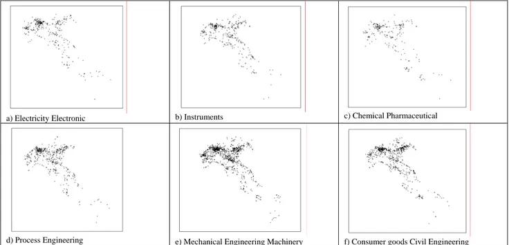
It is helpful to disaggregate the previous map into as many point processes as the number of industrial sectors, each one characterised by a different intensity. To help visualizing this aspect Figure 4 reports the point map for each sector. The same feature of higher concentration in the north appears evident for all 6 sectors considered. Indeed, the observed geographical patterns are very similar for the six sectors with evident concentrations around the main industrial northern towns (Milan and Turin). Some minor, but still evident, concentrations can be observed around Bologna and Venice for patents of the Process Engineering, Mechanical Engineering Machinery and

Consumer goods Civil Engineering sectors and on the east coast between Rimini and Ancona for

the patents of the sector Consumer goods Civil Engineering (see Figure 4f)

a) Electricity Electronic b) Instruments c) Chemical Pharmaceutical

d) Process Engineering _{e) Mechanical Engineering Machinery f) Consumer goods Civil Engineering}

Figure 4: Location of 8279 patents in Italy in 1995–1999 distinguished by sector. Source: European Patent Office data elaborated at CESPRI, Bocconi University, Milan and at Department of Economics, University of Trento.

4.2 Modelling the joint location of patents

In this section we will first of all illustrate with a certain detail the method used for estimating the bivariate K functions. For the purpose of illustrating the estimation method we will concentrate on the spatial interaction between patents of the Electricity Electronics sector and those of the

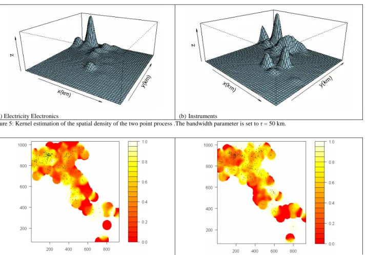
procedures. In order to perform an exploratory analysis of the spatial patterns of points, we initially converted the maps displayed in Figure 4 into spatial densities by using a non–parametric kernel estimator. Figure 5 shows, for the two sectors of Electricity Electronics and Instruments, the kernel density estimation of the random process, say λ

( )

s , s representing the vector of coordinates of the points, s∈ℜ2. For the estimation we considered the following quadratic kernel (see Hastie and Tibshirani, 1990; Fan and Gijbels, 1996):

( )

_∑

< ⎟ ⎟ ⎠ ⎞ ⎜ ⎜ ⎝ ⎛ − = τ τ _{πτ τ} λ j d j d 2 2 2 2 1 3 ˆ s [3]

where τ represents the bandwidth (that is the parameter controlling the smoothness of the surface),

d_l is the distance between point s and the event located at point _sl and the summation refers to all distances d_j < τ.

Interesting insights in terms of exploring the relationships between the two sectors are obtained by superimposing the two maps of points reported in Figures 4a and 4b. In order to do this we exploited the following kernel estimator:

( )

( )

_{( )}

, 1,2 ˆ ˆ ˆ 2 1 ; ; 2 1 ; = = + + i i i s s s τ τ τ _λ λ λ

where both λˆ_τ;i

( )

s and λˆ_τ;1+2

( )

s where computed through expression [3]. We will refer to this kernel estimation as to a dual kernel.

(a) Electricity Electronics (b)Instruments

Figure 5: Kernel estimation of the spatial density of the two point process .The bandwidth parameter is set to τ = 50 km.

(a) Electricity Electronics (b) Instruments Figure 6: Dual kernel estimation of the spatial density. The bandwidth parameter is τ = 35 km.

Figures 6(a) and 6(b) display the output of the estimation procedure obtained for the joint distribution of the Electricity Electronics and Instruments sectors. In particular in Figure 6a we display with a different shading the dual measures ranging from 0 (when there are only patents of sector Instruments) to the value of 1 (in the cases where there are only patents of the Electricity

Electronics sector). A darker shading in Figure 6a reveals the prevalence of patents of the Electricity Electronics sector whereas Figure 6b displays the complementary information for the Instruments sector. In both graphs intermediate values in the scale allows us to identify areas where

both sectors are present. Similar graphs were derived for all other pairs of sectors, but they are not reported here since they do not add particular insights.

Concerning the identification of the bivariate map it seems more grounded the hypothesis of

random labelling with respect to that of independence (see Section 3) in that the labelling of the

patents to a certain sector occurs in a subsequent moment with respect to the moment of the deposit at the EPO. In the remainder of this section we will report the estimation results of the different bivariate versions of the K function that can be used to study the joint location of all pairs of sectors.

To start with, Figure 7 reports the behaviour of the L function for all pairs of sectors. The ∗ effect of co–agglomeration is evident for all sectors at all distances in that all graphs lay entirely above the diagonal which represents the case of random labelling: thus points are more clustered than expected under the null hypothesis of random labelling. In order to investigate more closely this effect of co–agglomeration significant insight can be gained by inspecting the behaviour of the

K cross–functions. In fact, as already said, under the null hypothesis of random labelling we have

that K_ij

( )

t = K_ji

( )

t =K_ii

( )

t =K_jj

( )

t =K

( )

t so that all bivariate K functions (both the auto–functions and the cross–functions) coincide with the univariate K function obtained by merging together the two sectors in one map.

In order to test formally the null hypothesis we need to explicitly choose a functional measuring the departure from the random labelling hypothesis. A first obvious choice is the simple difference between the two functionals ˆ K _ii(t)− ˆ K _jj(t). However, as suggested by Diggle and Chetwynd (1991), such a function can only help in evaluating the clustering of objects and it is less useful when we want to discern the mutual spatial relationships between the two components. A better solution is offered by the differences ˆ K _ii(t)− K_ij*

(t) and ˆ K _jj(t)− K*_ji

(t) that are more informative with respect to the problem in hand. In fact when K ˆ _ii(t)> K*ij(t) and ˆ K _jj(t)> K*ji(t) both patents

labelled i and j display a tendency to spatial segregation within mono–type clusters.

The graphs reported in Figure 8 display the behaviour of the functionals ˆ K _ii(t)− K_ij*(t) and ˆ

K _jj(t)− K*_ji(t) respectively, at the various distances for all pairs of sectors. In all figures we also report the Monte Carlo confidence bands referred to the null H₀2 at a significance level α =0.05. The null hypothesis of random labelling is represented by the horizontal lines in the graphs.7

The visual inspection of Figures 8 suggests in most cases the lack of random labelling, but with remarkably differentiated patterns. First of all, dealing with the joint location of the Electricity

Electronics and Instruments sectors the graphs of the functional Kˆ₁₁(t)−K₁₂* (t) in Figure 8(a) is

7

The critical levels to test the null H02 at 5% significance were obtained as follows. First of all we simulate

1000 =

sim

N maps in which the bivariate vector of the patents is randomized conditionally upon the number of points of Sector i (ni) and of sector j (n ) and upon the coordinates j x of the totaln points (ij nij=ni+n ). Local robust j

estimators (at each distance t) of the upper and the lower limit of the confidence band for the differences Kˆ_ii(t)−K_ij*(t) and Kˆ_jj(t)−K_ij*(t) are then obtained by selecting the

2 α

sim

N and (respectively) the ⎟ ⎠ ⎞ ⎜ ⎝ ⎛ − 2 1 α sim

N order statistics of the 1,000 estimates. The choice of N = 1000 was dictated by Martens et al. (1997) that suggested as a practical rule a sim

always above the K = 0 horizontal line and is above the confidence bands at the 95% confidence level thus indicating significant attraction at all distances. In contrast the graph of the function

) ( ) ( ˆ * 12 22 t K t

K − displays a behaviour that suggests random labelling at small distances (t < 30 km)

with the line falling entirely within the confidence bands at 95% confidence level. Conversely, at higher distances, the graph falls in the lower part of the confidence bands suggesting repulsion between the two sectors.

As a consequence the location of points referring to the two industrial sectors cannot be considered as randomly labelled, rather they display an interesting pattern of attraction–repulsion. The patents of the Electricity Electronics sector tend to locate close to patents of the same sector, whereas patents of the Instruments sector display (at small distances below 30 kilometres) a tendency to locate in the neighbourhood of patents of Electricity Electronics. Such a gravitational effect is dominated by an internal segregation effect (above the mentioned threshold of 30 kilometres) that prevents the patents of the Instruments sector to constitute patches. In summary points of Electricity Electronics tend to cluster on one another while point of Instruments display a repulsion on one another and an attraction towards those of Electricity Electronic. The first effect thus seems to confirms Marshall–Arrow–Romer theoretical expectations (Marshall, 1890; Arrow, 1962; Romer, 1996) and Porter’s idea of dynamical externalities generated by specialization (Porter, 1990), whereas the second effect follows from the dynamic externalities à–la–Jacobs arising from industrial diversification (Jacobs, 1969). By commenting jointly Figures 7 and 8 we observe that the reciprocal aggregation effect between the Electricity Electronics sector and the Instruments sector suggested by the behaviour of the function L12

*

( )

_t

in Figure 7, is not the same in both directions and it is led by the Electricity Electronic sector. From an economic point of view such a results can be easily interpreted by observing that the Instruments sector includes goods whose production requires technologies linked to the Electricity Electronics sector. Thus the knowledge flows generated by firms of the Electricity Electronic sector produce a benefit to the neighbouring industries of the sector of Instruments. In contrast the Electricity Electronics sector includes goods whose production does not require technologies linked to the Instruments sector that most likely benefits from internally generated knowledge flows.

From Figure 8(b) to 8(q) we report the pattern displayed by the functionals ˆ K _ii(t)− K_ij*(t) and ˆ

K _jj(t)− K*_ji(t) in all other pairs of sectors. In order to facilitate the interpretation of such a large amount of information, we can identify four different typologies of attraction–repulsion displayed by the various sectors. A first dominating typology is the one described into details when analysing the Electronic Engineering and Instruments sectors. This pattern is very similar for the pairs of sectors considered in Figures 8(a), 8(c), 8(d), 8(e) (all referring to the relationships between the

Electricity and Electronics sector and the sectors 2, 3, 4 and 5) and 8(f) and, with some differences,

also by Figures 8(l), 8(m) and 8(n) (all involving the Chemical Pharmaceutical sector with respect to Sectors 2, 4, 5 and 6). In this first typology we observe clusters of points of one sector at small distances (between 30 and 50 kilometres) co–existing with points of the second sector that are internally over–dispersed. At high distances points of the second sector become random labelled. Only in the case of Figure 8(m) (depicting the relationships between the sector of Chemical

Pharmaceutical and Mechanical and Civil Engineering) we observe a tendency to cluster after 100

kilometres. It is, however, important to remember that at these higher distances the number of points on which the estimation is based decreases dramatically and thus the estimates are less reliable due to the lack of degrees of freedom. This first typology well describes the stylized facts suggested by Duranton and Overman (2005). A second typology of attraction–repulsion is displayed by the pairs of sectors considered in Figures 8(g), 8(h) and 8(i) involving the relationships between the Instruments sector and the sectors of Process Engineering, Mechanical Engineering

Machinery and Consumer Goods and Civil Engineering. Here the pattern displayed describes

clusters on one sector at small distances (less than 20 kilometres) attracting a second sector which is also self–clustered. At higher distances we conversely observe segregation.

(a) Electricity–Electronics vs. Instruments (b) Electricity–Electronics vs. Chemical–Pharmaceutical

(c) Electricity–Electronics vs. Process Engineering (d) Electricity–Electronics vs. Mcheanical Engineering

Machinery

(e) Electricity–Electronics vs. Consumer goods Civil

Engineering (f) Instruments vs. Chemical Pharmaceutical

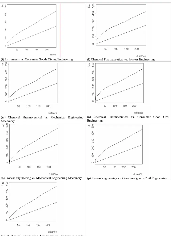
(i) Instruments vs. Consumer Goods Civing Engineering (l) Chemical Pharmaceutical vs. Process Engineering

(m) Chemical Pharmaceutical vs. Mechanical Engineering Machinery

(n) Chemical Pharmaceutical vs. Consumer Good Civil Engineering

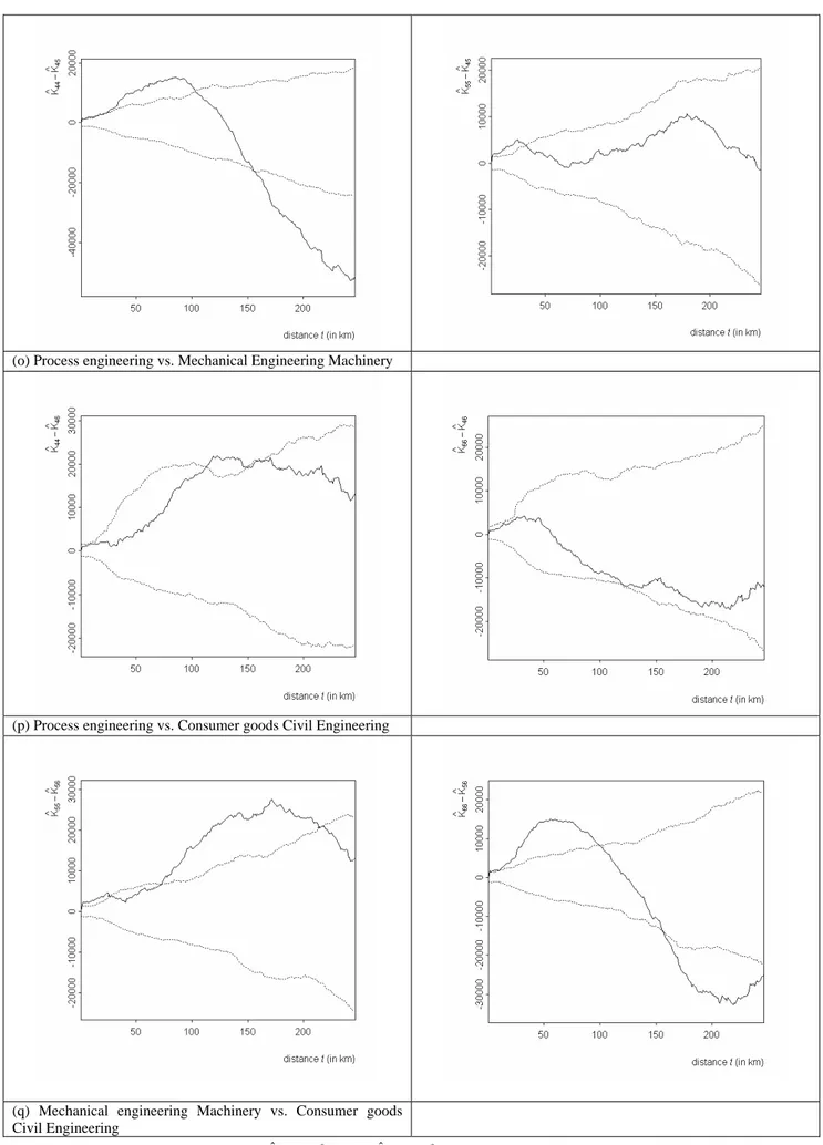
(o) Process engineering vs. Mechanical Engineering Machinery (p) Process engineering vs. Consumer goods Civil Engineering

(q) Mechanical engineering Machinery vs. Consumer goods Civil Engineering

Figure 7: Behaviour of the functional statistics L*ij( )t = Kij*( )t π ∀i,j=1,2,...,6 for all pairs of sectors. In each graph the diagonal represents random labelling. All points above the diagonal represent agglomeration, whereas all points below the diagonal represent repulsion.

(a) Electricity–Electronics vs. Instruments

(b) Electricity–Electronics vs. Chemical–Pharmaceutical

(d) Electricity–Electronics vs. Mechanical Engineering Machinery

(e) Electricity–Electronics vs. Consumer goods Civil Engineering

(g) Instruments vs. Process Engineering

(h) Instruments vs. Mechanical Engineering Machinery

(l) Chemical Pharmaceutical vs. Process Engineering

(m) Chemical Pharmaceutical vs. Mechanical Engineering Machinery

(n) Chemical Pharmaceutical vs. Consumer Goods Civing Engineering

(o) Process engineering vs. Mechanical Engineering Machinery

(p) Process engineering vs. Consumer goods Civil Engineering

(q) Mechanical engineering Machinery vs. Consumer goods Civil Engineering

Figure 8: Behaviour of the functional statistics _Kˆ (_t) _K*(_t) ij

ii − and Kˆjj(t)−Kij*(t) (solid line) and of the corresponding 0.025 and 0.975 quantiles (dashed lines) estimated on the basis of 1,000 simulated random labelling. Reference to causality is represented by the horizontal line.

A third typology is displayed by the pairs of points belonging to the sectors considered in Figures 8(o) and 8(q) that is those referring to the relationships between the Process Engineering sector on one side and the Mechanical Engineering Machiner and Consumer goods Civil

Engineering sectors on the other. Here we notice a tendency to cluster for the points of one sector

which also produces a strong attraction on the points of the other sector. At high distances (more than 150 kilometres) we conversely observe a repulsion in the pattern of the first sector. The effect of concentration of points of the first sector is persistent at all distances in the case reported in Figure 8(q) referring to patents of the Mechanical engineering Machinery sector vs. those of the

Consumer goods Civil Engineering sector.

Finally we have a residual typology where we can classify the exceptions to the typologies previously identified. These are represented by the patterns displayed in Figures 8(b) (referring to

Electricity Electronics vs. Chemical Pharmaceutical) and 8(p) (referring to Process Engineering vs. Consumer goods Civil Engineering). In the first instance we observe clusters of one sector at small

distances co–existing with a second sector that appears to be randomly labelled. In the second instance we have clusters of both sectors only at intermediate distances ranging between 120 and 160 kilometres.

4.3 Controlling for the underlying industrial concentration

The functionals considered in the previous section can help in identifying bivariate clusters of firms, but consider the space as homogeneous with all portions of space having a priori the same probability of hosting a points. Conversely the economic space is highly heterogeneous. On these basis Ellison and Glaeser (1997) suggest that, when looking at the location patterns of firms, the null hypothesis should be that of spatial randomness, but only conditional upon both industrial concentration and overall agglomeration. Their index satisfies this requirement. Similarly Maurel and Sedillot (1999) and Devereux et al. (2004) develop indices with similar properties. Duranton and Overman (2005) notice that “unevenness does not necessarily mean an industry is localized“ and translate these consideration into the formal requirement that “any informative measure of

localization must control for industrial concentration” (p. 1078; see also the Introduction and

Footnote 5). They go further in suggesting that not all points in the space can host a new point and requiring that “the set of all existing sites currently used by a manufacturing establishment

constitutes the set of all possible locations for any point” (p. 1085). In this last section we wish to

introduce the use of the bivariate K functions to fulfil Ellison-Glaeser requirement and we compare for each sector the actual pattern with the pattern generated by all patents considered as a whole. More in details we compute the differences between the bivariate K function for each sector on one side and the univariate K function computed considering all sectors together. Such a difference can help in identifying sectors that are over–concentrated (over–dispersed) not in absolute terms as in the traditional univariate K analysis (Marcon and Puesch, 2003a), but conditionally upon the spatial pattern displayed by the other firms for the economy as a whole. Of course we are aware that, for this analysis to be complete, we should consider the spatial pattern of all firms in the economy, but in the empirical analysis reported here we restrict ourselves to only the pattern of patents included in the EPO database to have at least some indications.

The results of this analysis are reported in Figures 9(a) to 9(f).

The exam of Figures 9 reveals some interesting features. First of all the patents of the

Electricity Electronics and Chemical Pharmaceutical sectors display over–concentration with

respect to the underlying global concentration of patents at all distances (see Figures 9(a) and 9(c)). In particular Electricity Electronics presents high and increasing concentration up to 80 kilometres whereas Chemical Pharmaceutical presents the maximum concentration at around 60 kilometres and then a decreasing pattern and even randomness after 160 kilometres. Such results parallel those of Duranton and Overman (2005) that found localization mostly at small scales (less than 60 kilometres) and a general tendency for Chemical Pharmaceutical products to over–clustering.

(a) Electricity Electronics

(b) Instruments

(c) Chemical Pharmaceutical

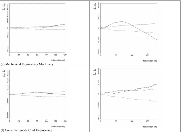
(e) Mechanical Engineering Machinery

(f) Consumer goods Civil Engineering

Figure 9: Behaviour of the functional statistics Kˆit(t)−Ktt*(t) and Kˆtt(t)−Kti*(t) (solid line) and of the corresponding 0.025 and 0.975 quantiles (dashed lines) estimated on the basis of 1,000 simulated random labelling. Reference to causality is represented by the horizontal line. Points above the 0.975 quantiles denote significant agglomeration of points of one sector around points of all other sectors. Points below the 0.025 quantiles denote significant repulsion of points of one sector from points of all other sectors.

Secondly, the Instruments sector displays over–dispersion with respect to the underlying distribution of patents at distances greater than 50 kilometres. Thirdly, the patents of the Process

Engineering sector display a more complex pattern with significant over–clustering only in the

interval between 70 and 140 kilometres. Finally the Mechanical Engineering Machinery and the

Consumer goods Civil Engineering sectors display random labelling at all distances (remember that

estimates at high distances are less reliable due to the lack of degrees of freedom). Therefore in these two sectors there seems to be no specific tendency to either clustering of repulsion apart from those that are characteristic of the economy as a whole.

5. Summary and concluding remarks

In this paper we extended the use of Ripley’s K functions (Ripley, 1977) previously considered in the economic literature by Arbia and Espa (1996), Quah and Simpson (2003) Marcon and Puesch (2003a) and Duranton and Overman (2005) to the analysis of the joint spatial pattern of industries.

By applying a methodology based on the bivariate cross-functions K to the spatial distribution of patents in Italy in the period 1995–1999, we have been able to discern quite distinct geographical patterns for the six sectors considered.

Our main findings are the following:

• The pattern displayed by the patents of all pairs of the six sectors considered is always of agglomeration when analysed in absolute terms looking at the standard bivariate K functions.

• However, when looking more closely at the pair–wise relationships between the six sectors considered, a more differentiated situation emerges. In fact, most of the observed joint patterns (precisely 8 of the 15 pairs of sectors considered) display a situation of dominance of one sector on the other. This dominance assumes that there is a leading sector that is clustered in space at small distances (up to 50 kilometres) and a second sector that is dispersed internally and clustered around the leader. In particular this is the pattern displayed by the patents of the Electricity Electronics and the Chemical

Pharmaceutical sectors that act as leaders with respect to the other sectors.

• Such a specificity of the Electricity Electronics and the Chemical Pharmaceutical sectors emerges also when considering the analysis of agglomeration conditional on the global concentration of patents in the economy as a whole. In fact, in this case, the mentioned sectors are the only two that present over–clustering with respect to the general pattern of all patents. In particular we notice a climax at around 80 kilometres for the patents of the Electricity Electronics sector and at around 60 kilometres for the patents of the Chemical Pharmaceutical sectors. Conversely for the patents belonging to the other sectors we record over–dispersion for the Instruments sectors and no significant departure from randomness in the remaining sectors.

The analysis considered here has shown the importance, but also the limits of a static approach and the necessity to introduce temporal dynamics in order to reconstruct the whole process of individual choices behaviour. Thus an important step forward in the application of the spatial econometric techniques discussed here is represented by the introduction of the time dimension. In fact the analysis of the static bivariate K functions registers only the situation in one definite period of time and provides only a single snapshot of the whole dynamic process. Quite obviously, this snapshot can be of help in suggesting the generating mechanism of individual locational choices as it is realized in a dynamic context like a single photogram reveals something about the nature of the movie it is drawn from. For instance, the individual choice behaviour of firms suggested by Figures 8 (a) could be interpreted as the process through which in a first moment industries of one sector (say Type 1) locate themselves in the space at random and industries of another sector (say Type 2) tend to locate around them to exploit technological and physical spill–overs. If new Type 1 industries locate in the area, they tend to locate away from Type 2 industries creating a buffering zone that can be due to physical or economical constraints. This behaviour seems to suggest a leading position of Type 1 industries with respect to Type 2. This dynamic, however, describes only one of the possible behaviours, and more refined spatial laws of motion could be suggested by the analysis of proper dynamic K functions.

The theoretical basis for considering dynamic spatial patterns in economic analysis are well depicted by Quah and Simpson (2003). Dynamic “space–time” K–functions (Diggle, 1993; Diggle

et al., 1995) can be conceived as functionals depending on both spatial distances and the time lag

which indicate how many points characterized by a certain label fall within a certain distance of other points after a certain period of time. Such an analysis would greatly help the study of the concentration of industries and the analysis of diffusion processes which, in turn, are issues of tremendous importance when analysing sectoral growth and the rise and fall of regions within one country. Since understanding the dynamics of the spatial distribution of firms can also help to clarify the complex mechanisms of international trade, the development of this field appears to be as one of the most challenging in the future research agenda.

References

Acs, Z. J., Audretsch, D. B. and Feldman M. P. (1994) R&D Spillovers and Recipient Firm Size. The Review of Economics and Statistics 76(2): 336–340.

Arbia G., Copetti M. and Diggle P.J. (2006) Modelling individual behaviour of firms in the study of spatial concentration, in U. Fratesi L. and Senn (eds.) Growth in Interconnected

Territories: Innovation Dynamics, Local Factors and Agents, Springer−Verlag (forthcoming). Arbia, G. (1989) Spatial data configuration in regional economic and related problems, Kluwer Academic publishers, Dordrecht.

Arbia, G. (2001) Modelling the geography of economic activities in a continuous space, Papers

in Regional Sciences, 80, 411–424.

Arbia, G. (2006) Spatial Econometrics: with applications to regional convergence, Springer– Verlag, Berlin.

Arbia, G. and Espa, G. (1996) Statistica Economica Territoriale, Cedam, Padua.

Arrow K.J. (1962) The Economic Implications of Learning by Doing. Rev.Econ.Studies: 155– 73.

Audretsch, D. B. and Feldman, M. P. (1996) R&D Spillovers and the Geography of Innovation and Production. The American Economic Review, 86(3): 630–640.

Bairoch, P. (1988) Cities and Economic development: From the Dawn of History to the present. Chicago Press.

Barnard G.A. (1963) Contribution to the discussion of Professor Bartlett’s paper, Journal of the

Royal Statistical Society, B, 25, 294.

Besag J. (1977) Contribution to the discussion of Dr. Ripley’s paper, Journal of the Royal

Statistical Society, B, 39, 193–195.

Besag J. and Diggle P.J. (1977) Simple Monte Carlo test for spatial pattern, Applied Statistics, 26, 327–333.

Breschi S. and Lissoni F. (2001) Knowledge spillovers and local innovation systems: A critical survey, Industrial and Corporate Change, vol. 10 (4): 975–1005

Breschi S. and Lissoni F. (2006) Cross–firm inventors and social networks: localised knowledge spillovers revisited”, Annales d’Economie et de Statistique (forthcoming).

Ciccone A. and Hall, R. R. (1996) Productivity and the density of economic activity, American

Economic Review, 86, 1, 54–70.

Cliff A. D., and Ord, J. K. (1981) Spatial processes: models and applications, Pion, London. Devereux, M. P., Griffith R., and Simpson H. (2004) The geographic distribution of production activity in the UK, Regional Science and Urban Economics, 34, 533–564.

Diggle P.J. (1983) Statistical Analysis of Spatial Point Patterns, Academic Press, New York. Diggle P.J. (1993) Point process modelling in environmental epidemiology, in V. Barnett and K.F. Turkman (eds) Statistics for the environment, John Wiley, Chichester.

Diggle P.J. and Chetwynd A.G. (1991) Second−order analysis of spatial clustering, Biometrics, 47, 1155–1163.

Diggle P.J., Chetwynd A.G., Haggkvist R. and Morris S. (1995) Second–order analysis of space−time clustering, Statistical Methods in Medical Research, 4, 124–36.

Dixon P.M. (2002) Ripley’s K function, in A.H. El–Shaarawi and W.W. Piegorsch (eds.)

Encyclopedia of Environmetrics, Volume 3, John Wiley & Sons, Chichester, 1796–1803.

Driffield N. (2006), On the search for spillovers from Foreign Direct Investment (FDI) with spatial dependency, Regional Studies, 40, pp. 107-119.

Duranton, G., and Overman H. G. (2005) Testing for localisation using micro–geographic data,

Review of Economic Studies, 72, 1077–1106.

Ellison, G. and Glaeser E. L. (1997) Geographic concentration in U.S. manufacturing industries: A dartboard approach, Journal of Political Economy, 105(5), 889–927, October.

Fan, J. and Gijbels, I. (1996). Local Polynomial Modelling and Its Applications. Chapman and Hall, London.

Fujita, M., Krugman, P. and Venables A. (1999) The Spatial Economy: Cities, Regions, and

Gatrell A.C., Bailey T.C., Diggle P.J. and Rowlingson B.S. (1996) Spatial point pattern analysis and its application in geographical epidemiology, Transactions of the Institute of British

Geographers, 21, 256–274.

Glaeser, E. L., Kallal, H. D., Scheinkman, J. A. and Schleifer, A. (1992) Growth in Cities.

Journal of Political Economy, 100 (6): 1126–1152.

Goreaud F. and Pélissier R. (1999) On explicit formulas of edge effect correction for Ripley’s

K−function, Journal of Vegetation Science, 10, 433−438.

Goreaud F. and Pélissier R. (2003) Avoiding misinterpretation of biotic interactions with intertype K₁₂

( )

t −function: population independence vs. random labelling hypotheses, Journal of

Vegetation Science, 14, 681–692.

Griliches, Z. (1979) Issues in Assessing the Contribution of Research and Development to Productivity Growth, Bell Journal of Economics 10: 92–116.

Haining R. P. (2003) Spatial Data Analysis – Theory and Practice, Cambridge University Press, Cambridge.

Hastie, T. and Tibshirani, R. (1990). Generalized Additive Models. Chapman and Hall, London. Henderson, J. V. (2003) Marshall's scale economies, Journal of Urban Economics, 53(1), 1–28, January.

Henderson, V, A. Kunkoro, M. (1995) Turner, Industrial development of cities, Journal of

Political Economy ,103: 1067–1090.

Ioannides, Y. M., and Overman H. G. (2004) Spatial evolution of the US urban system, Journal

of Economic Studies, 4, 131–156.

Jacobs J. (1969) The Economy of Cities, Random House.

Jacobs J. (1984) Cities and the Wealth of Nations: Principles of Economic Life. New York: Vintage

Jaffe, A. B. (1989) Real Effects of Academic Research. The American Economic Review, 79(5): 957–970.

Jaffe A. B. and Trajtenberg, M. (1996) Flows of Knowledge from Universities and Federal Laboratories: Modeling the Flow of Patent Citations Over Time and Across Institutional and Geographic Boundaries, Proceedings of National Academy of Science, vol. 93, pp. 12671–12677.

Jaffe A. B. and Trajtenberg, M. (2002) Patents, Citations and Innovations: A Window on the

Knowledge Economy. Cambridge: MIT Press.

Jaffe A. B., Trajtenberg, M. and Fogarty, M. (2000) The Meaning of Patent Citations: Report of the NBER/Case Western Reserve Survey of Patentees, NBER working paper No. 7631.

Jaffe, A. B., Trajtenberg, M. and Henderson R. (1993) Geographic localization of knowledge spillovers as evidenced in patent citations, Quarterly Journal of Economics, 108(3), 577–598, August

Krugman, P. (1991) Geography and Trade (Cambridge: MIT Press)

Kulldorff M. (1998) Statistical methods for spatial epidemiology: test for randomness, in A. Gatrell and M. Löytönen (eds.) GIS and Healt, Taylor & Francis, London, 49–62.

Lotwick H.W., Silverman B.W. (1982) Methods for analysing spatial processes of several types of points, Journal of the Royal Statistical Society, B, 44, 406–413.

Lucas, R. E. (1988) On the mechanics of economic development. Journal of Monetary

Economics, 22(1): 3–42.

Marcon, E. and Puech, F. (2003a) Evaluating Geographic Concentration of Industries Using Distance–Based Methods, Journal of Economic Geography, 3(4): 409–428.

Marcon, E. and Puech, F. (2003b) Generalizing Ripley’s K function to inhomeogeneous

populations, mimeo.

Marshall A. (1890) Principle of Economics. Macmillan, London

Maurel, F. and Sedillot, B. (1999) A measure for geographical concentration of French Manufacturing industries, Regional Science and Urban Economics, 29, 5, 575–604.

Porter M.E. (1990) The Competitive Advantage of Nations. New York: Free Press Quah D. and Simpson H. (2003) Spatial Cluster Empirics, mimeo.

Rauch, J. E. (1993) Productivity gains from geographic concentration of human capital: Evidence from the cities, Journal of Urban Economics, 43(3), 380–400, November

Ripley B. D. (1976) The second–order analysis of stationary point processes, Journal of Applied

Probability, 13, 255–266.

Ripley B. D. (1977) Modelling Spatial Patterns (with discussion), Journal of the Royal

Statistical Society, B, 39, 172–212.

Ripley B. D. (1979) Test of ‘randomness’ for spatial point pattern, Journal of the Royal

Statistical Society, B, 41, 368–374.

Romer P.M. (1986) Increasing Returns and Long–Run Growth, J.P.E. 94: 1002–37.

Yule, G. U. and Kendall, M. G. (1950) An introduction to the theory of statistics, London, Griffin.

! " # $ % " ! " & ! ! ' ( ! ) * + , * - -. / # ! - . ! 0 - ) # ! ! $ 1 / 1 % & + 0 ' # ! . / # " ( ) * % & $ 2 ) ! " 1 % . % 1 # ! " / / ' ! * ' ! % ( ! ) $ ) $ 3 4 5 4 5 . ! % & 1 6 ( ( ( 7899 789: $ %

' ($ 0 ( ; < $ $ = + 1 . % 1 . + , $ - . 1 0 ! " ! = $ + . / 0* $ + . / 1 1 ( - . % +2 3 - 4/ # $ % & 1 # 3 - . - ( 5 6 $ ' 1 ! ) . ' + 2 + " * . ' . ! * - 7 8 ) 9 . ' 0 + ' * . 7 8 ) : ' $ " ) / " % ) = ! " 0 ! " 1 > ! " &" " 6 $ " ' %-* & ' * # - #- -$ + 2 /

& * 1 ' ' . 7 ) ) ' 1 % / ! . ) 7 ) * 2 ) + + ?, ( @ 1 ' 1 ) 7 ) 9 1 > 1 $ 44 . : ) " 1 ) * # ! - ' '- .0 ! ' & ?* /@ 6 A ! . - ' '- .0 ! ' & ?* //@ ' ! . ( # ! - , .> - & % ' ! . . 4 1 ' , * 3 ' ! $ $ ! . & 1 0 0 ! " & . 6 - - . 4 . - / & 3 ! 0 ( ) . 3 ( # & ( # + " ! " & & $ $ / 4 & ' * # ! ) ; % < % #- - $

& * 2 1 ! ' 1 - ( (/ . 1-. 7BB ' #- - $ , + 3= & 9 ' ( ) ' # - ' * #- - $ + 2 / & : 3 &#* 0 + 2 / & % $ $ & / $ " & ' 4.0 & 5 .0 / ! . % & 1 ' & .> 1 7 ) ) & 1 / . 1 * ' 0 . 7 ) ) & & ! $ , ! ' -& 7 ) ) & ' > " / # $ 8 - 7 ) ) & * * ! # 3 -1 ) 3 . 4 # % " & 9 ' ! " & : % 4 / - .$" - / 4 $ 44 $ " & - . ( . / & + ) . 4 . - / ' 3 C3 - - " . . 4 # % +

' 6 ) ) / ' 1 +2 3 - 4/ ' ) - * -* , 3 ' & + ' ! ) * ' * ' ' - #- -$ ' ' ! $ & # . % %- D ' . ' * 2 ( / .0 . 3 "4 34 . ' 9 $ ( E . ? - - 4 ? -- 4 - 4 ! . ' : ! 4 5" / & $ " * 1 ( # 1 ! * ' ) * - ! . F ' / 7 8 ) * + 1 ' ! . 7 8 ) * , ' ' 6 . ! % ! . * & $ + $ @