MODELLING PREVENTION STRATEGIES IN PUBLIC
HEALTH
Giuseppe Schinaia1
Department MEMOTEF, Sapienza University of Rome, Rome, Italy Valentino Parisi
Department of Economics and Law, University of Cassino and Southern Lazio, Cassino, Italy
1. Introduction
Health is widely acknowledged as an economic good representing a pre-requisite for individual well-being and economic productivity. Public policy actions which focus on health promotion and improvement are essential for sustainable economic welfare, and prevention measures are often the key to successful health policies.
From a theoretical standpoint, health prevention belongs to the category of pure public goods to which the properties of non-rivalry and non-excludability apply. Furthermore, health promotion programs entail a long-term distribution of the benefits that make them less profitable to private firms. It is, therefore, the public sector which is mostly responsible for developing prevention programs: sound tools for cost reductions and resource management are becoming more and more crucial in the long-term perspective under increasing public budget con-straints.
As early as the 1980s, prevention issues were already under study via general schemes of cost-effectiveness, cost-benefit and related analyses (see for instance Torrance, 1986 and Birch, 1987) while a more exhaustive economic analysis is relatively new (Haddix et al., 2003). At the same time operational approaches to prevention strategies and application tools to support policy making were being developed to face various organizational constraints: extensive discussion can be found in (Teutsch, 1992). However, only a few studies still examine the impact of prevention on public health expenditure in a comprehensive model-theoretical framework, as in Haddix et al. (2003); Davies et al. (2003) and Mackinnon and Dwyer (1993).
Furthermore, several studies provide evidence of the positive impact of health promotion on relevant economic variables (labour supply, productivity, wages and earnings: for a review see Suhrke et al., 2005). International organizations, public
health authorities and researchers have particularly evaluated prevention measures in public health alerts, such as wide-spread epidemics, life styles, and the erad-ication of endemicities (Boily et al., 2007; Goldie et al., 2006; Zethraeus et al., 2007; Kaestner et al., 2014). Following a thorough analysis of their impact, large scale programs against obesity and measles were launched by both the O.E.C.D. (2009) and the W.H.O. (2011), and their outcomes have formed the object of var-ious studies (Waters et al., 2011). Similarly, Zhou et al. (2005) have extensively evaluated the public health savings of childhood routine immunisation campaigns in the US.
As for the various types of prevention that can be implemented on a spe-cific population of reference, Boland and Murphy (2012) remark that “primary prevention blocks or delays the onset of disease, avoiding direct costs associated with diagnosis, treatment, rehabilitation and indirect costs associated with lost function, lost work productivity and other societal costs. Secondary prevention includes the early detection of disease e.g. through screening. Tertiary prevention services act when a disease or injury is already present, and seek to limit the effect of the condition and to improve quality of life, e.g. chronic disease management programmes”.By far, secondary prevention studies are more common in the liter-ature. Studies in cancer prevention have been conducted by Holland et al. (2006); Sasieni et al. (2009); Duffy et al. (2010) and by the Medical Center Expert Group (2011) of the Vrije Universiteit in Amsterdam, while Sassi and Hurst (2008) offer a comprehensive analysis of the socio-economic effects of the prevention of life-style related chronic diseases. As for primary prevention,using a decision-analytic model, Cipriano et al. (2007) estimate the cost gains achieved by screening at birth campaigns.
As prevention measures are implemented more widely and at the same time the globalization of pathologies has placed higher pressure on public health budgets worldwide, there is a growing urge to implement cost-reducing strategies where prevention measures play a major role. However, policy makers need comparable, easy to use and reliable planning tools to schedule interventions and evaluate their impact. As clearly explained in Goldie (2003): “No clinical trial or single cohort study will be able to simultaneously consider all of these components. Cost-effectiveness analysis and disease-simulation modelling, capitalizing on data from multiple sources, can serve as a valuable tool to extend the time horizon of clinical trials, to evaluate more strategies than possible in a single clinical trial, and to assess the relative costs and benefits of alternative policies to reduce mortality”.
This paper offers an original and overall modelling approach to designing pri-mary and secondary prevention measures under an essentially budget-management perspective. Based on its demographic structure and a disease epidemiology, a reference population and a multistate distribution of pre-clinical, asymptomatic conditions among affected individuals is here considered.
Section 2 presents a simple primary prevention model and expands it to a multistate, secondary prevention evaluation model. Section 3 further analyses qualitative features of the model and its mathematical relationships to variable prevention policies. Next, in section 4 a review of the most recent statistical devel-opments is presented with specific reference to the model parameters and in 5 an
application to overall Italian cancer data is offered,along with further extensions of the general model to include more complex schemes, such as disease preva-lence instability and differential survival experiences. Conclusions and material for further developments are in section 6.
2. General prevention models
As remarked in the previous section, primary and secondary prevention measures act at different population/disease levels and interactions. In this section preven-tion evaluapreven-tion schemes for primary and secondary intervenpreven-tions will be presented with regard to expenditure and savings obtained by a public health system, with-out a selection in the admission of the affected individuals to treatment (i.e., all affected individuals have equal access to clinical treatment). Furthermore,the dis-ease prevalence in absence of prevention interventions is supposed to be stable and constant over the time horizon considered; the consequences for dropping this hypothesis will be briefly analysed in section 5, where possible extensions of the model will be described.
A simple scheme of primary interventions may be thought of as an information campaign directed at the general population or at a sorted proportion of it. This roughly involves per capita expenditure and results in a reduction of the disease incidence and prevalence, at variable levels, corresponding to the efficacy of the campaign.
Let P = p + ¯p be the total number of individuals in a population, divided into p = βP individuals that will eventually become affected by some disease under study (β being the known prevalence of the disease in the general population) and ¯
p = (1− β)P individuals that will not develop the disease.A public health system that must treat all affected individuals has a predictable, total, disease-related cost C given by
C = A0+ Ap (1)
where A0 is a general fixed system cost and A is the variable treatment cost per
affected individual.
Thus, given a per capita prevention expenditure e and a corresponding propor-tion γ of individuals positively responding to the prevenpropor-tion measures, the total cost (1) becomes
ˆ
C = A0+ A(1− γ)p + eP (2)
Note that the term P does not include already affected individuals, as they are not the object of the prevention actions and are, therefore, included in the fixed cost term A0.
Using (1) and (2), a system saving is thus attained if
S = C− ˆC = Aγp− eP > 0 ⇒ e < Aγβ (3) which provides an exact evaluation of the profitability of a prevention investment: in fact, this turns out to be economically profitable only when the variable treat-ment costs and/or the disease prevalence are high enough to compensate for the prevention costs.
A more complex modelling scheme is to be used to evaluate secondary preven-tion measures as these intervenpreven-tions aim at different results and involve various, disease-related types of individuals. In this case the reference population includes those already affected individuals at asymptomatic, pre-clinical stages, aiming at an early detection of the disease and at its early treatment Simeonsson (1991).
Let the total population be given by P = p+ ¯p with p asymptomatic individuals already affected by the disease under study at n increasing levels of severity, and ¯
p healthy individuals, and let βi i = 1, . . . , n be the known prevalences of each level of severity of the disease in the population.
Similarly to (1), the public health system in absence of prevention measures has a predictable, total, disease-related cost C given by
C = A0+
n ∑
i=1
αiβiP (4)
where A0is a general fixed system cost, and αi, i = 1, . . . , n are the variable
treat-ment costs per affected individual and related to the n levels of disease severity. Note that the distribution of individuals in (4) is supposed to be induced by the disease symptomatology: i.e., affected individuals enter the cost function (4) at a level corresponding to detectable symptoms.
Possible prevention measures can be thought of as some form of screening over the entire population P to detect all affected individuals before their disease becomes symptomatic (i.e., at a lower level of severity). Let e be the unit cost of the prevention operations; the total cost of prevention is therefore given by
eP = e ( n ∑ i=1 βiP + ¯p )
and the prevention cost per affected individual actually detected is then given by ε = e∑nP i=1βiP = e ( 1 ∑n i=1βi )
The effects of prevention on the number of affected individuals are thus given by their redistribution among the n levels of severity (with the corresponding changes in the treatment costs) according to a lower triangular transition matrix ∏
=⌊πij⌋i;j=1,...,n such that: n
∑ i=j+1
πij≤ 1 and πij = 0 i < j 1−∑ni=j+1πij i = j πij i > j (5)
where the underlying hypotheses are:
• the disease prevalence does not change within the time horizon considered, • prevention measures do not interact with the symptomatology of the disease
(i.e., the level of severity detected by prevention measures cannot be higher than the level corresponding to detectable symptoms).
By using (4), the total system cost, when prevention measures are put in place, is thus given by ˆ C = A0+ n ∑ i=1 αiβiP + n∑−1 i=1 n ∑ j=i+1 αiπjiβjP− n ∑ i=2 i−1 ∑ j=1 αiπjiβiP + ε n∑−1 i=1 n ∑ j=i+1 πjiβjP (6) where the variable treatment cost of the i-th level of severity is now given by the algebraic sum of
• αiβiP : the cost of individuals detected at symptomatic level of severity;
• ∑nj=i+1αiπjiβjP : the cost of individuals detected at the i-th level of severity
with a higher symptomatic level of severity;
• ∑ij=1−1αiπijβiP : the cost of individuals with i-th symptomatic level of sever-ity detected at a lower level of seversever-ity;
• ε∑nj=i+1πjiβjP : the prevention costs per individual with i-th symptomatic
level detected at a lower level of severity. A system saving is thus attained if
S = C− ˆC > 0 which, by using (4) and (6), becomes
− n∑−1 i=1 n ∑ j=i+1 αiπjiβj+ n ∑ i=1 αiβi i−1 ∑ j=1 πij− ε n−1 ∑ i=1 n ∑ j=i+1 πjiβj> 0
By using some simple algebra and solving for ε we have
ε < n∑−1 i=1 n ∑ j=i+1 (αj− αi)πjiβj n∑−1 i=1 n ∑ j=i+1 πjiβj (7)
Thus an economically sound prevention policy can be effectively set up when the cost of one asymptomatic detected individual is smaller than the average cost re-duction, weighed by the newly detected prevalences of each level of severity. In the absence of further, specific information on the morbidity of the disease under study at various levels of severity (i.e., no direct or indirect information avail-able on the πji terms), the assumptions that the whole population P undergoes the prevention screening, and that no biased error occurs during the screening operation, provide a reasonable ground to the conservative hypothesis that the prevalence rates βii = 1, . . . , n of the general population also apply to the various levels of severity. This implies that all transitions πij can be approximated by the
corresponding prevalence rates βj ∀j > i, i = 1, . . . , n and, similarly to (3), (7) can be expressed in terms of the unit cost e of prevention operations and becomes
e < n∑−1 k=1 βk n−1 ∑ i=1 n ∑ j=i+1 βiβj n−1 ∑ i=1 n ∑ j=i+1 (αj− αi)βiβj (8)
Under the hypothesis of non-decreasing costs between the disease stages and the trivial remark that βi > 0 for at least two different i’s, i = 1, . . . , n, then e ≥ 0∀αii = 1, . . . , n and e = 0 if and only if αj− αi = 0∀j > i i, j = 1, . . . , n.
3. Qualitative Analysis
Some further insight into the modelling approach in the previous section is pro-vided by a thorough analysis of (8).
By defining the vectors β = [βi]i=1,...,n and α = [αi]i=1,...,n and the Hollow matrix B1= 0 −β1 −β1 −β1 · · · −β1 β2 0 −β2 −β2 · · · −β2 β3 β3 0 −β3 · · · −β3 β4 β4 β4 0 · · · −β4 · · · · · · βn βn βn · · · βn 0 where In is the n× n identity matrix, (8) can be re-written as
e <−2 l ′ nβ tr(B2 1) α′B1β or e <−2 l′nβ tr(B2 1) α′B2ln (9)
where ln is the n-vector with elements all equal to 1’s and B2= B1Inβ. Vectors α, β and ln in (9) represent, respectively, the treatment cost profile of the disease under study, the prevalence profile and the profile of an unscreened individual; therefore, the degenerate, bilinear forms in (9) map, respectively, a prevalence profile and an unscreened individual onto the cost space and the degenerate con-dition accounts for the reduction of the space dimensionality as from (5).
Let us now define the upper limit in (9) as
f (β) =−2 1
′nβ
tr (B2 1)
α′B21n (10)
Its derivatives with respect to each component of β provide a qualitative evaluation of the per capita expenditure threshold for secondary prevention measures, as explained in the previous section. While it is not reasonable to assume any direct intervention on the disease progression, various forms of primary prevention can, however, be implemented to actually reduce the disease incidence, which, in the
long run, results in a decrease of β1. Using some straightforward vector calculus, we have that df (β)dβ 1 can be expressed as df (β) dβ1 = g1(α; β)− g2(α; β) (11)
where the domain of g1 consists of the (n− 1) differences (αi− α1) and of all
βi∀i = 1, . . . , n while the domain of g2consists of the remaining (n−2)! differences
(αi− αj) for i > j and of βi ∀i > 1.
When n = 3, (11) can be explicitly written out as df (β)
dβ1
= [β2(α2− α1) + β3(α3− α1)]
× (β2
1β2+ β12β3+ 2β1β2β3+ β22β3)− β23β3(α3− α2) (12)
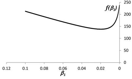
With reference to (12) and for selected values of β2, β3 and α the graph of f (β)
as a scalar function of β1 is presented in figure 1, the change of its curvature
corresponding to the solution of df (β)dβ
1 = 0. 0 50 100 150 200 250 0 0.02 0.04 0.06 0.08 0.1 0.12
f(
E
1)
E
1Figure 1 – Graph of f (β) from (10) as a scalar function of β1
It is thus evident that both g1 and g2 are non-negative and non-decreasing over
their whole domains. Under general conditions, g1≥ g2 and (10) increases;
how-ever, when the disease entry level prevalence β1 decreases (by some forms of
pri-mary prevention or other public health interventions) below the value where (11) vanishes, then the allowance for secondary prevention expenses starts increasing, due to the prevailing cost reductions of the diagnosed cases.
4. Statistical Remarks and Parameter Evaluation
Although the objective of the present paper is to illustrate the basic features of the proposed prevention model, some statistical remarks might be of help to
understand the global functioning of the system and the model building process. The schemes (4) and (6) presented above are both based on a first order ap-proximation of an underlying compartmental system Jacquez (1996) of the health care costs among the various levels of severity of the pathological status under study. This amounts to limiting the model scheme to some specific time instant t0
(i.e., when no dynamic evolution is involved). A further,dynamical development of this scheme will be the object of future research and is therefore here excluded from these statistical remarks.
In the next, two main questions will be briefly addressed, as the evaluation of the fractional transfer coefficients (FTC, see Jacquez and Simon, 1993, for a thorough theoretical overview) involved in the compartmental transitions can be performed using various techniques, while more statistical details can be drawn from the specialized literature, using both standard and ad hoc methods.As shown in Schinaia (1999), all compartmental models have a topological structure of their FTC parameter space which, in turn, leads to a dynamical evolution of the model output. When, as in (4) and (6), the underlying compartmental structure of the model presents no dynamical evolution then the model output estimates C and
ˆ
C can be regarded to as a pointwise picture of the functioning system at some t0
and dependent on the vectors α and β.
In turn, α and β are to be externally determined by available longitudinal data sets, by selecting appropriate covariates of known significance to the pathological status under study and by usually fitting some forms of regression model. However, more specific calculation reduction and covariate selection techniques have been developed in the past years; artificial neuronal networks (Gambhir et al., 1998), ROC curves (Heagerty and Zheng, 2005 and Krzanowski and Hand, 2009) and their extensions (Hand, 2009) and genetic-type algorithms (Santhoji Katare et al., 2004) are among the most recent methods to determine accurate evaluations when missing or incomplete data are present.
5. Applications and Extensions
As illustrations of the use of the prevention model presented in the previous sec-tions, a numerical application to Italian global tumor data and two extensions of the mathematical framework are here presented.
The various tumor forms are a typical example suitable to most of the mod-elling hypotheses as in section 2; even when limited to any incidence sub-populations, these may, however, be easily detected (male-female, for instance). In the follow-ing simple numerical examples of prevention schemes are based on the model in the previous section and use cancer treatment- and cost-data from heterogeneous, external studies.
In order to implement the model extensions it must be noted that the vector setting of the prevention expenditure limit (9) may be effectively used, by di-rect modifications of α, β and 1n, to accommodate complex prevention schemes, such as the selection of differential survival sub-populations and communicable (infectious or hereditary) diseases.
TABLE 1
Unit treatment costs and prevalence by tumor primary site Primary Prevalence (%)* Unit cost (×1000e)**
Lung 0,17 36 Stomach 0,12 19 Melanoma 0,27 21 Colon/Rectum 0,69 24 Cervix 0,05 10 Breast 2,26 17 Prostate 1,23 19 Leukemias 0,09 77
* A.I.R.TUM. – Tumors in Italy (2012) - http://www.tumori.net ** CENSIS, from Economist Intelligent Unit (2010)
5.1. An Application to Italian Cancer Data
Italian prevalence and global unit cost data corresponding to various primary tumor sites are shown in Table 1.
While no staging data are required in this simplified application of the primary prevention scheme as from (3), the secondary prevention scheme requires cost and prevalence distribution data for the application of (8). For the sake of homogene-ity of the various primary tumor sites and in order to outline the use of the model, the staging classifications have been reduced to 3 for each type of tumor on the basis of epidemiological and clinical data drawn from the existing medical litera-ture. However, as the detailed cost distribution at each stage is not immediately available,a cost proportionality hypothesis was applied to the data in Table 1 and the resulting expenditure limits were computed according to (8).
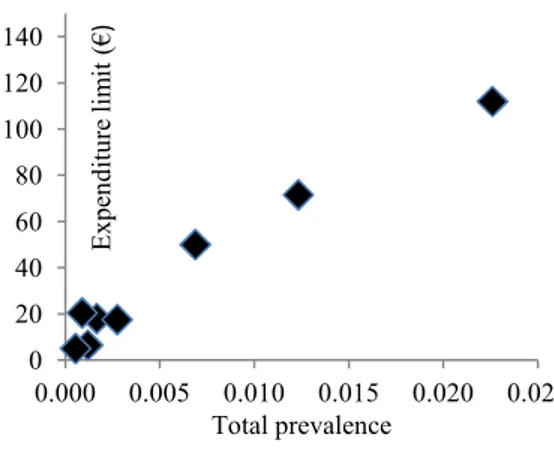
Figures 2 and 3 show two examples of primary prevention schemes where: the expenditure limits are mapped against the corresponding total prevalences, and the expenditure limits are mapped against the total unit treatment costs.
A visual inspection of figures 2 and 3, shows that the secondary prevention expenditure limit is approximately linearly correlated to the pathology prevalence, while no direct dependency can be detected between the expenditure limit and the unit treatment cost.
5.2. Variable Stage Survival
Let us suppose that an affected individual has a life expectancy at disease onset time t given by E(t) =
∞ ∫ t
S(w)
S(t)dw. Since, in general, the exact time of disease onset is unknown, the disease staging may be effectively used to approximate the survival experience as a discrete function of the severity level rather than the time elapsed: Si, i = 1 . . . n. Thus, the corresponding life expectancies Ei =
n ∑ h=i+1
Sh
Si
0 20 40 60 80 100 120 140 0.000 0.005 0.010 0.015 0.020 0.025 E x p en d it u re l im it ( € ) Total prevalence
Figure 2 – Tumor types by primary prevention expenditure limit and prevalence.
0 20 40 60 80 100 120 140 0 20 40 60 80 100 E x p en d it u re l im it ( € )
Total unit treatment cost (x1000€)
Figure 3 – Tumor types by primary prevention expenditure limit and unit treatment
associated with life expectancy at each detection stage: αiEj, i̸= j; j = 1, . . . , n and (9) turns into
es<−2l ′ nβ trB2 1 α′B2E where E = [Ei]i=1,...,n. 5.3. Communicable diseases
The extension of the model to communicable diseases prevention must account for all secondary cases that an unscreened individual may potentially generate, during his whole infectious life. Not very different are cases of hereditary syndromes and all sorts of affections.
Similarly to the previous section, vector ln turns into ln+ s = [1 + si]i=1,...,n, where the si, i = 1, . . . , n are the average numbers of secondary cases generated by an infectious individual in stage i, i = 1 . . . n Therefore, (9) becomes
es<−2 l′nβ tr(B2
1)
α′B2(ln+ s)
and, similarly to the previous case, new stage costs are generated as αi(1 + sj), i̸= j; j = 1, . . . , n.
6. Conclusions
This paper has presented a model to evaluate the effects of primary and secondary prevention schemes with regard to expenditure and cost savings for a public health system. Focussing on cost issues, the model does not take into consideration social (or equity) issues that we assume have no part in the approach here presented.
Model assumptions are common to most countries where health care is primar-ily public (i.e., the whole population has equal access to health care), the disease is locally endemic and prevention measures do not interact with the symptoma-tology of the disease. As expected, the analysis shows that a primary prevention scheme is profitable when costs and/or the disease prevalence are high enough to compensate for the prevention costs and the model provides an appropriate nu-merical evaluation. Moreover, given different levels of disease severity, a secondary prevention measure is economically sound when its field costs are smaller than its overall potential treatment costs.
Qualitative features of the model are further analysed under functional hy-pothesis to relate primary and secondary interventions. A numerical example of Italian tumor data shows a direct application of the model.
As shown in section 4, the prevention model proves to be flexible enough to incorporate more complex assumptions, namely differential survival groups and communicable (infectious or hereditary) diseases.
As a last remark, this scheme can be extended to broader and longer term planning when larger data sets are observed and made available. In such a case, corresponding to adequate statistical and financial evaluations, the model can incorporate cost actualization and longitudinal dynamics.
References
S. Birch (1987). Applications of cost-benefit analysis to health care: departures from welfare economic theory. Journal of Health Economics, 6, pp. 211–225. M. Boily, C. Lowndes, P. Vickerman, L. Kumaranayake, J. Blanchard,
S. Moses, B. Ramesh, M. Pickles, C. Watts, R. Washington, S. Reza-Paul, A. Labbe, R. Anderson, K. Deering, M. Alary (2007). Evaluating large-scale hiv prevention interventions: study design for an integrated mathe-matical modelling approach. Sexually Transmitted Infections, 83, pp. 582–589. M. Boland, J. Murphy (2012). The economic argument for the prevention of
ill-health at population level. Working Group on Public Health Policy. Technical report.
L. Cipriano, C. Rupar, G. Zaric (2007). The cost-effectiveness of expanding newborn screening for up to 21 inherited metabolic disorders using tandem mass spectrometry: results from a decision-analytic model. Value In Health, 10, pp. 83–97.
R. Davies, P. Roderick, J. Raftery (2003). The evaluation of disease pre-vention and treatment using simulation models. European Journal of Operation Research, 150, pp. 53–66.
S. Duffy, L. Tabar, A. Olsen, B. Vitak, P. Allgood, T.H. Chen, A.M. Yen, R.A. Smith (2010). Absolute numbers of lives saved and overdiagnosis in breast cancer screening, from a randomized trial and from the breast screening programme in england. Journal ofMedical Screening, 17, pp. 25–30.
S. Gambhir, C. Keppenne, P. Banerjee, M. Phelps (1998). A new method to estimate parameters of linear compartmental models using artificial neural networks. Physics in Medicine and Biology, 43, pp. 1659–1678.
S. Goldie (2003). Public health policy and cost-effectivenessanalysis. Journal of the National Cancer Institute Monographs, 31.
S. Goldie, J. Goldhaber-Fiebert, G. Garnett (2006). Public health policy for cervical cancer prevention: the role of decision science, economic evaluation, and mathematical modeling. Vaccine, 24, pp. 155–163.
M. C. E. O. Group (2011). Evaluation of population newborn screening practices for rare disorders in Member States of the European Union. Vrije Universiteit, Amsterdam.
A. Haddix, S.M. Teutsch, P. Corso (2003). Prevention Effectiveness. Oxford University Press, New York.
D. Hand (2009). Measuring classifier performance: a coherent alternative to the area under the roc curve. Machine Learning, 77, pp. 103–123.
P. Heagerty, Y. Zheng (2005). Survival model predictiveaccuracy and roc curves. Biometrics, 61, pp. 92–105.
W. Holland, S. Stewart, C. Masseria (2006). Policy brief: screening in europe. European observatory on health systems and policies.
J. Jacquez (1996). Compartment alanalysis in biology and medicine. Biomed-ware, AnnArbor., 3rd edition ed.
J. Jacquez, C. Simon (1993). Qualitative theory of compartmental systems. SIAM Review, 35, pp. 43–79.
R. Kaestner, M. Darden, D. Lakdawalla (2014). Are investments in disease prevention complements? the case of statins and health behaviors. Journal of Health Economics, 36, pp. 151–163.
W. Krzanowski, D. Hand (2009). ROC curves for continuous data. CRC Press, London.
D. Mackinnon, J. Dwyer (1993). Estimating mediated effects in prevention studies. Evaluation Review, 17, pp. 144–158.
O.E.C.D. (2009). Intervention on diet and physical activity: what works. Tech-nical report.
S. Santhoji Katare, A. Bhan, J. Caruthers, W. Delgass, V. Venkata-subramanian (2004). A hybrid genetic algorithm for efficient parameteresti-mation of large kinetic models. Computers and Chemical Engineering, 28, pp. 2569–2581.
P. Sasieni, A. Castanon, J. Cusick (2009). Effectiveness of cervical screen-ing with age: population based case-control study of prospectively recorded data. British Medical Journal, 339, p. 2968.
F. Sassi, J. Hurst (2008). The prevention of lifestyle-related chronic diseases: an economic framework. O.E.C.D., 32.
G. Schinaia (1999). Upper and lower bounds to linear compartmental model output. Archives of Automatic Control, 9, pp. 159–169.
R. Simeonsson (1991). Primary, secondary, and tertiary prevention in early intervention. Journal of Early Intervention, 15, pp. 124–134.
M. Suhrke, M. McKee, R. S. Arce, S. Tsolova, J. Mortensen (2005). The Contribution of Health to the Economy in the European Union. Office for Official Publications of the European Communities, Luxembourg.
S. Teutsch (1992). A framework for assessing the effectiveness of disease and injury prevention. Recommendations and Reports /Center for Disease Control 41(RR-3).
G. W. Torrance (1986). Measurement of health state utilities for economic appraisal: a review. Journal of Health Economics, 5, pp. 1–30.
E. Waters, A. Sanigorski, B. Burford, T. Brown, K.J. Campbell, Y. Gao, R. Armstrong, L. Prosser, C.D. Summerbell (2011). Inter-ventions for preventing obesity in children. John Wiley and Sons Ltd., New York.
W.H.O. (2011). Report on the burden of endemic health care-associated infection worldwide. Technical report.
N. Zethraeus, F. Borgstr¨om, O. Str¨om, J.A. Kanis, B. J¨onsson (2007). Cost-effectiveness of the treatment and prevention of osteoporosis. a review of the literature and a reference model. Osteoporosis International, 18, pp. 9–23. F. Zhou, J. Santoli, H.R. Yusuf, A. Shefer, S.Y. Chu, L. Rodewald,
R. Harpaz (2005). Economic evaluation of the 7-vaccine routine childhood immunization schedule in the united states. Archives ofPediatricand Adolescent Medicine, 159, pp. 1136–1144.
Summary
Various schemes of prevention measures in public health are developed and analyzed on the basis of a general mathematical model. Features related to cost issues, including primary and secondary prevention interventions, differential sur-vival experiences and communicable diseases are in turn used to show the poten-tialities of the theoretical framework. Statistical estimation procedures are briefly discussed and a numerical application is presented with reference to Italian cancer data.
Keywords: Mathematical Modelling, Health Prevention Measures, Cost Analy-sis