CONFLUENT GAMMA DENSITY IN MODELLING TSUNAMI
INTEREVENT TIMES.
Naiju M. Thomas
Centre for Mathematical Sciences, Palai, Kerala-686 574, India and Banaras Hindu University, Varanasi- 221005, U.P, India
1. Introduction
Statistical distribution theory is concerned with probability density functions of random variables, with the emphasis on the types of random variables frequently used in the theory and application of statistical methods. The problem of deriving properties of statistics, such as the sample mean or sample standard deviation, based on assumptions on the distributions of the underlying random variables, receives much importance in distribution theory. From earlier time onwards, dis-tribution theory has attracted the attention of statisticians working on theory and methods as well as in various fields of applied statistics. Even thousands of papers have been published on this topic and advanced work is going on, see for examples Gupta and Nadarajah (2006), Lukacs (1955), Mathai (2005), Mathai and Rathie (1971), Provost (1986), Thomas (2011). The spread of sophisticated computer packages and the machinery help the researchers to conduct the statistical anal-ysis very quickly. Thus the area of research attracted not only the interests of theoretical probabilists but also the engineers.
The applications of statistical distribution theory can be seen in all aspects of science and engineering like economics, geography, biology, physics, commu-nication theory, electronics etc, see for examples Aitchison and Brown (1957), Cigizoglu and Bayazit (2000), Jackson (1969), Simon and Alouini (2004). Dif-ferent types of random variables following different density functions are used to model such situations. Here we consider a gamma model associated with a conflu-ent hypergeometric series. The gamma distribution is widely used to describe the distribution of inter-spike intervals in neuroscience. In bacterial gene expression, the copy number of a constitutively expressed protein often follows the gamma distribution. Various disciplines including queueing theory, climatology etc can be modelled using gamma density. Some other examples of events that may be modelled by gamma density include the amount of rainfall accumulated in a reser-voir, the size of loan defaults or aggregate insurance claims and the flow of items through manufacturing and distribution processes. Since gamma density has wide applications in different fields in science, we can combine it with some special func-tions to explore more applied regions. One of such combinafunc-tions can be obtained by associating the gamma model with a confluent hypergeometric series. Gamma
models appended with other series like Mittag-Leffler functions, Bessel functions etc are available in the literature, see for examples Nair (2012), Sebastian (2011). A general hypergeometric series with p upper parameters and q lower parameters is defined as follows: pFq(a1, ..., ap; b1, ..., bq; z) = ∞ ∑ r=0 (a1)r...(ap)r (b1)r...(bq)r zr r!, (1)
see for details Mathai and Haubold (2008). Here, the shifted factorial, or the Pochhammer symbol, denoted by (a)n is defined by
(a)n= a(a + 1)(a + 2)...(a + n− 1), a ̸= 0, (a)0= 1, n = 1, 2,· · · . (2)
For p = q = 1, (1) becomes1F1(a; b; z) which is given by
1F1(a; b; z) = ∞ ∑ r=0 (a)r zr (b)rr! . (3)
1F1(.) is known as confluent hypergeometric series or Kummer’s
hypergeomet-ric series. Examples of the application of the confluent hypergeomethypergeomet-ric functions can be seen in miscellaneous areas of the theoretical physics. The confluent hy-pergeometric function belongs to an important class of special functions of the mathematical physics with a large number of applications in different branches of the quantum mechanics, atomic physics, elasticity theory, hydrodynamics, theory of oscillating strings, electro magnetic field theory and plasma physics, see for details Collin (1960), Felsen and Marcuvitz (1973), Lauwerier (1951), Slater (1960). The combination of usual gamma with the above series form opens up the scope for wide applications in different aspects and one of such is related with tsunami interevent modelling. Nowadays, it is a very active area of research by statisticians and geographers. Before going to details, let us have an overall view on the occurrence of tsunamis.
A tsunami is a series of waves, generated in a body of water by an impul-sive disturbance that vertically displaces the water column. Tsunamis are also called seismic sea waves. Earthquakes, volcanic eruptions, landslides, glacier ef-fects, meteorite impacts and other disturbances above or below water all have the potential to generate a tsunami. Most tsunamis are caused by underwater earthquakes. Tsunami waves do not resemble normal sea waves because their wavelength is very long. Rather than appearing as a breaking wave, a tsunami may instead initially resemble a rapidly rising tide. Tsunamis generally consist of a series of waves with periods ranging from minutes to hours. A tsunami can move hundreds of miles per hour in the open ocean and smash into land with waves as high as 100 feet or more. Although the impact of tsunamis is limited to coastal areas, their destructive power can be enormous and they can affect entire ocean basins.
The understanding of a tsunami’s nature remained slim until the 20th century and much remains unknown. Major areas of current research include trying to de-termine why some large earthquakes do not generate tsunamis while other smaller
ones do; trying to accurately forecast the passage of tsunamis across the oceans; and also to forecast how tsunami waves would interact with specific shorelines. Although a tsunami cannot be prevented, the impact of a tsunami can be mini-mized through community preparedness, timely warnings and effective response. Many tsunamis could be detected before they hit land and the loss of life could be minimized with the use of modern technology, including seismographs, com-puterized offshore buoys that can measure changes in wave height, and a system of sirens on the beach to alert people of potential tsunami danger.
The structure of the paper is as follows: Section 2 deals with the density function and some other distributional properties of confluent gamma model. The general behaviour of the probability model is illustrated graphically, for varying values of the parameter. Section 3 makes the core part explaining about causes of tsunami, especially about the earthquakes that results in the origin of tsunamis, distribution of earthquake numbers and interevent times, with the help of figures.
2. The confluent gamma model
We consider the confluent gamma density as
f (x) = cxγ−1e−bx1F1(α; γ; x); x≥ 0, b > 0, γ > 0. (4)
Here α can be taken as a general parameter whose range is −∞ < α < ∞. c is the normalizing constant which can be evaluated as follows.
c ∞
∫
0
xγ−1e−bx1F1(α; γ; x) dx = 1.
Changing the order of integration and summation,
c ∞ ∑ k=0 (α)k (γ)k k! ∞ ∫ x=0 xk+γ−1e−bx dx = 1 =⇒ c Γ(γ) (b)γ ∞ ∑ k=0 (α)k k! ( 1 b) k = 1. Then c is obtained as c = (b) γ Γ(γ)1F0(α; ;1b) , γ > 0, 0 < 1 b < 1. (5)
Here1F0(.) is known as the binomial series.
2.1. Special cases
• For α = γ in (4), f(x) = cxγ−1e−(b−1)x, b− 1 > 0, which is the
two-parameter gamma density.
• For α = γ = 1 in (4), f(x) becomes the exponential density. • For α = γ =1
2, b = 3
• Also for α = γ in (4), f(x) = cxγ−1e−bxE
1,1(x) where E1,1(x) is the
gener-alized Mittag- Leffler function.
The density in (4) can be easily represented in terms of a G- function as follows.
f (x) = cxγ−1e−bx1F1(α; γ; x) = cxγ−1e−bx ∞ ∑ k=0 (α)k xk (γ)k k! , γ ̸= 0, −1, −2, ... = cxγ−1e−bxΓ(γ) Γ(α) ∞ ∑ k=0 Γ(α + k) xk Γ(γ + k) k!, α > 0, γ > 0 = cxγ−1e−bxΓ(γ) Γ(α) 1 2πi ∫ L Γ(α− s)Γ(s)(−x)−s Γ(γ− s) ds = cxγ−1e−bxΓ(γ) Γ(α)G 1,1 1,2 [ −x 1−α 0, 1−γ ] , x > 0. (6)
For more details about G-function, see Mathai (1993).
Moments about the zero can also be evaluated for the density function. The h-th moment, denoted by E(xh), is given by
E(xh) = ∫ xhcxγ−1e−bx ∞ ∑ k=0 (α)k xk (γ)k k! dx. (7)
Changing the order of integration and summation, we get the h-th moment as
E(xh) = c ∞ ∑ k=0 (α)k (γ)k k! Γ(γ + k + h) (b)γ+k+h = c Γ(γ + h) bγ+h 2F1(α, γ + h; γ; 1 b), 0 < 1 b < 1, ℜ(h) > −γ, (8)
where ℜ(.) denotes the real part of (.). Here 2F1(.) is known as Gauss’
hyperge-ometric series. The mean value of x is obtained by putting h = 1 in the above formula.
The distribution function of x is given by
F (x) = x ∫ 0 f (t)dt = c x ∫ 0 tγ−1e−bt ∞ ∑ k=0 (α)k tk (γ)k k! dt = c ∞ ∑ k=0 (α)k (γ)k k! G(k + γ, b, x), (9)
where G(.) denotes the incomplete gamma function, which is defined as
G(a, b, x) = x
∫
0
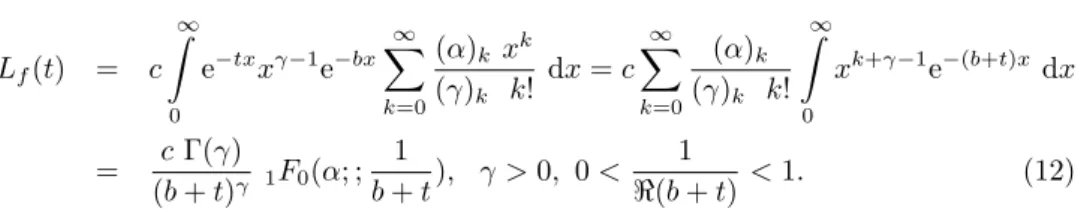
2.2. Laplace Transform
The Laplace transform of f (x), with parameter t, is defined as
Lf(t) =
∞
∫
0
e−txf (x) dx, (11)
whenever the integral is convergent. Then for (4),
Lf(t) = c ∞ ∫ 0 e−txxγ−1e−bx ∞ ∑ k=0 (α)k xk (γ)k k! dx = c ∞ ∑ k=0 (α)k (γ)k k! ∞ ∫ 0 xk+γ−1e−(b+t)x dx = c Γ(γ) (b + t)γ 1F0(α; ; 1 b + t), γ > 0, 0 < 1 ℜ(b + t) < 1. (12)
The moment generating function M (t) of (4) is available from (12) by replacing t by−t and the characteristic function Φ(t) of (4) is available from (12) by replacing
t by−it, where i =√−1.
2.3. Behaviour of the density function
The graph given below shows the general behaviour of the confluent gamma density given in (4), excluding the normalizing constant c. We have drawn the graph for fixed values of γ and b and for varying values of α.
Figure 1 The graph of the density function for γ=2, b=3, and for various values of α
3. Interevent distribution model
In this section, initially we discuss the occurrence of tsunamis due to earthquakes and then investigate the interevent times distribution type.
3.1. Tsunamis due to tectonic earthquakes
Tectonic earthquakes are a particular kind of earthquakes that are associated with the earth’s crustal deformation. Earthquake-induced movement of the ocean floor most often generates tsunamis. When these earthquakes occur under the sea, the water level above the deformed area is displaced from its equilibrium position. Waves are formed as the displaced water mass, which acts under the influence of gravity, attempts to regain its equilibrium. When large areas of the sea floor ele-vate or subside, a tsunami can be created. The pictures shown in this subsection are taken from the site www.enchantedlearning.com
Figure 2 The picture illustrating the occurrence of tsunami due to tectonic earthquakes
Tsunamis are unlike wind-generated waves. The wind-generated waves might have a period of about 10 seconds and a wave length of 150 m. A tsunami, on the other hand, can have a wavelength in excess of 100 km and period on the order of one hour.
Figure 3 The picture showing the intensity of tsunami waves compared to wind generated waves
Tsunamis have a small amplitude offshore and a very long wavelength which is why they generally pass unnoticed at sea, forming only a slight swell above the normal sea surface. They grow in height when they reach shallower water.
Figure 4 The picture showing the characteristics of tsunami waves
A tsunami can occur in any tidal state and even at low tide can still inundate coastal areas. Tsunamis cause damage by two mechanisms: the smashing force of a wall of water travelling at high speed, and the destructive power of a large volume of water draining off the land and carrying a large amount of debris with it, even with waves that do not look large.
3.2. Interevent times
As discussed above, tsunamigenic earthquakes are very powerful and danger-ous and as a consequence, a detailed study on the topics related to earthquakes, tsunamis and their seismicities became essential. Many researchers are engaged in these studies and among them the phenomenon of interevent modelling becomes a main area of study for the last many years. From the recent analysis, it can be seen that the distribution of interevent times and earthquake numbers, as evi-denced by global and regional catalogues exhibit non Poissonian behaviour. Kagan (2010) explains that the earthquake numbers are best fit by a negative binomial distribution, if the magnitude range of the events is large. But, if a restricted magnitude range is selected, then the earthquake numbers including clusters, can be modelled by a Poisson distribution. The tsunami database can be taken as a compilation of different catalogues of tsunami events, tide-gauge reports and individual reports. Moreover, tsunami catalogues include eyewitness observations and post-event tsunami surveys. Data used to analyze tsunami interevent times are obtained from National Geophysical Data Center. The National Geophysical Data Center (NGDC), located in Boulder, Colorado, is a part of the US De-partment of Commerce (USDOC), National Oceanic Atmospheric Administration (NOAA), National Environmental Satellite, Data and Information Service (NES-DIS). NGDC’s mission is to provide long-term scientific data stewardship for the nation’s geophysical data, describing the solid earth, marine, and solar-terrestrial environment as well as earth observations from space, ensuring quality, integrity and accessibility.
A study on the distribution of interevent times, conducted by Geist and Parsons (2008) concludes that there occurs many short interevent times than expected from an exponential distribution associated with a stationary Poisson process. Different statistical models are consistent with the data including the generalized gamma distribution, theoretical distribution derived from ETAS model, inverse Gaussian distribution, Rayleigh distribution etc, see for details Corral (2004), Saichev and Sornette (2007). Let us consider the model given in (4). We compared our model with gamma-Bessel, gamma-Mittag-Leffler and Rayleigh densities. For the anal-ysis, we find the explicit forms of the estimators of the parameters in the density functions using the method of moments. For the whole analysis, Mathematical softwares MAPLE, MATLAB and MATHEMATICA are used.
The method of moments includes the process of equating the sample and popu-lation moments and solving it for the unknown parameters. Inferential procedure of gamma-Mittag-Leffler, gamma-Bessel and Rayleigh models are already
avail-able in the literature. For more details, see Nair (2012) for gamma-Mittag-Leffler model, Sebastian (2012) for gamma-Bessel and Mahdi and Cenac (2006) for Rayleigh model. There, gamma-Mittag-Leffler model with 4 parameters a, α, β, δ is used. The density function is of the form
f (x) = c xβ−1e−axEα,β(−δxα), ℜ(β) > 0, ℜ(α) > 0, a > 0, x > 0,
where Eα,β(−δxα) is the generalized Mittag- Leffler function. The estimators of
parameters are obtained as ˆ β = ∑ (xi− ¯x)3− [ ∑ (xi− ¯x)2][ ∑ x2 i + n¯x] + 2n¯x[n¯x3− ¯x2] ∑ x2 i[4n¯x− 3n − 3] + n¯x2[8n¯x + 13n] + n2x¯ ˆ α = ∑ (xi− ¯x)2− n(¯x − ˆβ)2− n¯x − ˆβ n(¯x− ˆβ) ˆ δ = (¯x− ˆβ) ˆ α + 3¯x− ˆβ. and ˆ a = (2¯x− ˆβ − ˆα) ¯ x + ˆδ .
The gamma- Bessel model considered here, has the form
f (x) = c xβ−1e−ax0F1(; β; δx); x > 0, ℜ(β) > 0, a > 0.
We get the moment estimators as ˆ δ = ∑ (xi− ¯x)2 n − ¯x ˆ β = 2¯x− ∑ (xi− ¯x)2 n− ˆδ . and ˆ a = ∑ (xi− ¯x)3− n¯x ˆ δ + ˆβ .
The Rayleigh model considered here, has the form
f (x) =(x− β) δ2 e
−(x−β)22δ2 , β≤ x < ∞, δ > 0.
The moment estimators are given by
ˆ δ = √ n∑x2 i − ( ∑ xi)2 2n2(1−π 4) and ˆ β = ¯x− ˆδ √ π 2.
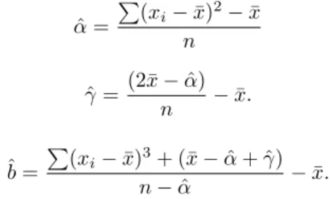
In our model, we get the moment estimators of parameters as ˆ α = ∑ (xi− ¯x)2− ¯x n ˆ γ = (2¯x− ˆα) n − ¯x. and ˆ b = ∑ (xi− ¯x)3+ (¯x− ˆα + ˆγ) n− ˆα − ¯x.
Now we consider the histogram of the data embedded with gamma-Bessel, gamma-Mittag-Leffler, Rayleigh and our new probability models. Here the x- axis values denote the number of days. The same program generated the four different graphs as shown below.
Figure 5 The graph of histogram embedded with the probability models
We calculated Pearson’s χ2 statistic with 10 degrees of freedom for the four different probability models. For Rayleigh density, the value of the statistic is obtained as 16.44. For the gamma-Bessel model, the value of the statistic is 17.12. For the gamma-Mittag-Leffler model, the value is 12.71 and for our new probabil-ity model, the value is 8.07. From the table, the value obtained is 18.307. We can see that the four different probability models are consistent with the data. But the distance measure of the statistic of our new probability model is less than that of the other three probability models and from the graphs generated by the same program, we can conclude that our model better fits the data than the other three.
ACKNOWLEDGEMENTS
The author would like to thank the Department of Science and Technology, Government of India, New Delhi, for the financial assistance for this work un-der project-number SR/S4/MS:287/05, and the Centre for Mathematical Sciences for providing all facilities. The author acknowledges gratefully the guidance and encouragement of Professor A.M.Mathai, Director of the Centre for Mathematical
Sciences, in this research work. The author also acknowledges the support of Dr. Umesh Singh, Professor of Statistics, Banaras Hindu University, Varanasi, India, in this research work.
REFERENCES
J. Aitchison, J.A.C. Brown (1957), The lognormal distribution with special
reference to its uses in economics, Cambridge University Press.
H.K. Cigizoglu, M. Bayazit (2000), A generalized seasonal model for flow
duration curve, Hydrological Processes, 14, pp. 1053-1067.
R.E. Collin (1960), Field Theory of Guided Waves, Mc-Graw-Hill, New York. A. Corral (2004), Universal local versus unified global scaling laws in the
statis-tics of seismicity, Physica A 340, pp. 590-597.
L.B. Felsen, N. Marcuvitz (1973), Radiation and Scattering of Waves, vol. 1, Englewood Cliffs: Prentice-Hall, NJ.
E.L. Geist, T. Parsons (2008), Distribution of tsunami interevent times, Geo-physical Research Letters 35, L02612. doi: 10.1029/2007GL032690.
A.K. Gupta, S. Nadarajah (2006), Sums and ratios for beta Stacy distribution, Applied Mathematics and Computation 173, pp. 1310-1322.
O.A.Y. Jackson (1969), Fitting a gamma or log-normal distribution to
fibre-diameter measurements on wool tops, Applied Statistics 18, pp. 70-75.
Y.Y. Kagan (2010), Statistical distributions of earthquake numbers: consequence
of branching process, Geophysical Journal International 180, pp. 1313-1328.
H.A. Lauwerier (1951), The use of confluent hypergeometric functions in
math-ematical physics and the solution of an eigenvalue problem, Applied Scientific
Research 2, pp. 184-204.
E. Lukacs (1955), A characterization of the Gamma distribution, The Annals of Mathematical Statistics 26(2), pp. 319-324.
S. Mahdi, M. Cenac (2006), Estimating and Assessing the Parameters of the
Lo-gistic and Rayleigh Distributions from Three Methods of Estimation, (Caribbean
Journal of Mathematical and Computing Sciences) 13, pp. 25-34.
A.M. Mathai (1993), A Handbook of Generalized Special Functions for Statistical
and Physical Sciences, Clarendon Press, Oxford.
A.M. Mathai (2005), A pathway to matrix - variate gamma and normal densities, Linear Algebra and its Applications 396, pp. 317-328.
A.M. Mathai, H.J. Haubold (2008), Special Functions for Applied Scientists, Springer, New York.
A.M. Mathai, P.N. Rathie (1971), Exact distribution of Wilks’ criterion, The Annals of Mathematical Statistics 42, pp. 1010-1019.
S.S. Nair (2012), Statistical Distributions Connected with Pathway Model and
Generalized Fractional Integral Operator, Dissertation, pp. 35-54.
S.B. Provost (1986), The Exact Distribution of the Ratio of a Linear
Combina-tion of Chi-Square Variables over the Root of a Product of Chi-Square Variables,
The Canadian Journal of Statistics 14, pp. 61-67.
A. Saichev, D. Sornette (2007), Theory of earthquake recurrence times, Jour-nal of Geophysical Research 112. doi:10.1029/2006JB004536.
N. Sebastian (2011), A generalized gamma model associated with a Bessel
func-tion, Integral Transforms and Special Functions 22(9), pp. 631-645.
N. Sebastian (2012), Statistical Distributions And Time Series Models Connected
To Bessel And Mittag-Leffler Functions Via Fractional Calculus, Dissertation,
pp. 43-60.
M.K. Simon, M.S. Alouini (2004), Digital Communication over Fading
Chan-nels, 2nd edition, Wiley, New York.
L.J. Slater (1960), Confluent Hypergeometric Functions, Cambridge University Press.
N.M. Thomas (2011), Distribution of products of independently distributed
path-way random variables, Statistics: A Journal of Theoretical and Applied
Statis-tics, 47(4), pp. 861-875.
SUMMARY
Confluent gamma density in modelling tsunami interevent times.
We consider here a probability model which associates the usual gamma form with a confluent hypergeometric series. The probability model is termed as confluent gamma density. Some distributional properties of this model are derived. A graphical represen-tation of the model for the varying values of parameter is illustrated. The model thrusts into an interesting application which relates it with tsunami event modelling. A study on tsunami occurrence is essential since it happens frequently at different parts of the world. Here we give an overall view about tsunamis and analyze tsunami interevent times. Keywords: gamma model; confluent hypergeometric series; G-function; tsunami events