Estad´ıstica
A comparative analysis of tree-based models
classifying imbalanced breath alcohol data
Manuela Alca˜niz and Miguel Santolino Department of Econometrics University of Barcelona [email protected], B [email protected] Llu´ıs Ramon Data Scientist Digital Origin [email protected] Abstract
When applied to binary data, most classification algorithms behave well provided the dataset is balanced. However, when one single class includes the majority of cases, a good predictive performance for the minority class is not easy to achieve. We examine the strengths and weaknesses of three tree-based models when dealing with imbalanced data. We also explore sampling and cost sensitive methods as strategies for improving machine learning algorithms. An application to a large dataset of breath alcohol content tests performed in Catalonia (Spain) to detect drunk drivers is shown. The Random Forest method proved to be the model of choice if a high performance is required, while down-sampling
strategies resulted in a significant reduction in computing time. When predicting alcohol impairment, the area of control (built-up or not), hour of day and driver’s age were the most relevant variables for classification.
Keywords: Imbalanced data, positive, drunk driving, police, checkpoint, machine learning.
1. Introduction
Tree-based models have attracted the increasing attention of researchers in recent years; however, analyses of the use of such models when there is a highly unequal distribution between classes are scarce. This is particularly true of binary data where one class includes the majority of cases and the other represents just a small portion. Imbalanced datasets of this kind are very common in such disciplines as medical diagnosis, on-line advertising, fraud detection, network intrusion, road safety, etc.
Many classification algorithms behave well for balanced datasets; yet, when applied to imbalanced data, model fitting may be biased towards the majority class. As a result, the model may provide a poor predictive performance for the minority class, which is usually the most interesting one. Kumar and Sheshadri [20], He and Garcia [16] and Chawla [9] review problems of class imbalance and alternative solutions. Here, the performance of two strategies for dealing with imbalanced data –that is, sampling and cost sensitive methods– are compared, and the interpretability of their respective results is discussed.
Specifically, we illustrate the performance and features of tree-based models by applying them to the classification of alcohol-impaired drivers in Catalonia (Spain). When testing for breath alcohol content (BrAC) over the legal limits, highly imbalanced results are obtained –clearly, most drivers are not
alcohol-impaired and so BrAC tests are largely negative.
The identification and deterrence of potential alcohol-impaired drivers is a priority for traffic authorities the world over ([24]) and while a downward trend in drunk driving has been observed in many countries, there is still room for improvement ([32], [24], [34]). For example, in 2014, 24.8% of deaths among drivers in Catalonia were related to alcohol. In order to tackle drunk driving effectively, appropriate policies need to be adopted. In this paper three tree-based models are studied and their application to the classification of drivers with a BrAC over the legal limit on Catalan roads is explored. Specifically, we examine the use of the Classification and Regression Tree, Tree Bagging and the Random Forest models to classify positive BrAC tests.
Several studies have been conducted in Catalonia with regard to drinking habits and driving. Alca˜niz et al. [1] estimated the prevalence of alcohol-impaired driving in Catalonia in 2012. They found that it was the 1.29% for the general population of drivers, 1.90% on Saturdays and 4.29% on Sundays. Chulia, Guillen, and Llatje [10] studied seasonal and time-trend variation by gender of alcohol-impaired drivers at preventive sobriety checkpoints. Alca˜niz, Santolino, and Ramon ([2], [3]) studied age-drinking patterns and drinking behavior in Catalonia and analyzed different strategies in sobriety checkpoints. They suggested that non-random breath tests were primarily effective to detect binge drinking and random breath tests in detection of other drinking and driving profiles of population. To our knowledge, classification models to identify drunk drivers have not been previously applied to Catalan road data.
The rest of this paper is structured as follows. Following on from this introduction, in Section 2, three tree-based models are introduced along with their properties and variants, and various approaches to tackling the class imbalance problem are described.
Section 3 is devoted to explaining the dataset obtained from police preventive checkpoints. The results obtained after fitting the tree-based models to the data and several variants are reported in Section 4. Concluding remarks and discussion are outlined in Section 5.
2. Methods
In this section three tree-based models are introduced and their properties discussed. Specifically, we analyze the Classification and Regression Tree, the Tree Bagging and the Random Forest models1.
A number of extensions employing other types of response data and alternative implementations are also detailed. Finally, we investigate how to deal with the class imbalance problem.
2.1. Classification and Regression Trees
Classification and Regression Trees (CART) were first introduced by Breiman et al. [8]. The CART model partitions the predictor space in a recursive way so as to create groups in the response variable that are as homogeneous as possible. The CART algorithm begins by splitting the dataset into two disjoint subsets (known as nodes or leaves). For each predictor, splits are computed for all possible cut-off values and the one that maximizes the homogeneity (and minimizes the impurity) of the resulting disjoint subsets is chosen. This process is recursively repeated for each node.
An impurity measure, quite commonly the Gini index, is used to choose the best split, with the split impurity being calculated by aggregating the impurity of the subnodes. For a two-class problem, the Gini index for a given node is defined as p1(1 − p1) + p2(1 − p2),
where p1and p2are the class 1 and class 2 probabilities, respectively
1
The CART and Random Forest trademarks are licensed exclusively to Salford Systems.
[19]. Alternative measures to the Gini index exist. For instance, the information gain measure can be used, although differences are frequently not significant [27]. To avoid the overfitting of the CART model, the subtree is selected based on a cost complexity tuning, where a complexity parameter cp penalizes the size of
the tree. In fact, the subtree that minimizes Impuritysubtree +
cp × (Number Terminal Nodes) is selected. The cp value, the
hyperparameter, is normally selected using cross-validation (CV). CART models have the advantage of being easy to interpret and rapid to compute, of allowing missing values to be dealt with and of facilitating feature selection. An important characteristic of these models is that variable importance can be assessed. This is achieved by retaining the reduction in the Gini index at each split and aggregating these values for every predictor. Predictors that either appear at the beginning of the tree or which are used in several splits are more important. Note that variable importance can be biased when there are many missing values or there are categorical variables with many levels ([30], [21]). The main disadvantages of CART models concern the instability of their results.
In practice, a large number of alternative implementations of tree models exist. Different approaches have been proposed for their use with survival data [5], multivariate regression [11], clustering [29] and unbiased models ([17], [21]). Hyafil and Rivest [18] show that constructing optimal binary decision trees is an infeasible task. Grubinger, Zeileis, and Pfeiffer [14] propose evolutionary algorithms to improve accuracy, while Loh [22] compares a set of alternative implementations in terms of their capabilities, strengths, and weaknesses.
2.2. Tree Bagging
Bagging, or Bootstrap aggregating, also introduced by Breiman [6], involves generating several predictions and combining them to
obtain an aggregated predictor. Here, predictions are generated by applying a model to different bootstrap replicas of the dataset. These replicas are made by replacement and are as large as the dataset itself. The aggregate is the majority vote of all models. Each tree used in the tree bagging is computed as described in 2.1 above. The only difference is that there is no pruning step. The aggregating step neutralizes the overfitting error of the trees.
The number of trees to be used is defined by the user and, in practice, a small number of replicas usually proves sufficient [19]. Although the error decreases with the number of trees, the trees are highly correlated, so the margin of improvement associated with each additional tree decreases with the number of replicas. Compared with CART models, the advantage of tree-bagging models is their stability, which reduces the risk of overfitting. On the other hand, these models are computationally more intensive than CART models and their interpretation more complex.
2.3. Random Forest
In common with the two models outlined above, the Random Forest (RF) model was proposed by Breiman [7]. RF involves generating bootstrap replicas of the original dataset and creating trees for each replica as in Bagging. However, RF seeks to create uncorrelated trees to improve predictions. To create trees that are as different as possible, at each split the trees can only use a limited number of random variables. Hence, the trees tend to be very different and provide different information when aggregated.
As in Tree Bagging, the number of trees to compute has first to be specified. The number of variables that might be split at each node (referred to as mtry) must also be defined. A common selection is the square root of the number of variables [19]. In common with the previous models, the minimum number of nodes can also be determined. The higher this number is, the smaller and faster the
trees will be. As with the Tree Bagging models, the advantages of RF models is that performance is enhanced and the overfitting risk reduced. Furthermore, RF models are robust to outliers. Their disadvantages include the complexity of interpretation and the lengthy computation time.
Indeed, the computation time of the original RF can be prohibitive in the case of a large mtry and/or a high number of trees. Therefore, less timing-consuming, more intensive alternatives are useful. Here, we use an efficient RF implementation as ranger2. An
additional feature of ranger is that it uses a variant for probability estimation. Each tree provides the proportion of positives as opposed to its classification. The probability is obtained by averaging this proportion for all the trees. In doing so, the model performance is generally improved [23].
Sometimes categorical variables can be interpreted as ordered categorical variables (for instance, colors ordered according to their intensity or type of roads based on their traffic capacity). This strategy can significantly reduce the computation time of RF. To split a categorical variable of n categories, the algorithm checks all 2(n−1)− 1 possible combinations. However, since the categories are
sorted in the case of ordered categorical variables, the impurity is calculated between each category, and the threshold that gives the best split is chosen. This is much quicker to compute as only one variable has to be checked.
RF models can assess variable importance in three ways. The simplest way is to count the number of times that a variable is selected in all the trees. The second way involves computing the aggregate reduction in impurity obtained at each split in all the trees. Finally, a third way is to measure the permutation importance. For
2
This reduced computing time by a factor of 12 compared to that of the original RF.
each tree, the prediction performance of out-of-bag (OOB) samples3
is recorded. This performance is again computed but here using the values of one randomly permuted variable. The drop in performance resulting from this permutation is averaged over all the trees. This is carried out for each variable and provides a measure of variable importance in the RF [[15]. When variables are highly correlated or if categorical and continuous variables are combined, the variable importance indicator needs to be considered with caution[31].
RF models have been extensively applied. For instance, generalizations of RF models have been proposed to provide conditional quantiles and confidence intervals ([25], [33]). Segal [28] demonstrates that RF can overfit datasets with large numbers of noisy inputs. To deal with this, alternative extended RFs have been proposed ([35], [4]).
2.4. Class Imbalance
It is relatively common to find imbalanced datasets, where the majority of cases present negative outcomes. For example, only a small percentage of observations show positive outcomes in datasets of BrAC tests. Many classification algorithms have been designed specifically for balanced datasets and so a poor predictive performance may be obtained when applied to imbalanced data. Two strategies for dealing with unbalanced data are sampling methods and cost sensitive methods.
Sampling methods involve modifying the original dataset to obtain a balanced dataset and they can be divided into the following categories: down-sampling, i.e., excluding some instances of the majority class by random sampling; up-sampling, i.e., incorporating more instances of the minority class by random sampling with
3
Out-of-bag samples consist of observations not included in a bootstrap sample.
replacement; and, hybrid methods, i.e., combining both up- and down-sampling methods. Note that sampling methods apply only to training data and not to testing data. Cost-sensitive methods involve applying different costs of misclassification to each class in the model fitting process. By specifying a higher cost to the misclassification of a minority instance than that to a majority instance, the machine learning algorithm makes fewer errors with the minority class, as it is more expensive. This would counteract the bias towards the majority class.
An additional problem presented by class imbalance is how best to assess classifiers. The usual classification metric is the level of accuracy, for instance, by means of confusion matrix. However, in the case of imbalanced data, this measure may be inadequate. Other techniques to compare tree-based models such as leave-one-out cross-validation can be in addition computationally very expensive for large datasets. To overcome these limitations, receiver operating characteristic (ROC) curves are used. The ROC curve presents a binary classifier performance when its threshold varies. It is formed by plotting the true positive rate (TPR) against the false positive rate (FPR) at various threshold settings. Any point on the diagonal of the ROC curve is a random guess classifier, while any points below the diagonal are worse than a random guess. A complete description of ROC analysis can be found in Fawcett [12].
To compare the performance of different classifiers directly, we use the area under the ROC Curve (AUC). This indicator aggregates all the information provided by the ROC curve in a single scalar expression. A classifier with a high AUC indicates that it has a better than average performance. Note, however, that the first classifier may present a worse performance than the second classifier in a specific region of the ROC curve. An interesting property is that the AUC of a classifier is equivalent to the probability that the
classifier will rank a randomly chosen positive instance higher than a randomly chosen negative instance [12].
3. Data
3.1. Drunk driving legislation
Statutory blood-alcohol limits for driving differ across the countries of Europe. Spanish legislation differentiates between administrative and criminal positives, according to the level of alcohol concentration in the breath (or blood). Drivers with BrAC levels between 0.25 and 0.60 mg/l (0.15 and 0.60 mg/l for novice and professional drivers) face administrative penalties if detected. When the BrAC level is over 0.60 mg/l, drivers are deemed to have committed a criminal offence and, therefore, face more stringent legal sanctions, including temporary suspension of the driving license and imprisonment.
The police are allowed to perform a BrAC test on any driver, even if the driver does not show any symptoms of alcohol impairment. The standard procedure is to conduct a BrAC test using a portable breathalyzer while the driver is seated in their car. If negative, the driver is allowed to continue on their journey; if positive, given that the breathalyzer has no legal validity, an evidential breath test is performed in the officer’s vehicle.
3.2. Variables
The database comprises 439,699 preventive BrAC tests carried out at checkpoints by traffic authorities in 2014 in Catalonia. These tests represent almost 95% of the total number of BrAC tests, while the remaining 5% includes tests conducted on drivers showing visible signs of alcohol intoxication or after committing a traffic violation or on drivers involved in a traffic accident. Preventive BrAC tests performed on cyclists or pedestrians were removed from
the database. Observations with missing information were also removed. The final database comprises 408,936 BrAC tests.
Information recorded by traffic officers, including the location of the checkpoint, specific hour of day, driver characteristics and vehicle type, is available. Information about location differentiates between interurban and urban areas and records the region and subregion in which the checkpoint was set up. The territory of Catalonia is divided into four administrative units and is recorded here as the variable region. However, there is a more detailed administrative division composed of 41 subregions. The traffic police in Catalonia include both the regional police (Mossos d’Esquadra) and the local police. There is a traffic police administrative division, known as ART, which comprises eight levels and corresponds to the scale between that of the regions and subregions.
The variable roadType records the type of road on which the BrAC test was performed4. Information about the hour, day, week
and month when the test was performed is also available. As drinking habits are closely associated with leisure, factors identifying bank holidays (holiday), the eve of such holidays (holidayEve) and long weekends (longWeekend ) were created. Finally, driver and vehicle characteristics were also recorded.
The description of variables is as follows.
❼ positive (Dependent variable): BrAC level above legal limit (yes/no).
❼ builtUp: Interurban area or Urban area.
❼ region: Barcelona, Girona, Lleida and Tarragona. ❼ subregion: Name of subregion, 41 categories. 4
Highway1 corresponds to toll-highways and Highway2 corresponds to toll-free highways.
❼ policeType: Regional police or Local police. ❼ ART : Police territorial division, eight categories.
❼ roadType: Highway1, Highway2, Conventional road, Rural road and Urban road.
❼ hour: specific hour of day (number 1-24) when the BrAC was performed.
❼ day: day when the BrAC was performed. ❼ month: month when the BrAC was performed.
❼ week: week when the BrAC was performed, as a number (1-52).
❼ weekday: day of the week when the BrAC was performed, as a number (1-7, Sunday being 7).
❼ dayType: Mon-Thu, Fri, Sat and Sun.
❼ workingDay: 1 if it was a working day, 0 otherwise.
❼ timePeriod: morning (6:00 to 13:59), afternoon (14:00 to 21:59) or night (22:00 to 5:59h).
❼ holiday: bank holiday (yes/no).
❼ holidayEve: Eve of bank holiday (yes/no) ❼ longWeekend: Long weekend (yes/no) ❼ sex: driver’s sex.
❼ age: driver’s age.
❼ spanish: driver Spanish or foreigner.
❼ vehType: type of vehicle (Car, Van, Motorcycle, Moped, Light truck, Heavy truck, Bus, and Other).
Algorithms of tree-based models implement an implicit variable selection, so the strategy involved including all the variables in the models. Table 1 presents the number of tests, number of positives and the percentage of positives for the main variables and their levels. Additional tables for variables comprising many levels are included in the appendix: ART (Table A.1), month (Table A.2) and hour of day (Table A.3), are included.
3.3. BrAC outcomes above legal limit
The positive response variable is highly skewed. Of the 408, 936 BrAC tests carried out, only 16, 494 –approximately 4% –were positive. Figure 1 shows the percentage of BrAC tests above the legal limit by subregion. The map shows a non-homogeneous percentage of positives throughout the territory, with values being particularly high in the north-east and along the coast.
Figure 2 shows the percentage of BrAC tests above the legal limit according to a specific set of variables. In winter there are fewer positives, while from June to September there is a greater number. Urban areas are associated with a higher prevalence of positives than are interurban areas. During the week there is a 2% positive rate, while on weekends it is between 5 and 7%. Positive rates on Fridays (3.5%) are halfway between weekday and weekend prevalences. A similar percentage of positives is observed for both men and women; however, non-Spanish men record a slightly higher positive rate, while non-Spanish women present the lowest rate. Driver age is also informative. The prevalence of alcohol peaks at age 20 with more than 7% of positives and falls after that age. The final plot analyzes the relationship between the prevalence of alcohol with the hour of
Variable Levels # tests # positives (%) builtUp Interurban area 267,117 10,149 3.8
Urban area 141,819 6,345 4.5
region Barcelona 225,019 9,944 4.4
Girona 50,145 2,610 5.2
Lleida 61,868 1,020 1.6
Tarragona 71,904 2,920 4.1
policeType Regional police 266,029 10,155 3.8 Local police 142,907 6,339 4.4 roadType Highway1 30,149 1,213 4.0 Highway2 45,735 2,247 4.9 Conventional road 190,744 6,674 3.5 Rural road 489 15 3.1 Urban road 141,819 6,345 4.5 dayType Mon-Thu 180,635 4,007 2.2 Fri 58,093 2,089 3.6 Sat 85,250 4,637 5.4 Sun 84,958 5,761 6.8
workingDay Working day 206,126 5,277 2.6 Non-working day 202,810 11,217 5.5 timePeriod Morning 101,590 3,576 3.5 Afternoon 86,982 985 1.1 Night 220,364 11,933 5.4 sex Man 332,411 13,430 4.0 Woman 76,525 3,064 4.0 age3l [15,30] 133,713 7,732 5.8 (30,45] 171,145 6,023 3.5 (45,100] 104,078 2,739 2.6 licenseYear [1932,1994) 138,129 3,964 2.9 [1994,2004) 115,267 4,154 3.6 [2004,2012) 131,088 7,043 5.4 [2012,2015) 24,452 1,333 5.5 spanish Spanish 350,444 14,035 4.0 Non-Spanish 58,492 2,459 4.2 vehType Car 316,530 14,332 4.5 Van 25,229 436 1.7 Motorcycle 29,717 1,264 4.3 Moped 8,876 334 3.8 Light Truck 6,117 25 0.4 Heavy Truck 19,361 78 0.4 Bus 2,490 12 0.5 Other 616 13 2.1
Table 1: Number of tests, positives and percentage of positives for main variables.
Figure 1: Percentage of positives by subregion.
the day and the driver’s age. This highlights a black spot in the early morning for drivers in the young age group when 15% of BrAC positives are recorded. All age groups present a high positive rate between 9pm and 3am. In the afternoon, this percentage increases with age. Finally, a black spot occurs at 13h in the 55 to 65 age group.
4. Results
To assess the performance of the tree-based models, the data were randomly split into training and test sets. The division was made preserving the distribution of positives-negatives and of the
other variables. The training set contained 70% of the data and was used to fit the models; the test set contained the remaining 30% of the data and was used to validate the models. All categorical variables were included in the models as binary variables; that is, each category was converted into a dichotomous variable. The performance of all the models was based on the AUC from the test set. All models were performed with R version 3.2.3 [26]. Packages used were caret, randomForest, ranger, pROC, e1071, rpart, ipred, plyr and dplyr.
When a hyperparameter had to be adjusted, a ten-fold cross-validation (10-CV) was used; that is, the training dataset was randomly split into ten partitions. The model/hyperparameter was trained with nine of the ten original partitions. The remaining partition was used to obtain the validation performance of the model. This step was repeated ten times and a different partition was used each time for validation. The model/hyperparameter performance was thus obtained as an average of all the validations. The metric for hyperparameter tuning was the AUC value. The hyperparameter with the highest AUC was selected5. Once the hyperparameter was
adjusted, the model was fitted to the whole dataset.
4.1. Classification and Regression Tree model
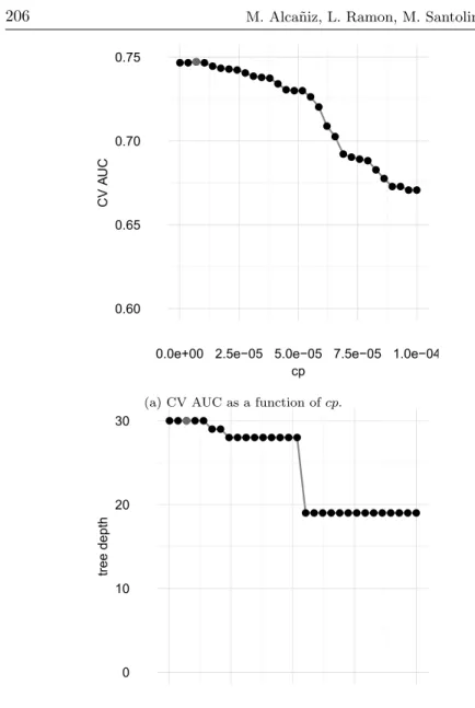
Tree models contain an hyperparameter which is the complexity parameter (cp). A grid of 50 (cp) values was used. The best cross-validated cp value was 6.9897 · 10−6, with an AUC of 0.7472.
First panel of Figure 3 shows that the AUC value increases when the cp decreases.
Note that the adjusted cross-validated cp value was very small. 5
Alternatives exist for selecting the tuning parameters, such as the one standard error rule or tolerance. These alternatives choose the simplest model within a standard error or a defined tolerance from the best model, respectively [16].
0.60 0.65 0.70 0.75
0.0e+00 2.5e−05 5.0e−05 7.5e−05 1.0e−04 cp
CV
A
UC
(a) CV AUC as a function of cp.
0 10 20 30
0.0e+00 2.5e−05 5.0e−05 7.5e−05 1.0e−04 cp
tree depth
(b) Tree depth as a function of cp.
Figure 3: CART models. Model with the best AUC is shown in red. Left panel: CV AUC as a function of cp. Right panel: Tree depth as a function of cp.
The fitted trees need to be very deep in order to appreciate differences between the two classes. Right panel of Figure 3 shows the tree depth as a function of cp. Note that the highest AUC was obtained in the trees with 30 levels. The interpretation of deep trees is more complex. Using the adjusted cp value, a final model was adjusted with all the training data. A membership probability was obtained from the test set. The test AUC value was 0.7498.
These previous models do not take into account the fact that the data are imbalanced. Therefore, two approaches for dealing with imbalanced data were applied. First, down-sampling was performed and so the training data were reduced to a down-sampled training dataset. This contained the same number of observations from each class. Our results improved in comparison to our previous outcomes. The best cross-validated cp value was 4.9310 · 10−4, with an AUC of
0.7499. Note that this cp value is 50 times higher than the previous cp. The fitted tree has a depth of 17 levels and the AUC associated with the test set was 0.7577. Thus, using a subset of the dataset resulted in a better performance.
Second, up-sampling was performed. To achieve a balanced dataset, items from the minority class were added until the dataset contained the same number of positives as negatives. A large overfit was made in cross validation. To obtain a balanced dataset, many instances from the minority class had to be copied. For this reason, the fitted tree contained the same observations in the leaves as in the validation set. This resulted in nearly perfect performance, but when tested with new data, a very poor performance was obtained. Although the cross-validated AUC value was almost 1, when the model was validated with the test data, its AUC was less than 0.5, i.e., a random guess.
Finally, a cost sensitive method was applied. The selection of the cost value had first to be defined. We used cost values that balanced
the difference between classes. The dataset contains one positive for every 20 negatives; thus, the tree model performance was analyzed by applying a cost of 10, 20 and 30 for misclassification. Table 2 shows the cp value, the cross-validated AUC, the test AUC and the depth for each cost value.
Cost Best cp CV AUC test AUC tree depth
10 0.000277 0.7483 0.7570 21
20 0.000311 0.7560 0.7663 17
30 0.000242 0.7545 0.7630 28
Table 2: Model results by the cost used.
The best model performance was obtained when a misclassification cost of 20 was applied. Compared to the base tree, the cp values were much higher and the trees were less complex. Yet, they were still too deep to be visually interpretable. If an interpretative tree is desired for our context, a bigger cp value needs to be chosen as a trade-off between interpretability and predictive performance.
4.2. Tree Bagging model
Bagging consists of generating several bootstrap replicas from the original dataset and modeling the deepest possible tree for each replica. Whereas bagging has no hyperparameters to tune, the number of bootstrap replicas does have to be defined. In our case, the number of bagging trees was 50 and the test AUC was 0.7267. Figure 4 (a) shows that increasing the number of replicas did not improve the test AUC. Note that after 40 replicas, the performance of the model increases very slowly. When a sufficiently high number of trees had been used, adding another tree did not provide any additional information, since it was highly correlated with some other previous tree.
Class imbalance strongly affected bagging performance. To predict a new observation, class predictions were obtained for each tree and the predicted probability was obtained from the frequency of all individual tree predictions. This can be explained by the fact that each tree in the bagging provides a classification, not a probability. For example, a leaf with five negatives and four positives would be classified as negative, just as would a leaf with all negatives. As in the case of the tree model, a sampling approach was adopted. Here, only the down-sampling method was used. Bagging was applied with 50 trees and a test AUC of 0.7675 was obtained. Finally, a cost sensitive approach was performed. A cost of 20 was applied to the bagging building step and a test AUC value of 0.7737 was obtained. Note that using different costs affects how the splits are chosen in the tree building step. As bagging builds trees that are as deep as possible, the final leaves tend to be more homogeneous so as to avoid misclassification costs. This limitation does not occur in the base bagging model. Figure 4 (b) shows the ROC curve of the base Tree Bagging model and the down-sampling and cost sensitive Tree Bagging models.
To conclude, we should stress that the Bagging Models were computationally much more intensive than the Classification and Regression Tree models. Indeed, in some cases the model fitting took more than twelve hours.
4.3. Random Forest
The efficient Random Forest implementation ranger was used and categorical variables were considered as ordered categorical variables. Compared to the RF model that does not modify categorical variables, the AUC values were not statistically significantly different6; however, the computation time was halved.
6
The CV AUC of the RF with original categorical variables was 0.7886 (s.d.=0.0065), and the CV AUC of the RF with converted categorical variables
0.65 0.70 0.75 0.80
0 10 20 30 40 50
Number of bootstrap replicas
T
est
A
UC
(a) Test AUC by the number of bootstrap replicas.
0.00 0.25 0.50 0.75 1.00 0.00 0.25 0.50 0.75 1.00
False Positive Rate
T rue P ositiv e Rate base cost down
(b) ROC curves by the bagging models used.
Figure 4: ROC curves and number of bootstrap replicas. Left panel: Test AUC by the number of bootstrap replicas. Right panel: ROC curves by the bagging models used.
Intuitively it seems that performance is markedly affected when considering ordered categorical variables. This might be because some categorical variables are directly considered as ordered (dayType, timePeriod ) or, at least, are categorized with a certain order. For instance, the variable roadType has a certain order, beginning with road types that have higher speed limits and terminating with those with a slower speed limit.
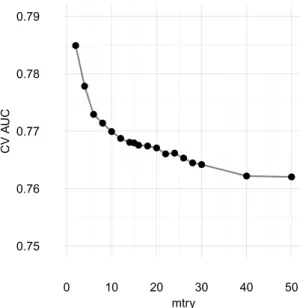
With a ten-fold CV, a large number of different mtry was considered for selection. Figure 5 shows that CV AUC increased as the number of mtry decreased. The highest CV AUC was obtained with an mtry equal to two. It had a CV AUC of 0.7849 and a test AUC of 0.7932. A low mtry means that trees are very different from each other, so each provides information for the aggregation step. A low mtry could be problematic in the case of a high number of non-informative variables, which does seem to be the case here.
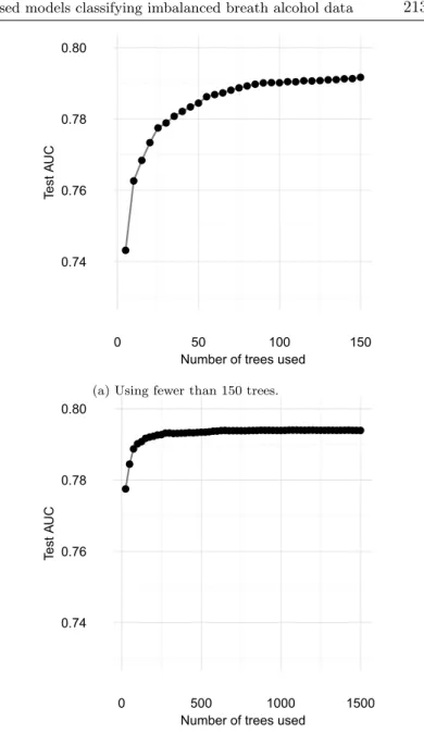
Once the mtry was selected, the number of trees to be used was analyzed. Figure 6 shows model performance as a function of the number of trees. When the forest was small, adding new trees substantially improved the model performance. However, the test AUC value did not increase after approximately 400 trees.
Finally, the down-sampling strategy was adopted to deal with class imbalance problems. The down-sampled performance of the model was slightly worse than when using all the dataset. The optimal mtry was three with an associated CV AUC value of 0.7753 and a test AUC value of 0.7871. Compared with the previous models, the standard deviation was much higher. As each fold used fewer data, the AUC results were more dispersed. In terms of speed, the down-sampled performance was fifteen times faster than when using all the data. The cost sensitive approach was not performed. was 0.7820 (s.d.=0.0064).
0.75 0.76 0.77 0.78 0.79 0 10 20 30 40 50 mtry CV A UC
Figure 5: CV AUC as a function of mtry.
Variable importance
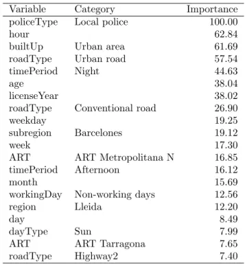
A major advantage of the RF model is that variable importance can be assessed. Here, we evaluate variable importance by means of the RF built-in permutation variable importance measure, which compares the increase in the prediction error after permuting all elements of a variable. Here, categorical variables were not converted to ordered categorical variable but to dummy variables in order to facilitate interpretation.
Table 3 shows the 20 variables with the highest values on the permutation variable importance measure. The variable with the highest value was Local police. The correlated categories of Urban area (builtUp) and Urban road (roadType) were in third and fourth
0.74 0.76 0.78 0.80
0 50 100 150
Number of trees used
T
est
A
UC
(a) Using fewer than 150 trees.
0.74 0.76 0.78 0.80
0 500 1000 1500
Number of trees used
T
est
A
UC
(b) Using fewer than 1500 trees.
Figure 6: Test AUC as a function of the number of trees. Left panel: Using fewer than 150 trees. Right panel: Using fewer than 1500 trees.
positions. This means that the behavior of the Local police and the Regional police was considered to be different by the RF algorithm. As expected, the hour and the time period-night were relevant for the classification of observations. The most important characteristics of the driver profile were age and experience (number of years holding a driver’s license) which are both ranked in the top ten variables by importance. The remaining variables in the top 20 were road type, some regions/subregions and police divisions, and variables related to the weekday and week of the year. Notice that sex and vehicle type do not figure in the top 20.
Variable Category Importance
policeType Local police 100.00
hour 62.84
builtUp Urban area 61.69
roadType Urban road 57.54
timePeriod Night 44.63
age 38.04
licenseYear 38.02
roadType Conventional road 26.90
weekday 19.25
subregion Barcelones 19.12
week 17.30
ART ART Metropolitana N 16.85
timePeriod Afternoon 16.12
month 15.69
workingDay Non-working days 12.56
region Lleida 12.20
day 8.49
dayType Sun 7.99
ART ART Tarragona 7.65
roadType Highway2 7.40
4.4. Comparison of tree-based models
To conclude, summarizing results are shown in Table 4. All the tree-based models discussed in the article are compared in terms of classification performance and computation intensity.
Tree-based Test AUC Time computation
model intensity
CART 0.7498 Low
Down-sampling CART 0.7577 Low Up-sampling CART <0.5 Low/middle Cost sensitive CART 0.7663 Low
Bagging 0.7267 Very High
Down-sampling Bagging 0.7675 High Cost sensitive Bagging 0.7737 Very high Efficient Random Forest 0.7932 Middle/high Down-sampling efficient 0.7871 Middle Random Forest
Table 4: Performance and time consuming comparison of tree-based models.
5. Discussion
This paper compares the use of three tree-based models used in classification problems –in this specific case, as applied to BrAC test results in excess of the legal limit in Catalonia (Spain). Drunk driving data are deeply imbalanced since most drivers are not alcohol impaired. Additionally, the performances of two alternative strategies for dealing with imbalanced data –sampling methods and cost sensitive methods– are compared. Unlike up-sampling, down-sampling methods were preferred to the original methods. The results following the application of down-sampling methods were often slightly worse, but the reduction in computing time was
significant. As such, down-sampling techniques may be used to obtain a rapid overview of model performance. In our case more data did not improve model performance substantially. In the case of imbalanced datasets, quality may be more important than quantity. A comparison of the tree-based methods, showed that the Random Forest model performed best, which means it can be considered the model of choice if a high performance model is wanted. If rapid computation is required, however, the (CART) tree model with misclassification costs should be used. Finally, when compared to these two methods, Tree Bagging offered no modeling advantages in the context described here.
In terms of the number of nodes, trees were in general very deep, hindering the direct interpretation of variables. According to the Random Forest variable importance indicators, the most important variables were those of the area of control, the hour of day and the driver’s age, findings that are in line with previous studies ([1], [13], [3],[2], [10]). Built-up/non-built-up areas was the most important variable in the classification. As for the implications of our findings for road safety, it is clear that different enforcement strategies are required to address drunk driving in each of the two areas. An interesting application of tree-based methods is their utility for helping in-situ police officers select the drivers that should be tested when the checkpoint is set up. This application could be extended to drug testing since the unitary cost of drug tests is high in comparison to that of alcohol tests.
Future areas of research include to distinguish between administrative and criminal offenses. In this highly imbalanced scenario it would be interesting to analyze whether similar results were obtained regarding the performance of tree-based models. Additionally, other supervised classification techniques could be applied such as linear discriminant analysis, naive Bayes or support
vector machine. Finally, a promising approach to explore in the future in order to cut down the computation time is to apply dimension reduction techniques, such as principal component analysis or partial least squares.
Acknowledgements
We wish to express our gratitude to Servei Catal`a de Tr`ansit for providing the data and the Mossos d’Esquadra and Local Police for carrying out the fieldwork. The authors acknowledge the support of the Spanish Ministry for grants ECO2013-48326-C2-1-P and ECO2015-66314-R.
Declaration of interests
The authors report no conflicts of interest. The authors alone are responsible for the content and writing of the paper.
References
[1] Alca˜niz, M., Guillen, M., Santolino, M., Sanchez-Moscona, D., Llatje, O. and Ramon, L. (2014). Prevalence of alcohol-impaired drivers based on random breath tests in a roadside survey in Catalonia (Spain), Accident Analysis & Prevention, 65:131-141.
[2] Alca˜niz, M., Santolino, M. and Ramon, L. (2016). Circular con tasa de alcohol superior a la legal: caracterizaci´on del conductor seg´un la v´ıa de circulaci´on, Revista Espa˜nola de Drogodependencias, 41(3):59-71.
[3] Alca˜niz, M., Santolino, M. and Ramon, L. (2016). Drinking patterns and drunk-driving behaviour in Catalonia, Spain: a comparative study, Transportation Research Part F: Traffic Psychology and Behaviour, 42, 522-531.
[4] Amaratunga, D., Cabrera, J. and Lee, Y.-S. (2008). Enriched random forests, Bioinformatics, 24(18):2010-2014.
[5] Bou-Hamad, I., Larocque, D. Ben-Ameur, H. et al. (2011). A review of survival trees, Statistics Surveys, 5:44-71.
[6] Breiman, L. (1996). Bagging predictors, Machine learning, 24(2):123-140.
[7] Breiman, L. (2001). Random Forest, Machine learning, 45(1):5-32.
[8] Breiman, L., Friedman, J., Stone, C. J. and Olshen, R. A. (1984). Classification and regression trees, CRC press.
[9] Chawla, N. V. (2005). Data mining for imbalanced datasets: An overview. In: Data mining and knowledge discovery handbook, 853-867, Springer.
[10] Chulia, H., Guillen, M. and Llatje, O. (2016). Seasonal and Time-Trend Variation by Gender of Alcohol-Impaired Drivers at Preventive Sobriety Checkpoints, Journal of Studies on Alcohol and Drugs, 77(3):413-420.
[11] De’Ath, G. (2002). Multivariate regression trees: a new technique for modeling species-environment relationships, Ecology, 834):1105-1117.
[12] Fawcett, T. (2006). An introduction to ROC analysis, Pattern recognition letters, 27(8):861-874.
[13] Font-Ribera, L., Garcia-Continente, X., P´erez, A., Torres, R., Sala, N., Espelt, A. and Nebot, M. (2013). Driving under the influence of alcohol or drugs among adolescents: the role of urban and rural environments, Accident Analysis & Prevention, 60:1-4.
[14] Grubinger, T., Achim Zeileis, A. and Pfeiffer, K.-P. (2014). Evolutionary Learning of Globally Optimal Classification and Regression Trees in R, Journal of Statistical Software, 61(1).
[15] Hastie, T. Tibshirani, R. and Friedman, J. (2009). The Elements of Statistical Learning: Data Mining, Inference, and Prediction, Second Edition, Springer Series in Statistics.
[16] He, H. and Garcia, E. A. (2009). Learning from imbalanced data, Knowledge and Data Engineering, IEEE Transactions on, 21(9):1263-1284.
[17] Hothorn, T., Hornik, K. and Zeileis, A. (2006). Unbiased recursive partitioning: A conditional inference framework, Journal of Computational and Graphical statistics, 15(3):651-674.
[18] Hyafil, L. and Rivest, R. L. (1976). Constructing optimal binary decision trees is NP-complete, Information Processing Letters, 5(1):15-17.
[19] Kuhn, M. and Johnson, K. (2013). Applied predictive modeling, Springer.
[20] Kumar, M. and Sheshadri, H. (2012). On the classification of imbalanced datasets, International Journal of Computer Applications, 44.
[21] Loh, W.-Y. (2002). Regression tress with unbiased variable selection and interaction detection, Statistica Sinica, pp. 361-386.
[22] Loh, W.-Y. (2011). Classification and regression trees, WIREs Data Mining Knowl. Discov., 1(1):14-23.
[23] Malley, J. D., Kruppa, J., Dasgupta, A., Malley, K. G. and Ziegler, A. (2012). Probability machines: consistent probability estimation using nonparametric learning machines, Methods of Information in Medicine, 51(1):74.
[24] Mathijssen, M. (2005). Drink driving policy and road safety in the Netherlands: a retrospective analysis, Transportation research part E: logistics and transportation review, 41(5):395-408.
[25] Meinshausen, N. (2006). Quantile regression forests, The Journal of Machine Learning Research, 7:983-999.
[26] R Core Team (2016). R: A Language and Environment for Statistical Computing, R Foundation for Statistical Computing, Vienna, Austria.
[27] Raileanu, L. E. and Stoffel, K. (2004). Theoretical comparison between the gini index and information gain criteria, Annals of Mathematics and Artificial Intelligence, 41(1):77-93.
[28] Segal, M. R. (2004). Machine learning benchmarks and random forest regression, Center for Bioinformatics & Molecular Biostatistic.
[29] Sela, R. J. and Simonoff, J. S. (2011). RE-EM trees: a data mining approach for longitudinal and clustered data, Mach. Learn., 86(2):169-207.
[30] Strobl, C., Boulesteix, A.-L. and Augustin, T. (2007). Unbiased split selection for classification trees based on the Gini index, Computational Statistics & Data Analysis, 52(1):483-501.
[31] Strobl, C., Boulesteix, A.-L., Zeileis, A. and Hothorn, T. (2007). Bias in random forest variable importance measures:
Illustrations, sources and a solution, BMC bioinformatics, 8(1):1.
[32] Vanlaar, W., Robertson, R., Marcoux, K., Mayhew, D., Brown, S. and Boase, P. (2012). Trends in alcohol-impaired driving in Canada, Accident Analysis & Prevention, 48:297-302.
[33] Wager, S., Hastie, T. Efron, B. (2014). Confidence intervals for random forests: The jackknife and the infinitesimal jackknife, The Journal of Machine Learning Research, 15(1):1625-1651. [34] Williams, A. F. (2006). Alcohol-impaired driving and its
consequences in the United States: the past 25 years, Journal of safety research, 37(2):123-138.
[35] Xu, B., Huang, J. Z., Williams, G., Wang, Q. and Ye, Y. (2012). Classifying very high-dimensional data with random forests built from small subspaces, International Journal of Data Warehousing and Mining (IJDWM), 8(2):44-63.
Appendix
ART # tests # positives (%)
ART Girona 50,143 2,610 5.2
ART Manresa Central 44,917 1,656 3.7
ART Metropolitana N 142,719 6,730 4.7
ART Metropolitana S 37,983 1,582 4.2
ART Pirineu Lleida 20,344 495 2.4
ART Ponent Lleida 41,524 525 1.3
ART Tarragona 45,711 2,141 4.7
ART Terres Ebre 25,595 755 2.9
Table A.1: Number of tests, positives and percentage of positives by Police Territorial Division (ART).
Month # tests # positives (%)
1 32,286 1,046 3.2 2 38,231 1,446 3.8 3 41,161 1,749 4.2 4 29,485 1,162 3.9 5 34,485 1,487 4.3 6 41,897 1,916 4.6 7 27,521 1,373 5.0 8 28,788 1,386 4.8 9 29,319 1,402 4.8 10 38,298 1,126 2.9 11 31,182 1,271 4.1 12 36,283 1,130 3.1
Table A.2: Number of tests, positives and percentage of positives by month of the year.
Hour # tests # positives (%) 1 22,656 1,069 4.7 2 9,777 761 7.8 3 35,935 2,677 7.4 4 25,562 2,161 8.5 5 7,043 954 13.5 6 21,499 1,958 9.1 7 22,746 1,094 4.8 8 14,282 293 2.1 9 8,801 73 0.8 10 8,752 42 0.5 11 11,966 47 0.4 12 10,524 46 0.4 13 3,020 23 0.8 14 1,160 21 1.8 15 19,151 136 0.7 16 23,296 234 1.0 17 11,790 148 1.3 18 6,243 64 1.0 19 10,755 139 1.3 20 11,999 157 1.3 21 2,588 86 3.3 22 2,057 123 6.0 23 28,448 750 2.6 24 88,886 3,438 3.9
Table A.3: Number of tests, positives and percentage of positives by hour of the day.