Department of Chemical, Materials and
Production Engineering
in partnership with
Procter & Gamble
D
ISSOLUTION OF
C
ONCENTRATED
S
URFACTANT
P
ASTE
FROM
M
ICRO TO
P
ILOT
P
LANT
S
CALE
Ph.D. Student
Rosa Ilaria Castaldo
Academic Tutor:
Stefano Guido
Sergio Caserta
P&G Sponsors:Chong Gu
Vincenzo Guida
Ph.D. in Industrial Product and Process Engineering
XXXI cycle3
Introduction ... 8
I Surfactants ... 8
Characteristic of surfactants ... 11
Surfactants phase behavior characterization ... 16
Dissolution ... 20
Kinetic of surfactants dissolution ... 21
II Sodium Lauryl Ether 3 Sulfate ... 26
LAS/AES/H2O phase diagram ... 28
III Aim of this work ... 29
CHAPTER 1 ... 32
Dissolution of concentrated surfactant solutions: from microscopy imaging to rheological measurements through numerical simulations.... 32
Abstract ... 33
Introduction ... 33
Materials and methods ... 36
Rheological setup ... 36 Optical setup ... 37 Numerical model ... 38 Results ... 41 Sample characterization ... 41 Optical experiments ... 44
Experimental data fit ... 46
Dynamic rheological experiments ... 47
Conclusions ... 50
Supplementary ... 51
CHAPTER 2 ... 53
Experimental investigation of Surfactant Dissolution by direct visualization time-lapse microscopy. Anomalous diffusion mechanisms during surfactant dissolution. ... 53
4
Experimental setup ... 56
Time lapse microscopy ... 56
Sample description ... 57
Results ... 59
Conclusions ... 73
CHAPTER 3 ... 74
Dissolution of complex surfactant paste under controlled microfluidic flow. ... 74
Introduction ... 75
Materials and methods ... 76
Materials... 76
Experimental setup ... 77
Time lapse microscopy ... 80
Rheology ... 81
Data analysis ... 87
Results ... 88
Flow test results ... 88
Conclusions ... 94
Supplementary ... 95
CHAPTER 4 ... 98
Scale up of dissolution processes from microfluidics to pilot plant. ... 98
4.1 Introduction ... 99
4.2 Materials and methods ... 99
Materials... 99
Experimental setup ... 99
4.3 Results ... 103
Conductibility measure results ... 103
Lab test results ... 105
Raman results ... 107
5
Conclusions ... 113
Future work ... 116
Appendix ... 118
Conductivity and spectrophotometry measurements ... 118
Conductivity measurement ... 118
Spectrophotometry measurements ... 119
Analysis of dissolution experiments ... 121
Conductivity results ... 122
Spectrophotometry results... 123
PCA analysis results... 124
Conductivity vs Spectrophotometry... 125
Dissolution test results ... 126
List of figures ... 128
6
Complex fluids, widely used in many industrial applications, typically include amphiphilic molecules such as surfactants.Most of the surfactants used in products for fabric care, home care, and beauty care, such as detergents, or cosmetics have a complex microstructure and rheological behavior. At high concentrations, surfactant solutions self-assemble into lyotropic mesophases exhibiting complex rheology and viscoelasticity relevant for processing.1, 2 These molecules can rearrange themselves depending on both chemical structure and the process. Furthermore, the microstructure of the system strongly affects the properties of the finished product, which are the determining factors for the specific application. It is, therefore, necessary to identify and study the chemical-physical processes that involve such systems. Industrial processing of surfactant-based materials typically includes a water dissolution step. It is well established that both physicochemical and rheological parameters, such as raw material chemistry, type of solvent, temperature and flow conditions, play a key role in the dissolution process3. However, the mechanisms governing the dissolution process are not well understood. This explains the great interest in the dissolution of complex molecules in flow or in static conditions. As a matter of fact, understanding the dissolution of the concentrated surfactant solutions in different solvents is of fundamental importance for their effective industrial application.
In this work video microscopy will be used to investigate dissolution in well-controlled static conditions, and the sample microstructure changes will be observed; a microfluidic device will be rearranged to evaluate the
7
in order to observe the process in a larger scale, a simple lab scale test will be set up and a Raman tool used to characterize the process in beaker with the aims to build a model to quantify the dissolution process and a correlation of this method with pilot plant scale test.
8
I.
Surfactants
Surfactants are molecules which have the ability to reduce the surface tension of a liquid, principally water, favoring surface wettability or miscibility with other liquids. Water molecules are joined together by various bonds, including hydrogen bonds. These strong bonds are responsible for the high surface tension of the water. Each water molecule present in the bulk is subject to isotropic attraction forces exerted by the other surrounding molecules. The resultant of these forces is, therefore, zero. On the other hand, molecules on the interface are not completely surrounded by similar ones and are more affected by their attractive forces that push the surface molecules towards the mass of the liquid. These forces contract the surface by varying the shape hindering the interface to increase. The surface tension is, therefore, a measure of the force with which the surface contracts. Surfactants reduce the surface tension of the water because the attraction forces between water-surfactant are lower than those between two hydrogen molecules and therefore the intensity of the contraction force of the interface is reduced4.
Surfactants have high foaming, detergent, and solubilizing properties and it is for this reason that they are widely used in personal care and home care industry. They are also used in the production of paints, plastics, cosmetics and in the food industry, typically as stabilizers. Surfactants are organic compounds consisting of a hydrophilic head and a hydrophobic tail
9
head interacts with polar solvents such as water by dipole or dipole-ion interactdipole-ions. The hydrophobic tail, instead, tends to avoid water and to interact with non-polar molecules5.
Surfactants have four levels of structures (complexity increases as a function of the structure).
1. Primary or molecular structure is based on the nature of the hydrophobic part; surfactants can be classified as:
Anionic – these are salts made of long chains of carbon atoms, with a negative charge group (e.g., an RCOO-M + carboxyl group, ROSO3-M + sulfate or RCPO3-M + phosphate). They are used for the production of detergents for washing machines and for hand washing; they are also used to obtain household cleaners and personal cleaning products. Linear sulfonated alkylbenzenes (LAS), ethoxy sulfate alcohols (AES), alkyl sulfates (AS) are the most common anionic surfactants. These are crystalline or amorphous solids. The linear sulfonated alkylbenzene (R-C6H4-SO3Na) is the one most widely used to obtain laundry products.
Cationic – for this, the positive part consists of long chains of carbon atoms ending in a quaternary amino group (R4N + X-). These surfactants are not used as detergents, as they are not good cleaning agents or good foaming agents. They are widely used in cosmetic products, such as hair conditioners. Cationic surfactants can cause irritation and
10
surfactants are benzalkonium chloride and cetyltrimethyl ammonium bromide.
Non-ionic – these molecules do not have a net charge on the hydrophilic head, and polarity is due to the presence of atoms such as oxygen and nitrogen or ester and amide bonds. The salient characteristics of non-ionic surfactants are that they are insensitive to pH variations, have a certain foaming and thickening power. They are compatible with all other surfactants and are used in association with them. Non-ionic soaps, being characterized by a low level of aggression and a low probability of causing irritation and allergic problems, are widely used in cosmetic products for children.
Amphoters – are electrically neutral molecules, which however have both negative and positive charges and behave as cationic or anionic surfactants respectively in an acid or alkaline environment. Some examples are coconut-amidopropyl-betaine, dodecyl-betaine, lecithin, and amino-carboxylic acids.
Polymeric – block copolymers (diblock, triblock, endcapped). They are amphiphilic copolymers with some hydrophilic and hydrophobic parts.
2. Secondary or conformational structure, Thousands of conformations are possible in one surfactant molecule, for head group and tail; and this
11
Number of conformations = 3n, where n is the number of bonds. 3. Tertiary - phase structure, the manner in which molecules are arranged
in space within a phase. What drives surfactant aggregations is: Hydrophobic effect: strong H-bond between water molecules Repulsive: hydrophobic interaction between water and
hydrophobic alkyl chain (surface tension)
Attractive: Van Der Waals forces between hydrophobic alkyl chain (packing constraints) or head group interaction (head group of opposite charges)
Repulsive: head group interaction (ion-ion repulsion and steric interaction)
Head group solubility in water layer (repulsive or attractive depending on water quality)
When surfactants are in solutions they concentrate on the surface due to their lyophilic and lyophobic groups, then a molecular aggregation happens. Liquid crystal formation is driven by temperature (thermotropic) or solvent dilution (lyotropic).
Anisotropic: birefringent.
Isotropic: appears dark under polarized light. 4. Quaternary or colloidal structure.
Characteristic of surfactants
Micellar critical concentration
Due to their amphiphilic nature, surfactant molecules arrange themselves in aqueous solution as monomers in bulk solution or monolayer along the
12
molecular aggregates. At a critical concentration, called critical micellar concentration (CMC), the surfactant molecules spontaneously aggregate by physical interactions forming structures called micelles6
Figure 1 Surface tension as function of SLES concentration7
As shown in Figure 1, there is a sudden change in the slope to a particular concentration. At this concentration, some properties of a bulk solution such as surface tension, solubility, osmotic pressure, density, electrical resistance, turbidity, conductivity, show a change in their rate of variation with concentration. Light scattering experiments show that, at this critical concentration, micelles start to form.
In micellar form, the hydrocarbon chains are shielded from the water and the whole structure is hydrophilic and compatible with water. The CMC can be determined experimentally by measuring the surfactant concentration at which sudden changes in physical properties occur. Each surfactant has a specific value of CMC, in relation to the temperature and to the presence of solutes or co-solvents.
13
Figure 2 CMC for several kinds of surfactants.
Non-ionic surfactants have very low CMC values, of the order of 10-5 mol/l; the anionic surfactants, on the other hand, have higher CMC values, of the order of 10-3 mol/l, since the electric repulsion of the charged head groups acts against the aggregation. In very diluted solutions, the micelles are not detectable. As the surfactant concentration increases, the size of the micelles aggregates increases. Beyond the micellar critical concentration, the interfacial properties do not change; for example, the surface tension remains almost constant beyond the CMC.
Temperatura di Krafft
Micellar aggregates are formed when the temperature is equal to or higher than the Krafft temperature. In fact, most of the anionic surfactants are highly soluble in water at high temperature; at low temperatures, however, such surfactants separate from the solution as a crystalline phase. The Krafft temperature represents the temperature at which the solubility becomes equal to the micellar concentration and therefore the formation of micelles is possible. The higher the temperature, the greater the solubility.
The following diagram shows the concentration against the temperature for an SDS surfactant in water. As we can see, the solubility strongly increases
14
temperature and the representative curve of the solubility limit.
Figure 3 CMC and solubility curves of SDS in water.
Cloud point temperature
When a micellar solution of non-ionic surfactants is heated above a certain temperature value, called point of fog (cloud point), it becomes turbid. At this temperature, the micellar solution undergoes phase separation, obtaining a diluted solution whose concentration is equal to the micellar concentration at that temperature. Phase separation is reversible; when the mixture is cooled to temperatures below the cloud point, the two phases come together forming a new clear phase. The phase separation is believed to be due to the decrease in intermicellar repulsion and/or the sharp increase in the number of micelles. The value of the cloud point strongly depends on the chemical structure of the surfactant.
Hydrophile-Lipophile-Balance (HBL) and Phase Inversion Temperature (PIT)
A surfactant’s hydrophile-lipophile balance is a measure of its degree of hydrophilicity or lipophilicity, determined by calculating it according to the
15
Griffin proposed the HLB parameter to define the characteristics of a surfactant. In particular, a non-ionic surfactant, theoretically 100% hydrophilic, is assigned the value of 20. Surfactants with HLB above 10 are hydrophilic and therefore tendentially soluble in water, whereas those with HLB lower than 10 are lipophilic and therefore tendentially soluble in oils HLB defined by Griffin is
𝐻𝐿𝐵 = 20 ∗Mh
𝑀 (1)
Where Mh is just the molecular mass of the hydrophilic part while 𝑀 is the molecular mass of the whole molecule. According to this formula, HBL has a value between 0 and 20, where 0 means completely lipophilic (Mh = 0), while an HLB of 20 means completely hydrophilic (Mh/𝑀 = 1).
In 1959, Davies suggested a new simple group method
𝐻𝐿𝐵 = 7 + 𝑚 ∗ 𝐻ℎ − 𝑛 ∗ 𝐻𝑙 (2)
where m is the number of hydrophilic groups in the molecule, Hh is the value of the hydrophilic groups, n is the number of lipophilic groups in the molecule, Hl is the value of the lipophilic groups.
HLB can be also used to know the surfactant properties of a molecule: anti-foam agent (HBL between 0 and 3), W/O emulsifier (4 – 6), humidifying (7 – 9), O/W emulsifier (8 – 18), or a hydrotrope (10 – 18) and finally a detergent (13 – 14).
Finally, especially for non-ionic surfactants, it is possible to define a phase inversion temperature (PIT), at which the surfactant turns from stabilizer for direct emulsions O / W into an O / W emulsifier or vice versa. According
16
Surfactants phase behavior characterization
Below the critical micelle concentration (CMC) surfactant molecules in the bulk liquid are “unstructured”. Once concentration exceeds the CMC, micelles start to form and the first isotropic phase micellar phase (L1)
appears. In non-ionic systems, at higher temperatures or concentrations and in the presence of hydrophobic organic solvents, there is an inverse micellar phase, indicated with L2.
Both L1 and L2 can exist as a homogeneous phase or in equilibrium with the
aqueous phase, depending on temperature and concentration.
As the surfactant concentration increases, the system undergoes the transition from an isotropic state of micellar aggregates to a crystalline liquid state characterized by a high structural order. The liquid structures that are formed are lipotropic, i.e. they depend on the concentration of surfactant and the interactions between the surfactant and solvent molecules. There are many types of mesophases; those generally associated with surfactants are: hexagonal (or middle phase), cubic, and lamellar (or neat phase).
Spherocylindrical micelles can arrange themselves in the hexagonal phase (H1), or inverted hexagonal when 1 rod is surrounded by 6 rods
(anisotropic). The middle phase has a high degree of micelle packing which is responsible for a high viscosity value. H2 is the inverse hexagonal phase,
formed of long, inverted cylindrical micelles aligned. Hexagonal phase can move freely only along their length (like uncooked spaghetti).
The cubic phase, referred to as V1 (or V2 for its inverted form), is another
17
degree of viscosity. Although this phase is isotropic under crossed polarizers and therefore does not exhibit birefringences such as the hexagonal and lamellar phases, its microstructures can be examined by X-ray diffraction. Cubic phase has an interconnected structure with no shear planes.
The lamellar structure (Lα), is formed by double ordered layers of surfactant molecules alternated with water layers. In the lamellar phase, layers can slide with respect to each other favoring the flow and this determines a reduction in viscosity. The lamellar phase also shows static birefringence under crossed polarizers.
The liquid crystalline phases dissolve at sufficiently high temperatures in isotropic phases. Under crossed polarizers, the plot of different liquid crystalline phases looks very different. For example, the texture of the lamellar phase appears as a mosaic and focal conic, in contrast to a “marble-like” texture for the hexagonal phase.
Another isotropic phase, denoted as L3, is formed at temperatures higher than that in correspondence of which water and lamellar phases coexist. It is often called "sponge phase" because the continuous, but tortuous water channels, are separated by double surfactant layers, whose large-scale morphology resembles that of the solid part of a sponge. At the local level, the double layers are saddle-shaped with the two curving spokes with opposite signs. The main difference between the phases Lα and L3 is that
the initially flat bilayers of Lα are deformed in saddle-shaped surfaces in L3.
18
microstructures, such as micellar, do not rotate the plane of polarized light and therefore in an optical microscope only a black region is observed.
Figure 4:Optical properties of liquid crystals. Isotropic lamellar phase (L1), hexagonal phase
(H1), cubic phase (V1), lamellar phase (Lα)
Figure 5 shows a typical phase diagram for a detergent-water system, in
which the system states are represented as a function of the surfactant temperature and concentration. At room temperature and below the CMC, the surfactant molecules disperse as single molecules which, to minimize repulsive interactions with the solvent, tend to move to the interfaces. As the concentration increases, the molecules aggregate and form spherical micelles dispersed in the solution. Spherical micelles evolve towards worm-like structures and subsequently towards crystalline liquid phases for higher concentrations.
19
Figure 5: Classical surfactant in water phase diagram
Surfactants behave differently in solution depending on: • Molecular structure
• Valency and type of counterion • Concentration
• Temperature • Pressure
• Presence of other water-soluble ingredients like electrolytes, polymers, co-surfactants, hydrotropes, co-solvents, oil, perfume and others
Phase behavior can affect product stability, physical and rheological properties, and even processability, dissolution profile, and performance.
20
Dissolution process of a complex fluid in a solvent is different between one fluid to another. In general, the process can be described according to the "diffusion layer" model, in which two stages are observed:
1. Phase transition, the complex fluid tends to dissolve at the interface with the dissolution medium. This involves the formation, at the interface, of a thin layer of a saturated solution called precisely diffusion layer.
2. Diffusive transport, in this case, the solute goes from the interface to the circulating solution (bulk). The solute molecules spread to the bulk solution, where the solute concentration is lower.
The dissolution speed is defined by the Noyes-Whitney law: 𝑑𝑐
𝑑𝑡
= K ∗ S ∗ (C
𝑆– 𝐶
𝑇)
(3)where:
𝑑𝑐
𝑑𝑡 is the dissolution rate, i.e. the variation of solute
concentration in the unit of time; K is a constant;
S is the specific surface of the particles (area per unit of volume);
CS is the concentration in the diffusion layer, i.e. the
solubility of the substance;
CT is the concentration in the surrounding solvent (bulk
solution) at a certain time t Actually, (CS–CT) is the concentration gradient.
21
Specific surface, the ratio between the area and the volume of the particles (it increases as the size of the part-cell decreases);
Solubility, which corresponds to the maximum concentration of a solute in a known amount of solvent at a given temperature;
Diffusion coefficient, which rules the amount of solute that diffuses through the diffusion layer.
The diffusion coefficient depends on:
solute molecular mass (the greater the size of the molecule, the greater the diffusion coefficient);
solute concentration;
solvent viscosity (the higher the viscosity of the solvent, the lower the diffusion coefficient, since the flow between the solvent and solute molecules is slowed down);
temperature (the higher the temperature, the greater the diffusion coefficient, since it increases the kinetic energy and therefore the mobility of the solute molecules).
Other factors like system temperature, solute and solvent’ s characteristic and properties (like viscosity and PH)
Kinetic of surfactants dissolution
Surfactants dissolution is of fundamental importance in many industrial and scientific applications. Even today dissolution is not well known.
22
at the solvent/surfactant interface, which influences the evolution of the system during the dissolution process 8. The simple growth of the mesophases could, in fact, lead to considerable instability
In order to fully understand the phenomenon of dissolution, one must have a good knowledge of the behavior of the equilibrium system.
Mostly, surfactants dissolution is diffusion limited; this means that, at any point in the system, the observed mesophase corresponds to the expected equilibrium phase based on the local composition. At the interface, there are several intermediate steps and the relative rapidity with which these mesophases are formed is the reason why the dissolution of a surfactant tends to be controlled by diffusion. The transition time from one phase to another, in fact, is typically one second or less. Mesophases appear quickly because molecules have to spread over very small distances (λ~10nm) to assemble into a new structure and give life to a new phase. An estimate of the diffusion time is given by λ2/D = 1 μs (or ms)9. Experimentally,
therefore, it is difficult to observe the initial stages of the dissolution process because just a minimal amount of the new phase is formed at this time. Two are the diffusive processes involved in dissolution:
self-diffusion, molecules move individually;
collective diffusion, which is the response of a given species to a concentration gradient (which can be generated by another species).
In a solvent/surfactant solution, there are two self-diffusion coefficients (one for the surfactant and another for the solvent) and a single coefficient
23
underline that the collective diffusion coefficient is important in the dissolution processes of surfactants.
The self-diffusion coefficient for a molecular species is defined as the rate of growth over time of the average displacement of the squared molecules. Typically, the values are of the order of 10-12 - 10-11 m2/s for the surfactant molecules in a mesophase. The upper limit is representative of the diffusion coefficient of a surfactant in a micellar solution. The self-diffusion coefficient of a solvent is usually of an order of magnitude smaller than the self-diffusion coefficient of the same solvent considered as pure. This reduction can be attributed to the obstacles to the dissolution of the solvent represented by the surfactant structure. Collective diffusion coefficients can be measured by dynamic light scattering (DLS) experiments.
In an experiment of surfactant dissolution, what is observed most frequently is that the interface between the phases remains clear and the mesophases remain homogeneous. In some cases, however, dramatic instability can occur. The myeline is an example of interfacial instability still little known, which manifests itself during the swelling of a lamellar phase of surfactant in an aqueous phase (provided that the lamellas are themselves long-lived). The myeline can be schematized as multi lamellar tubules, typically having a length of a few tens of microns. They grow during swelling and may have different structures depending on the growth time9.
24
Figure 6: structure of the mielines at the interface for a solvent/surfactant system at different
times
The swelling that occurs and that could lead to the emergence of these instabilities can, in some way, recall an analogy with the swelling that occurs in complex systems, such as glass polymers.
When a glass polymer is put into contact with a thermodynamically compatible solvent, the solvent diffuses into the polymer10. Due to the more "plastic" nature of the polymer with respect to the solvent, a gel-like swelling layer is formed which creates two separate interfaces, one between the glass polymer and the gel layer and the other between the gel layer and the gel layer. solvent. In the initial phase, therefore, a swelling can be observed. After a certain period, called "induction time", the polymer begins to dissolve. However, there are also cases in which cracks are formed and no gel layer is formed.
25
upper layer of the polymer is pushed in the direction of the solvent flow. The penetration of the solvent into the solid polymer, which gradually increases the swelling of the surface layer, ends when an almost-stationary state is reached, in which the transport of the macromolecules from the surface into the solution prevents a further increase in the level. This phase corresponds to the end of the swelling time.
Obviously, this swelling that in the case of glass polymers takes place in very long times, in the case of surfactants it manifests itself on very small timescales, lower than the second.
26
Sodium Laureth sulfate (SLES), an accepted contraction of sodium lauryl ether sulfate (SLES), is an anionic detergent and surfactant found in many categories of detergent products (soaps, shampoos, toothpaste etc.). SLES is an inexpensive and very effective foaming agent. SLES, as well as sodium lauryl sulfate (SLS), ammonium lauryl sulfate (ALS), and sodium Laureth sulfate is also used in many cosmetic products for its cleaning and emulsifying properties.
SLES is prepared by ethoxylation of dodecyl alcohol. The resulting ethoxylate is converted to a half ester of sulfuric acid, which is neutralized by conversion to the sodium salt. The related surfactant sodium lauryl sulfate (also known as sodium dodecyl sulfate or SDS) is produced similarly, but without the ethoxylation step. SLS and ammonium lauryl sulfate (ALS) are commonly used alternatives to SLES in consumer products11
Its chemical formula is CH3(CH2)11(OCH2CH2)nOSO3Na. Sometimes the
number represented by n is specified in the name, e.g. Laureth-2 sulfate. The product is heterogeneous in the number of ethoxy groups, where n is the mean. It is common for commercial products for n= 3.
The hydrophilic head comprises three ether groups and a charged (SO3)
-group at the end with a sodium counterion, and its structure is similar to the ubiquitous Sodium Dodecyl Sulphate (SDS) surfactant except for the three extra ether groups1.
When diluted with water, SLES shows gel structures which are typical of ether sulfates. After the addition of water, the viscosity first increases rather
27
of the active substance. At higher concentrations the product becomes pasty. SLES has an extremely low salt content, and when diluted with water to the normal use concentration, it shows a very low viscosity. When sodium chloride and alkanolamides are added, the viscosity can be adjusted accordingly. In this way, the viscosity of diluted solutions of SLES 70 with approx. 5 - 28 % washing-active substance can be easily increased to the desired value.
Alkyl ethoxy sulphates (AES), like SLES, together with linear alkylbenzenesulfonate (LAS) is commonly used as commercial anionic surfactant, as major components of laundry detergent and is widely used in many household cleaning detergents, personal care, and consumer products. AES and LAS are often used together in the process of producing detergent, which makes the investigation of this system of great importance. However, amphiphilic molecules of surfactant are prone to self-assemble into many morphologies in water, mainly including micelle phase and liquid crystalline phases, such as hexagonal, lamellar, and cubic phases12, 13, which
exhibit complex phase behavior. Among these phases, the hexagonal and cubic phases are very viscous, which limits their application14, 15. Lamellar
phase and some mesophases have shown relatively lower viscosity and have found application in several studies16, 17. Therefore, it is necessary to reduce the viscosity of hexagonal and cubic phases during production or find methods to transform the hexagonal phase and bicontinuous cubic phases into the low-viscosity lamellar and mesophases3.
28
In a previous study3, polarizing microscope and small-angle X-ray scattering were performed to determine phases. Since liquid crystals in different phases have different polarized optical textures, they can be identified with a polarizing microscope. Furthermore, the small-angle X-ray scattering method was used to confirm the former result. Rheological measurements were also used to investigate the viscosity distribution and rheological behavior of this system. In particular, the phase behavior of the LAS/AES/H2O system has been examined by preparing samples over the whole composition range of the ternary phase diagram. The composition interval was selected as 5% for a rough mapping and the smaller intervals of 2% were chosen to define the phase boundaries in the region of phase transitions. Phase equilibrium was determined by visual observation.
Figure 7 Phase diagram of LAS/AES/H2O system at 25°C.
Observing the phase diagram along the AES/H2O binary axis, four different phases were observed: a lamellar phase (Lα) from the raw paste 70% down to 63 wt.%; a cubic phase (V) from 63% to 56%; hexagonal phase (H) from 56% to 31.5%, micellar phase (L) from 28% to CMC (0.0236 %) and one multiphase: L-H, during the phase transition from H to L.
29
This work has the object to investigate and understand the dissolution process of SLES and find the controlling factor with the aim to make the process predictable and finally optimize it.
In order to approach to the study of dissolution, different scale tests will be carried out, starting from simple static conditions, to well-controlled microfluidic flow, medium size lab-scale apparatus, up to pilot plant experimental campaigns.
This thesis will be organized in chapters that are based on under submission or under preparation papers.
In the first chapter will be reported the results of a preliminary study, carried out in collaboration with other two research groups, proposing a multi-technique approach to investigate the dissolution process, going through a rheological characterization of the system that shows non-monotonic changes of several orders of magnitude in its viscosity as a function of water content; observation of phase changes’ evolution as water penetrates in a disk-shaped sample by time-lapse microscopy and digital image analysis; finally a multi-parameter diffusive model, whose parameter values well fit the rheological and microscopy data. The results of this preliminary work lead to a first paper, that will be submitted to Chemical Engineering Journal.
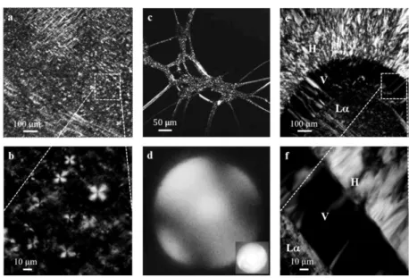
Afterward, in order to investigate the interaction between surfactant and water, a systematic experimental investigation of single paste droplets dissolution in static conditions will be performed. Differences between phases were highlighted using conoscopy image technique, and a dynamic rearrangement in the sample texture over time will be observed and
30
Subsequently, a home-made microfluidic device will be used to apply a well-controlled flow to the disc-shaped paste and, by time-lapse microscopy, dissolution time will be quantified. Firstly, different flow conditions will be tested using only pure water as a solvent, then, in order to modify the physical, chemical or rheological properties of the system, different solvents will be used, trying to understand the effect of chemical and mechanical stress on the process.
Subsequently, a medium scale experimental setup will be developed, this will be easier to use but also will be used to build a correlation between the results obtained with the microfluidic setup and tests that will be carried out in the pilot plant. To do this, a certain amount of SLES will be dissolved in a beaker using a blade agitator, testing the effect of stirring speed and concentration gradient. The dissolution process, in several conditions tested, will be monitored by measuring the value of the conductivity of the solution or of the Raman signal (both measured by means of probes that can be inserted directly in solution). From the fitting of the experimental data, a characteristic dissolution time will be extrapolated, specific for each speed and concentration condition.
Finally, a pilot plant scale set-up will be developed at the Procter & Gamble research center in Beijing. The operating conditions in which the tests will be carried out, similar to those used in the laboratory, and set up details will be described in chapter 4. As well as for the lab tests, from the experimental campaign conducted in the pilot plant, characteristic dissolution times for each various conditions will be taken out and these will be compared with the results obtained in the laboratory scale.
31
32
CHAPTER 1
Dissolution of concentrated surfactant solutions: from
microscopy imaging to rheological measurements
through numerical simulations.
Discussions contained in this chapter are under submission within: Rosa Ilaria Castaldo†, Rossana Pasquino†, Massimiliano M. Villone†, Sergio Caserta, Chong Gu, Nino Grizzuti, Stefano Guido, Pier Luca Maffettone, Vincenzo Guida. Dissolution of concentrated surfactant
solutions: from microscopy imaging to rheological measurements through numerical simulations. Chemical Engineering Journal.
33
Abstract
Many surfactants used in detergents experience complex phase and rheology changes when a thick paste is dissolved in water. During the dilution process, depending on water content, surfactant molecules can arrange in different morphologies, such as lamellas or cubic and hexagonal structures. These phases are characterized by different physicochemical properties, such as viscosity or diffusivity, which lead to non-simple transport mechanisms during the dissolution process.
In this work, we propose a multi-technique approach to investigate the dissolution of concentrated Sodium Lauryl Ether Sulfate (SLES) pastes in water under static and flow conditions. A thorough rheological characterization of the system showed non-monotonic changes of several orders of magnitude in its viscosity and viscoelastic moduli as a function of water content. Time-lapse microscopy allowed to image the dynamic evolution of the phase changes as water penetrated in a disk-shaped sample (with the same a geometry used in rheological tests). A simple diffusion-based multi-parameter model can describe satisfactorily both static and dynamic SLES dissolution data.
Introduction
SURFace ACTive AgeNTS (Surfactants) are molecules which have the ability to reduce the surface tension between a liquid, typically water, and another phase, favoring surface wettability, and miscibility with other liquids. They have high foaming, detergent, and solubilizing properties and it is for this reason that they are widely used in the personal-, home-, and beauty-care industry. Detergents and cosmetics are typically surfactant aqueous solutions18.
34
The industrial process for the preparation of commercial products typically involves mixing and dilution of originally highly concentrated surfactant pastes. At high concentration, surfactant molecules self-assemble into lyotropic mesophases exhibiting complex microstructure and rheology that are relevant for industrial processing1, 2. As concentration changes, molecules can rearrange, thus changing the microstructure of the system that in turn strongly affects the properties of the final product, which are determinant for its specific application. Therefore, it is necessary to identify and study the physicochemical processes involved in such transformations. Industrial processing of surfactant-based materials typically includes a water-dissolution step.
The dissolution of surfactant pastes presents some similarities with the polymer dissolution19, 20 but is made more difficult by the following aspects: 1) surfactant monomers form aggregates of variable size and shape that can vary with dilution and can dynamically form and disintegrate 2) the surfactant paste already contains the solvent (i.e. water), which makes the diffusion process “reversible” and more complex 3) the diffusion coefficient can be dependent in a non-monotonic way on the surfactant concentration, giving rise to multiple interfaces, difficult to be predicted. When a surfactant comes in contact with water, there is an inter-diffusion of the two molecular species, accompanied by the formation of mesophases9, which influence the evolution of the system during the dissolution process8, 21. It is well established that both physicochemical and rheological parameters, such as raw material chemistry, type of solvent, temperature and flow conditions, play a key role in the dissolution process3. However, the mechanisms governing the dissolution process are still not completely understood22, 23. This explains the great interest in the study
35
of the dissolution of complex molecules under static conditions and in flow2, 24-27, Understanding the dissolution of concentrated surfactant solutions in different solvents is of fundamental importance for their effective and wide industrial application.
The dissolution of surfactants in a solvent is diffusion-limited and, in general, can be described according to the diffusion layer model, in which two stages are observed: phase transition and diffusive transport. In order to fully understand the phenomenon of dissolution, then, one must have a good knowledge of the behavior of the equilibrium system. The equilibrium phase behavior of surfactant solutions has been extensively studied for different amphiphilic molecules and solvents28-30.
In this study, we consider Sodium Lauryl Ether Sulfate (SLES) as a model system. SLES is an anionic surfactant found in many categories of detergent products, e.g., soap, shampoo, and toothpaste, for its cheapness and effective foaming capacity. Recently, Poulos et al.1 have studied the dissolution of concentrate SLES in quiescent water through polarized light optical microscopy in both linear and circular geometries, finding bands with sharp interfaces. Their optical textures relate to cubic, hexagonal, and micellar phases appearing during the dilution of the concentrated surfactant. By tracking the movement of such bands, they have shown that dissolution can be modeled as a diffusive process and that it is possible to extract effective diffusion coefficients for each phase. In this work, we propose a multi-technique approach to investigate the SLES dissolution process both in static and flow conditions. We carry out a rheological characterization of the system in steady and oscillatory shear flow, a time-lapse-microscopy observation of phase-change evolution as water penetrates in a disk-shaped sample under static conditions, and finally we rationalize the two experimental contributions by a multi-parameter diffusive model, whose
36
parameter values give a satisfactory fit of both the rheological and microscopy data. To the best of our knowledge, static and dynamic dissolution experiments are here combined and rationalized under a unique framework for the first time.
Materials and methods
The surfactant used in our test is an Alkyl Ethoxy Sulphate (AES) paste provided by Procter and Gamble (Beijing, China). In particular, we will consider Sodium Lauryl Ether Sulfate (SLES, also known with its contract name Sodium Laureth 3 Sulfate, molecular weight = 288.38 g/mol31). A SLES concentrated paste 70%wt in water (density = 1.05 g/cm3 31) was available, and used without further purification. It is known that SLES in water can have a complex phase diagram, showing different morphologies. In particular, a Lamellar (L, 70-63%wt), Cubic (V1, 63-56%wt), Hexagonal (H, 56-31.5%wt) and Micellar phase (L1, 28-0.0236%wt) can be observed as a function of the concentration3. In the range 31.5-28%wt there is the coexistence of L1-H phases.
Aqueous solutions containing SLES ad different concentrations in the range 15-70%wt were prepared by adding the right amount of bi-distilled water to the concentrated raw paste. Equilibrium properties were reached by mixing samples with a magnetic stirrer for few days and continuous rheological tests were performed to prove stability over time.
Rheological setup
Rheological experiments were made with a stress-controlled rheometer (Physica, Anton Paar MCR702) equipped with a plate-plate geometry. In particular, frequency sweeps were performed at different concentrations in
37
the frequency range 100-0.1 rad/s in the linear regime (previously evaluated via strain sweep experiments). Flow curves were measured by tuning the shear rate in the range 100-0.01 s-1 by decreasing the sampling time at increasing shear rate.
The dissolution process was studied via a home-made plate-plate apparatus consisting of a water reservoir surrounding the surfactant paste mounted on a classical stress-controlled rheometer (Physica, Anton Paar MCR702), shown in Figure 8a. The raw paste was loaded between the rheometer plates, at time t = 0 water was added to the reservoir until reaching the total height of the plate-plate geometry (see schematic drawing in Figure 8a). A dynamic test at fixed frequency of 1 rad/s and low strain of 0.1% was performed at room temperature. The plate-plate gap was kept constant during the entire test. Two different plate-plate gaps (of 1 and 0.1 mm) and two different plate diameters (of 8 and 25 mm) were used in the experiments. During the dissolution process, the torque was monitored over time with the aim to relate its evolution to the morphological transitions arising in the sample.
Optical setup
Time-lapse microscopy was used to investigate SLES dissolution in water under static conditions. A microscope (Zeiss Axiovert 200, 10x and 20x objectives) was equipped with a high sensitivity CCD camera (Hamamatsu OrcaAG) and motorized stage, controlled by a home-made software, for automatic mosaic scanning of large samples32. The observation was done using two crossed polarizers, in order to visualize the internal microstructure. A tiny amount of raw surfactant paste ( 4 mg) was squeezed between the bottom glass of a home-made rectangular glass
38
chamber (12.5x8.5x2 cm) and a coverslip, obtaining a disk-shaped sample with an initial radius of about 4 mm. Sample thickness was set by inserting a double-side adhesive tape as a spacer between the two glass surfaces and measured to be 100 m. A fixed amount of water (15 ml) was added in the surrounding chamber at time t = 0 in order to induce sample dissolution. Experiments were run at room temperature ( 25°C). In Figure 8b, a sketch of the experimental setup is reported.
Figure 8 (Not to scale) schematic drawings of the rheological setup (a), the optical setup (b),
and of the computational domain for static dissolution numerical simulation (c).
Numerical model
In order to reproduce the experimental setup shown in Figure 8b, we considered a disk of 70%wt surfactant paste of initial radius R0 = 4 mm and
thickness h = 1 mm surrounded by a coaxial “cage” of (initially pure) water with radius Re = 24 mm. A (not to scale) schematic drawing of such system
is given in Figure 8c.
Given the axial symmetry and the absence of fluid convective motion, the system can be modeled by the transient mass balance equation on the surfactant in 1D along the radial direction. Assuming that the Fickian constitutive equation holds for the surfactant diffusion, the balance equation reads
39 𝜕𝑐 𝜕𝑡 = 1 𝑟 𝜕 𝜕𝑟[𝑟𝐷 𝜕𝑐 𝜕𝑟] (1)
where t is the time, r is the radial coordinate, c = c(r,t) is the (time- and position-dependent) surfactant molar concentration, and D = D(c) is the concentration-dependent diffusion coefficient of the surfactant. Expansion of Eq. 1 yields 𝜕𝑐 𝜕𝑡 = 𝜕𝐷 𝜕𝑟 𝜕𝑐 𝜕𝑟+ 𝐷 𝑟 𝜕𝑐 𝜕𝑟+ 𝐷 𝜕2𝑐 𝜕𝑟2 (2)
The model is supplied with the Boundary Conditions (BC)
𝜕𝑐
𝜕𝑟|𝑟=0= 0 (3)
𝑐|𝑟=𝑅e = 0 (4)
and the Initial Condition (IC)
𝑐|𝑡=0 = {𝑐0 ∀𝑟 ∈ [0, 𝑅0]
0 ∀𝑟 ∈]𝑅0, 𝑅e] (5)
Equation 3 expresses the axial symmetry at r = 0, whereas Eq. 4 gives the condition at r = Re. Strictly speaking, this would be valid at 𝑟 → ∞, but we
assumed it holds since Re >> R0 (and we verified it as explained in the
following). Finally, Eq. 5 is the initial condition on the whole domain, with the surfactant concentration being c0 = 0.7/MW (where MW is the
surfactant molecular weight) inside the disk and 0 outside.
In order to solve Eq. 2 with BCs 3-4 and IC 5, we discretized the domain into ns + nw intervals of length Δ𝑟 (bounded by ns + nw + 1 nodes) as shown
in Figure 8c, then we discretized Eq. 2 through the Finite Difference Method33. By choosing a second-order centered scheme for spatial
40
derivatives, from node 1 to node ns + nw - 1 the discretized mass balance
equation reads 𝜕𝑐𝑖 𝜕𝑡 = 𝐷𝑖−1 4Δ𝑟2(𝑐𝑖−1− 𝑐𝑖+1) + 𝐷𝑖+1 4Δ𝑟2(𝑐𝑖+1− 𝑐𝑖−1) + 𝐷𝑖 2𝑖Δ𝑟2[(2𝑖 + 1)𝑐𝑖+1− 4𝑖𝑐𝑖 + (2𝑖 − 1)𝑐𝑖−1] (6)
In node 0, the discretized Neumann BC reads
𝜕𝑐0
𝜕𝑡 =
4𝐷0
Δ𝑟2(𝑐1− 𝑐0) (7)
whereas in node ns + nw we have the Dirichlet BC
𝑐𝑛s+𝑛w = 0 (8)
At time 0, we imposed
𝑐𝑖 = { 𝑐0 ∀𝑖 = 0, … 𝑛s
0 ∀𝑖 = 𝑛𝑠+ 1, … , 𝑛𝑠+ 𝑛w (9)
Notice that in Eq. 6 also the diffusion coefficient D appears with a subscript, because, since we considered a dependence of such parameter on the surfactant concentration, in each node the Di-value depends on the ci-value.
In order to model this dependence, we assumed that each surfactant morphological phase is characterized by a specific value of the diffusion coefficient and that such value is constant for every concentration in that phase. In other words, in each node Di could attain one out of four different
values, depending on the phase (lamellar, hexagonal, cubic, or micellar) assumed by the surfactant.
Based on the above-mentioned assumptions, the model constituted by Eqs. 6-9 could be solved once the values of the three critical concentrations for phase transitions and of the four diffusion coefficients were chosen, yielding the numerically simulated time-varying radial profile of the
41
surfactant concentration in the domain shown in Figure 8c. From this, the numerical temporal trends of the radial positions of the three phase-transition fronts could be obtained. Such trends are shown and discussed below. We remark that preliminary space- and time-convergence test were performed, i.e., space- and time-discretization for the solution of Eqs. 6-9 were chosen as to ensure invariance of the numerical results upon further refinements, and that the water cage was large enough so that the condition imposed through Eq. 8 had no influence on the front displacements.
Results
Sample characterization
Figure 9 Viscosity curves for various SLES concentrations (see legend for details).
In Figure 9, steady viscosity data as a function of the shear rate are shown, parametric in SLES concentration. A Newtonian behavior is recorded when the surfactant concentration is low. As its concentration increases, the viscosity increases too and a shear thinning behavior can always be recorded, with the appearance in some cases of a yield stress. In addition, it
42
is apparent from Figure 9 that the viscosity increase at increasing SLES concentration is not monotonic.
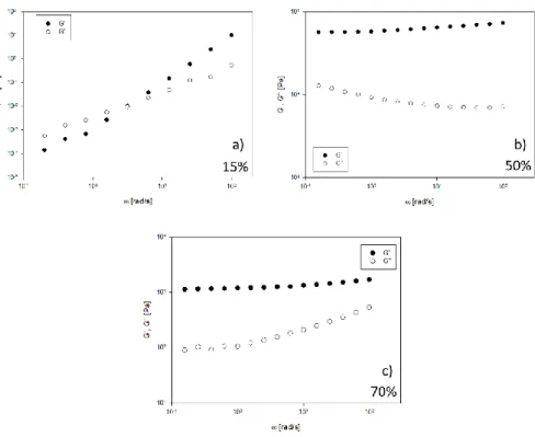
Figure 10 Viscoelastic moduli as function of angular frequency for 15%wt (a), 50%wt (b) and
70%wt (c) SLES.
Figure 10 shows the linear viscoelastic envelopes on samples containing
different SLES amounts. By tuning the concentration, it is possible to induce morphological transitions that, in turn, influence the rheological response. The most concentrated sample (70%wt) shows the peculiar response of a soft-solid-like material, with the elastic modulus overcoming the viscous one in the whole frequency range (see Figure 10c). A similar viscoelastic behavior is reported in Figure 10b for the 50%wt sample. Although counterintuitive, higher moduli than for the concentrated sample are recorded. On the other hand, the less concentrated sample (30%wt, see
well-43
defined cross-over frequency, which can be easily translated into a characteristic time for the micellar structure.
Figure 11 a) Magnitude of the complex viscosity at a frequency of 1 rad/s (black circles) and
steady viscosity at a shear rate of 1s-1 (white circles) as a function of SLES concentration. b) Elastic modulus (black circles) and loss modulus (white circles) at a frequency of 1 rad/s as a function of SLES concentration. The dashed lines represent morphological transitions: L1
micellar phase, H hexagonal phase, V1 cubic phase, La lamellar phase.
In order to understand how the rheological response of the sample depends on SLES concentration, i.e. what is the relation between structure and rheology, and also to verify the applicability of the Cox-Merz rule, Figure
11 reports the overlay between the magnitude of the complex viscosity and
the steady viscosity at a specific angular frequency/shear rate (panel a) and the viscoelastic moduli at a specific angular frequency (panel b) as function of the SLES concentration. Morphological transitions, whose values have been identified by vertical lines, according to the thermodynamic phase diagram3, have been marked with vertical dashed lines and different letters have been used to label the incoming microstructures (see legend for details). Some information arises from Figure 11: (i) it is actually possible to detect phase transitions via rheological methods, (ii) rheological parameters are non-monotonic with SLES concentration: the maxima correspond to cubic and hexagonal phases, whereas the lower levels of viscosity and moduli are related to the micellar phase, (iii) the Cox-Merz rule is not valid (as expected), except for the micellar phase; the magnitude
44
of the complex viscosity, which depicts equilibrium properties, is always higher than the steady viscosity, as flow can strongly influence the sample microstructure, (iv) except for L1, all the other morphologies show a
pronounced elastic response.
Optical experiments
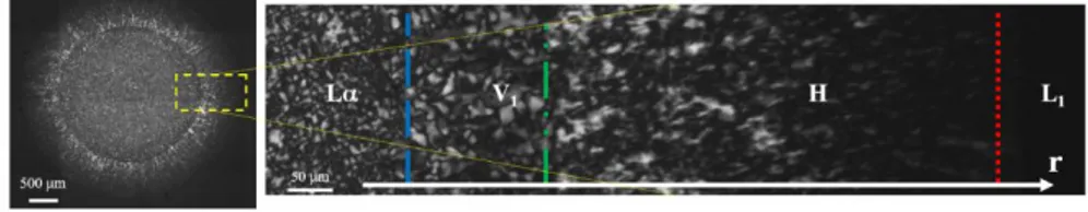
In this section, we report the results of the time-lapse microscopy analysis of the dissolution process made using the optical experimental setup described above. After adding water into the chamber (at t = 0), the surfactant paste that is confined between the two glass surfaces (see Figure
8b) came in touch with the solvent and started to dissolve. Water penetrated
radially changing the sample concentration and its microstructure. In Figure
12, we report on the left a mosaic scanning of the entire disk paste acquired
in polarized light during the dissolution process. On the right, a zoom of a radial section of the same image is reported. The sample shows an onion-like radially layered structure and it is possible to identify four different regions, in agreement with the SLES phase diagram. A L core is surrounded by two concentric shells (V1 and H), while the external phase is
a micellar solution (L1) that appears completely black because it is not
birefringent. The boundaries between the phases are clearly visible and highlighted with different lines in the zoom on the right: the blue dashed line separates the lamellar core from the cubic layer (L-V1), the green
dash-double-dot line identifies the boundary between the cubic layer and the hexagonal shell (V1-H), finally the red dotted line identifies the external
boundary between the hexagonal and the micellar phase (H-L1). The
line-color code is in agreement with the rheological phase diagram reported in
45
Figure 12 Optical experiments. During the dissolution of a surfactant disk, it is possible to
visualize 4 different phases: an internal core of lamellar phase (L ), a first ring of cubic phase (V1), a second ring of hexagonal phase (H), and a more external micellar phase (L1). The
interfaces between the phases shrink radially as dissolution goes on.
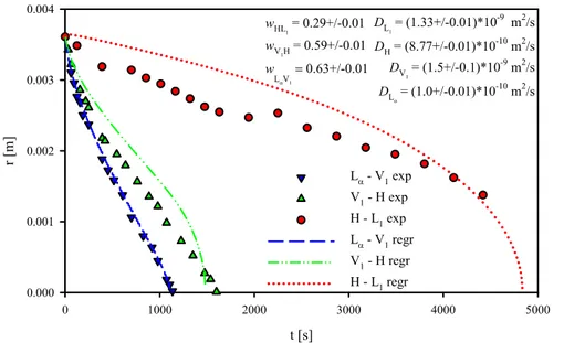
The time evolution of interface positions was measured by image analysis techniques. As time passed, the three boundaries shrank toward the center of the sample, so that at the end of the experiment the surfactant paste was dissolved, leaving only a black micellar solution. During the experiment, the distances of the interfaces from the center of the surfactant disk were manually identified. In Figure 13, the radial displacement of the 3 fronts is reported as a function of time. Red dots, up green triangles and down blue triangles identify the H-L1, V1-H, and Lα-V1 transition, respectively. As the
dissolution process went on, the radial position of the interfaces decreased down to zero, when the inner phase disappears. It is evident that the time evolutions of the two “internal” interfaces (L-V1 and V1-H) are “faster”
than the external interface (H-L1). This means that the entire process is
controlled by the “slow” external transition between the hexagonal and the micellar phase. In our experimental conditions, when the lamellar and cubic phases had disappeared, the hexagonal phase sample was still about half of its original size.
46
Figure 13 Radial displacements of the La-V1, V1-H, and H-L1 phase-transition fronts during
the dissolution of a 4-mm-radius 70%wt surfactant disk. Symbols: experimental measurements; Curves: Least Squares fits by a Fickian diffusion model (the estimated
parameters reported in the legend).
Experimental data fit
In order to find the values of the phase-transition concentrations and of the diffusion coefficients yielding the experimentally measured front displacements reported in Figure 12 (and to validate the simple model based on Fickian diffusion depicted above), we performed a fit of the experimental data in Figure 13 based on the model presented in Sec. 2. In order to do that, as there is no analytical expression for the front displacements as a function of the parameters, we applied an iterative procedure, namely, we numerically solved the linear system given by Eqs. 6-9 repeatedly at varying the values of the 7 parameters in appropriate ranges, then we “selected” the parameter set for which the sum of the squared differences between the experimental and the numerical data was the minimum. The ranges in which we made the phase-transition concentrations and the diffusion coefficients
47
vary during such procedure were selected on the basis of the literature on SLES3. The red, green, and blue lines in Figure 13 are the H-L
1, V1-H, and
L-V1 phase-transition front displacements arising from the simulation for
which the parameters are such that the sum of the squared differences between the experimental and the numerical data is minimized. A satisfactory agreement holds between the experimental and the numerical data, thus providing a measure of the phase-transition concentrations and of the diffusion coefficients in our system and validating its description through a simple model based on Fickian diffusion. The values of the 3 phase-transition concentrations (in terms of surfactant mass fraction) and of the diffusion coefficients in the 4 phases yielding the curves reported in
Figure 13 are displayed on the top right. Of course, since we made the
parameter values vary discretely, the precision of our estimate of the fitting parameters is affected by the incremental steps of the variations we imposed. It is worth mentioning that the order of magnitude of the diffusion coefficients estimated here is consistent with that of the effective diffusion coefficients estimated by Poulos et at.1 through a different approach. In
Figure 15 in the SI, analogous optical measurements as in Figure 13 are
reported for two samples with different initial surfactant concentration, i.e., 50%wt and 60%wt, and compared with numerical fitting.
Dynamic rheological experiments
In this section, we report the results of the analysis of the dissolution process, using the rheological experimental setup described above.
Transient experiments were carried out with a 70%w/w surfactant paste. Here, we will consider only one specific example, performed isothermally in a plate-plate geometry with plate radius Ri = 4 mm and the gap between
48
the plates of height h = 0.1 mm. In order to monitor the torque evolution after the addition of (initially pure) water in a controlled geometry, we made a time-sweep test in the linear regime. The experimental results are shown in Figure 12 along with data from numerical simulations, that will be presented afterward. The torque is reported as a function of time: at very low times, the water addition creates a transient oscillation, which is related to the time needed by the sample rim to reach equilibrium. After the first minimum, the evolution of the torque can be considered as a measure of the dissolution process, by means of the diffusive water in the surfactant paste. The torque passes through a well-defined maximum and then decreases towards significantly lower values. The rise can be explained by comparing
Figure 13 with Figure 11, where increasing time results in a decrement in
concentration. The maximum can be, then, explained with a morphological transition from the lamellar phase (70%wt surfactant paste) to a cubic/hexagonal phase, whereas the abrupt decrease of the torque depicts the transition to the micellar phase, which is characterized by very low viscoelastic moduli, as already discussed in the previous section.
In order to simulate the dynamic rheological experiment described above, we considered a plate-plate rheometer of plate radius Ri = 4 mm with the
gap between the plates (of height h = 0.1 mm) initially filled with a 70%wt surfactant paste. The rheometer plates were surrounded by a concentric pool of (initially pure) water with radius Re = 24 mm and height hw slightly
greater than h undergoing Small Amplitude Oscillatory Shear (SAOS) flow. Hence its upper plate was subjected to rotation back and forth with velocity 𝑣𝜃(𝑟, 𝑡) = 𝛾0(𝑟)𝜔 cos(𝜔𝑡) ℎ (10)
where 0(r) is the radially-dependent oscillation amplitude, = 1/2 s-1 is
49
𝛾0(𝑟) = 𝛾0,max 𝑟
𝑅i (11)
with 0,max = 0.001 the (small) maximum oscillation amplitude (i.e., the
oscillation amplitude at the plate border).
If the surfactant paste is modeled as a linear viscoelastic liquid, the shear felt by the liquid under SAOS flow can be expressed as24
𝜎(𝑟, 𝑡) = 𝛾0,max 𝑟
𝑅𝑖[𝐺
′(𝑐(𝑟, 𝑡)) sin(𝜔𝑡) + 𝐺′′(𝑐(𝑟, 𝑡)) cos(𝜔𝑡)] (12)
where G’ and G’’ are the elastic and viscous moduli, respectively. Notice that, as shown by the experimental data in Figure 11b, both G’ and G’’ depend on surfactant concentration, which, in turn, depends on space and time, since, while the rheometer undergoes its oscillatory motion, the surfactant diffuses as discussed above. (We assume that, as the SAOS flow is slow, it provides no additional (convective) mechanism to surfactant dissolution in the flow cell, thus the latter can be entirely ascribed to Fickian diffusion. Therefore, the torque felt by the rheometer rotating plate is 𝑀(𝑡) = ∫ 𝜎(𝑟, 𝑡)2𝜋𝑟𝑑𝑟 = 2𝜋𝑅i 0 𝛾0,max 𝑅i [sin(𝜔𝑡) ∫ 𝐺 ′(𝑐(𝑟, 𝑡))𝑟3𝑑𝑟 𝑅i 0 + cos(𝜔𝑡) ∫ 𝐺𝑅i ′′(𝑐(𝑟, 𝑡))𝑟3𝑑𝑟 0 ] (13)
In order to calculate M(t), we interpolated the G’(c)- and G’’(c)-experimental data in Figure 10b through piecewise cubic Hermite polynomials, then we combined such information with the c(r,t)-field arising from the solution of Eqs. 6-9 with the parameters obtained by fitting the optical measurements of the front displacements, as detailed above. We made use of this information to compute the right-hand side in Eq. 13. In Figure 14, the experimental and numerical values of the maximum of the torque absolute value max |M| are reported as function of time, showing
50
that, as the surfactant paste dissolution goes on during the SAOS flow, the torque at the upper plate first increases, it reaches a maximum, then it decreases until becoming barely measurable. In terms of both the t- and max |M|-scales, a good agreement holds between the numerical and experimental points.
Figure 14 Maximum of the torque modulus |M| measured by the parallel plate rheometer
during the dissolution of a 4-mm-radius surfactant disk. Pink circles: experimental measurements, cyan triangles: numerical simulations
Conclusions
In this paper, we propose a multi-technique approach to investigate the dissolution of Sodium Lauryl Ether Sulfate (SLES) in water both in static and flow conditions.
We performed a rheological characterization of the system under steady and oscillatory shear flow that showed non-monotonic changes of several orders
51
of magnitude in its viscosity and viscoelastic moduli as a function of surfactant concentration.
Time-lapse-microscopy observations on a disk-shaped SLES sample in quiescent water showed water penetrating radially, thus making the sample assume an onion-like radially layered structure where each layer was characterized by a microstructure typical of a different mesophase.
We developed a simple diffusion-based multi-parameter model, by means of which we were able to describe satisfactorily static and dynamic SLES dissolution data at the same time.
The results obtained using the different experimental and numerical approaches are all in great agreement, showing for the first time a comprehensive analysis of the dissolution phenomena of complex surfactant pastes under static and flow conditions. The approach here proposed can provide useful support to the design and optimization of several industrial processes.
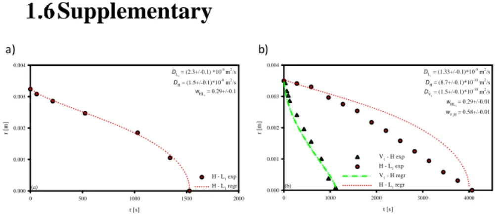
Supplementary
Figure 15 Radial displacements of the phase-transition fronts during the dissolution of a
4-mm-radius surfactant disk paste with an initial concentration equal to 50%wt (a) and 60%wt (b). Symbols: experimental measurements, curves: Least Squares fits by a Fickian diffusion model (the estimated parameters are reported in each panel on the right).
In Figure 15, analogous optical measurements as in Figure 13 are reported for two samples with different initial surfactant concentration, i.e., 50%wt (panel a) and 60%wt (panel b). In Figure 15a, the paste was initially in the
t [s] 0 500 1000 1500 2000 r [m ] 0.000 0.001 0.002 0.003 0.004 H - L 1 exp H - L1 regr D L1 = (2.3+/-0.1) *10 -9 m2/s D H = (1.5+/-0.1)*10 -9 m2/s w HL1 = 0.29+/-0.1 (a) t [s] 0 1000 2000 3000 4000 r [m ] 0.000 0.001 0.002 0.003 0.004 V 1 - H exp H - L1 exp V 1 - H regr H - L1 regr D L1 = (1.33+/-0.1)*10 -9 m2/s D H = (8.7+/-0.1)*10 -10 m2/s DV1 = (1.5+/-0.1)*10 -10 m2/s wHL1 = 0.29+/-0.01 w V1H = 0.58+/-0.01 (b) a) b)