Our reference: COMPHY 5258
P-authorquery-v11
AUTHOR QUERY FORM
Journal:
Computer Physics Communications
Article Number: 5258
Please e-mail or fax your responses and any corrections to:
E-mail: [email protected]
Fax: +44 1392 285879
Dear Author,
Please check your proof carefully and mark all corrections at the appropriate place in the proof (e.g., by using on-screen annotation
in the PDF file) or compile them in a separate list. Note: if you opt to annotate the file with software other than Adobe Reader then
please also highlight the appropriate place in the PDF file. To ensure fast publication of your paper please return your corrections
within 48 hours.
For correction or revision of any artwork, please consult
http://www.elsevier.com/artworkinstructions
.
Location
in article
Query / Remark
click on the Q link to go
Please insert your reply or correction at the corresponding line in the proof
Q1
Please confirm that given names and surnames have been identified correctly.
Please check this box or indicate
your approval if you have no
corrections to make to the PDF file
Thank you for your assistance.
Computer Physics Communications xx (xxxx) xxx–xxx
Contents lists available atScienceDirect
Computer Physics Communications
journal homepage:www.elsevier.com/locate/cpcA framework for building hypercubes using MapReduce
Q1 ∧D.
∧Tapiador
a,∗,
∧W.
∧O’Mullane
a,
∧A.G.A.
∧Brown
b,
∧X.
∧Luri
c,
∧E.
∧Huedo
d,
∧P.
∧Osuna
a aScience Operations Department, European Space Astronomy Centre, European Space Agency, Madrid, SpainbSterrewacht Leiden, Leiden University, P.O. Box 9513, 2300 RA Leiden, The Netherlands cDepartament d’Astronomia i Meteorologia ICCUB-IEEC, Marti i Franques 1, Barcelona, Spain
dDepartamento de Arquitectura de Computadores y Automática, Facultad de Informática, Universidad Complutense de Madrid, Spain
a r t i c l e i n f o
Article history: Received 26 July 2013 Received in revised form 17 November 2013 Accepted 4 February 2014 Available online xxxx Keywords: Hypercube Histogram Data mining MapReduce Hadoop Framework Column-oriented Gaia mission
a b s t r a c t
The European Space Agency’s Gaia mission will create the largest and most precise three dimensional chart of our galaxy (the Milky Way), by providing unprecedented position, parallax, proper motion, and radial velocity measurements for about one billion stars. The resulting
∧
catalogwill be made available to the scientific community and will be analyzed in many different ways, including the production of a variety of statistics. The latter will often entail the generation of multidimensional histograms and hypercubes as part of the precomputed statistics for each data release, or for scientific analysis involving either the final data products or the raw data coming from the satellite instruments.
In this paper we present and analyze a generic framework that allows the hypercube generation to be easily done within a MapReduce infrastructure, providing all the advantages of the new Big Data analysis paradigm but without dealing with any specific interface to the lower level distributed system implementation (Hadoop). Furthermore, we show how executing the framework for different data storage model configurations (i.e. row or column oriented) and compression techniques can considerably improve the response time of this type of workload for the currently available simulated data of the mission.
In addition, we put forward the advantages and shortcomings of the deployment of the framework on a public cloud provider, benchmark against other popular solutions available (that are not always the best for such ad-hoc applications), and describe some user experiences with the framework, which was employed for a number of dedicated astronomical data analysis techniques workshops.
© 2014 Published by Elsevier B.V.
1. Introduction
1
Computer processing capabilities have been growing at a fast 2
pace following Moore’s law, i.e. roughly doubling every two years 3
during the last decades. Furthermore, the amount of data man-4
aged has been also growing at the same time as disk stor-5
age becomes cheaper. Companies like Google, Facebook, Twitter, 6
LinkedIn, etc. nowadays deal with larger and larger data sets which 7
need to be queried on-line by users and also have to answer busi-8
ness related questions for the decision making process. As instru-9
mentation and sensors are basically made of the same technology 10
as computing hardware, this has happened as well in science as we 11
∗Corresponding author. Tel.: +34 686028931.
E-mail addresses:[email protected](D. Tapiador),
[email protected](W. O’Mullane),[email protected] (A.G.A. Brown),[email protected](X. Luri),[email protected](E. Huedo), [email protected](P. Osuna).
can discern in projects like the human genome, meteorology infor- 12 mation and also in astronomical missions and telescopes like Gaia 13 [1], Euclid [2], the Large Synoptic Survey Telescope – LSST [3] or 14 the Square Kilometer Array – SKA [4], which will produce data sets 15 ranging from a petabyte for the entire mission in the case of Gaia 16 to 10 petabytes of reduced data per day in the SKA. 17 Furthermore, raw data (re-)analysis is becoming an asset for 18 scientific research as it opens up new possibilities to scientists 19 that may lead to more accurate results, enlarging the scientific 20 return of every mission. In order to cope with the large amount of 21 data, the approach to take has to be different from the traditional 22 one in which the data is requested and afterwards analyzed (even 23 remotely). One option is to move to Cloud environments where one 24 can upload the data analysis work flows so that they run in a low- 25 latency environment and can access every single bit of information. 26 Quite a lot of research has been going on to address these 27 challenges and new computing paradigms have lately appeared 28 such as NoSQL databases, that relax transaction constraints, or 29 other Massively Parallel Processing (MPP) techniques such as 30
http://dx.doi.org/10.1016/j.cpc.2014.02.010 0010-4655/©2014 Published by Elsevier B.V.
MapReduce [5]. This new architecture emphasizes the scalability 1
and availability of the system over the structure of the information 2
and the savings in storage hardware this may produce. In this 3
way the scale-up of problems is kept reasonably close to the 4
theoretical linear case, allowing us to tackle more complex 5
problems by investing more money in hardware instead of making 6
new software developments which are always far more expensive. 7
An interesting feature of this new type of data management system 8
(MapReduce) is that it does not impose a declarative language 9
(i.e. SQL), but it allows users to plug in their algorithms no 10
matter the programming language they are written in and let 11
them run and visit every single record of the data set (always 12
brute force in MapReduce, although this may be worked around if 13
needed by grouping the input data in different paths using certain 14
constraints). This may also be accomplished to some extent in 15
traditional SQL databases through User Defined Functions (UDFs) 16
although code porting is always an issue as it depends a lot on the 17
peculiarities of the database and debugging is not straightforward 18
[6]. However, scientists and many application developers are more 19
experienced at, or may feel more comfortable with, embedding 20
their algorithms in a piece of software (i.e. a framework) that sits 21
on top of the distributed system, while not caring much about what 22
is going on behind the scenes or about the details of the underlying 23
system. 24
Furthermore, some of the more widely used tools in data mining 25
and statistics are multidimensional hypercubes and histograms, as 26
they can provide summaries of different and complex phenomena 27
(at a coarser or finer granularity) through a graphical representa-28
tion of the data being analyzed, no matter how large the data set 29
is. These tools are useful for a wide range of disciplines, in partic-30
ular in science and astronomy, as they allow the study of certain 31
features and their variations depending on other factors, as well as 32
for data classification aggregations, pivot tables confronting two 33
dimensions, etc. They also help scientists validate the generated 34
data sets and check whether they fit within the expected values of 35
the model or the other way around (also applicable to simulations). 36
As multidimensional histograms can be considered a very 37
simple hypercube which normally contains one, two or three 38
dimensions (often for visualization purposes) and whose measure 39
is the count of objects given certain concrete values (or ranges) 40
of its dimensions, we will generally refer to hypercubes through 41
the paper and will only mention histograms when the above 42
conditions apply (hypercubes with one to three dimensions whose 43
only measure is the object count). 44
Previous work applying MapReduce to scientific data includes 45
[7], where a High Energy Physics data analysis framework is em-46
bedded into the MapReduce system by means of wrappers (in the 47
Map and Reduce phases) and external storage. The wrappers en-48
sure that the analytical algorithms (implemented in a different 49
programming language) can natively read the data in the frame-50
work specific format by copying it to the local file system or to 51
other content distribution infrastructures outside the MapReduce 52
platform. Furthermore, [8] and [9] examine some of the current 53
public Cloud computing infrastructures for MapReduce and study 54
the effects and limitations of parallel applications porting to the 55
Cloud respectively, both from a scientific data analysis perspec-56
tive. In addition, [10] shows that novel storage techniques being 57
currently used in commercial parallel DBMS (i.e. column-oriented) 58
can also be applied to MapReduce work flows, producing signifi-59
cant improvements in the response time of the data processing as 60
well as in the compression ratios achieved for randomly-generated 61
data sets. Last but not least, several general-purpose layers on top 62
of Hadoop (i.e. Pig [11] and Hive [12]) have lately appeared, aim-63
ing at processing and querying large
∧
data setswithout dealing di-64
rectly with the lower level API of Hadoop, but using a declarative 65
language that gets translated into MapReduce jobs. 66
Fig. 1. Star density map using HEALPix.
This paper is structured as follows. In Section2, we present the 67 simulated data set that will be used through the paper and some 68 simple but useful examples that can be built with the framework. 69 Section3describes the framework internals. In Section4, we show 70 the experiments carried out, analyzing the deployment in a public 71 Cloud provider, examining the data storage models (including 72 the column-oriented approach) and compression techniques, and 73 benchmarking against two other well known approaches. Section5 74 puts forward some user experiences in some astronomical data 75 analysis techniques workshops. Finally, Sections6and7refer to 76 the conclusions and future work respectively. 77
2. Data analysis in the Gaia mission 78
In the case of the Gaia mission, many histograms will be 79 produced for each data release in order to summarize and 80 document the
∧
catalogsproduced. Furthermore, a lot of density 81
maps will have to be computed, e.g. for visualization purposes, as 82 otherwise it would be impossible to plot such a large amount of 83 objects. All these histograms and plots (see [13] for examples), the 84 so-called precomputed statistics, will have to be (re)generated in the 85 shortest period of time and this will imply a load peak in the data 86
∧
center. Therefore, the solution adopted should be able to scale to 87 the Cloud just in case it is needed due to e.g. the absence of a local 88 infrastructure that can execute these work flows (as it would mean 89 a high fixed cost for hardware which is underutilized most of the 90
time). 91
Figs. 1 and2 show two simple examples of histograms that 92
have been created with the framework and which we will use 93 throughout the paper for presenting the different results obtained. 94 The GUMS10 data set [13], from which histograms have been 95 created, is a simulated
∧
catalogof stars that resembles the one that 96 will be produced by the Gaia mission. It contains a bit more than 97 two billion objects with a size of 343 GB in its original delivery form 98 (binary and compressed with Deflate). Since there is no Gaia data 99 yet, all Gaia data processing software is verified against simulated 100 observations of this universe model [13]. 101 The histogram shown inFig. 1is a star density map of the sky. It 102 has been built by using a sphere tessellation (pixelization) frame- 103 work named HEALPix [14], which among other things provides a 104 set of routines for subdividing a spherical surface into equal area 105 pixels, and for obtaining the pixel number corresponding to a given 106 pair of angular coordinates. HEALPix is widely known not only in 107 astronomy but also in the field of earth observation. HEALPix also 108 allows indexing of geometrical data on the sphere for speeding up 109 queries and retrievals in relational databases. The resolution of the 110 pixels is driven by a parameter called Nside, which must be a power 111 of two. The higher this parameter is, the more pixel subdivisions 112 the sphere will have. For Nside
=
1024 (used inFig. 1and in the 113 rest of tests below) there are 12 582 912 pixels. 114D. Tapiador et al. / Computer Physics Communications xx (xxxx) xxx–xxx 3
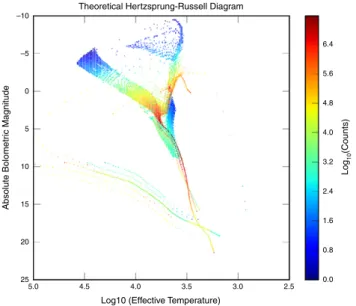
Fig. 2. Theoretical Hertzsprung–Russell diagram. The horizontal axis shows the
temperature of the stars on a logarithmic scale and the vertical axis shows a measure of the luminosity (intrinsic brightness) of the stars (also logarithmic, brighter stars are at more negative values).
The example in Fig. 2 is a theoretical Hertzsprung–Russell 1
diagram (two dimensional) which shows the effective temperature 2
of stars vs. their luminosity. This is a widely used diagram in 3
astronomy, which contains information about the age (or mixture 4
of ages) of the plotted set of stars as well as about the physical 5
characteristics and evolutionary status of the individual stars. 6
For the scenario just sketched the MapReduce approach is the 7
most reasonable one. This is not only due to the fact that it scales up 8
very well (also in the Cloud) or that there are open-source solutions 9
already available like Hadoop1(which we will use), but also
be-10
cause the generation of a hypercube fits perfectly into the MapRe-11
duce paradigm. This is not necessarily true for other parallel com-12
puting paradigms such as Grid computing, where the processing is 13
efficiently distributed but the results are cumbersome to aggregate 14
afterwards, or MPI,2where the developer has to take care of the 15
intrinsic problems of a distributed system. In the case of a parallel 16
DBMS, these two simple examples could be easily created either 17
by using UDFs with external HEALPix libraries (something already 18
done for Microsoft SQL Server at the Sloan Digital Sky Survey3) or 19
directly with a SQL query for the theoretical Hertzsprung–Russell 20
diagram. However, more complex histograms or hypercubes 21
would be much more difficult to generate. Furthermore, the scal-22
ability will be better in Hadoop as the data set grows due to the 23
inherent model of MapReduce. Last but not least, the generation of 24
several histograms and/or hypercubes each one with different con-25
straints in terms of filtering or aggregation (e.g. several star density 26
maps at different Nsidegranularities) will be more efficient using
27
our framework on top of Hadoop (provided the amount of data is 28
very large) as they will be computed in one single scan of the data. 29
3. Framework description
30
The framework (implemented in Java) has been conceived 31
considering the following features: 32
•
Thin layer on top of Hadoop that allows users or external tools 33to focus only on the definition of the hypercubes to compute. 34
1http://hadoop.apache.org. 2www.mpi-forum.org. 3http://www.sdss.org/.
•
Hide all the complexity of this novel computing paradigm and 35 the distributed system on which it runs. Therefore, it provides 36 a way to deal with a cutting-edge distributed system (Hadoop) 37 without any knowledge of Big Data internals. 38•
Possibility to process as many hypercubes as possible in one sin- 39 gle scan of data, taking advantage of the brute-force approach 40 used in Hadoop jobs, thus reducing the time for generating the 41 precomputed statistics required for each data release. 42•
Leverage the capabilities offered by this new computing model 43 so that the solution is scalable. 44•
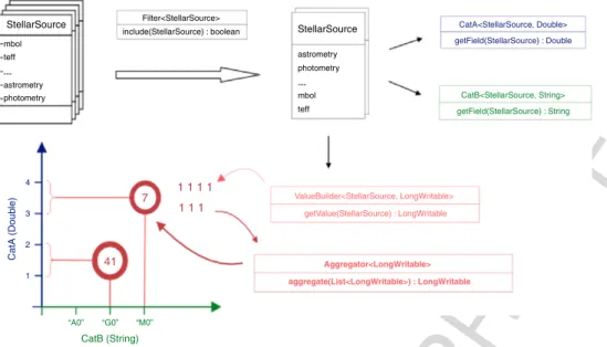
Java generics have been used throughout the framework in order 45 to ease its integration in any domain and permit a straightfor- 46 ward embedding of any already existing source code. 47 Hypercubes defined in the framework (seeFig. 3for an exam- 48 ple) may have as many dimensions (categories) as required. They 49 may define intervals (for a continuous function) or be of a dis- 50 crete type (for discrete functions), depending on the use case. Users 51 may supply their own algorithms in order to specify how the value 52 of each dimension will be computed (by implementing the corre- 53 sponding getField method). This value might be of a custom user- 54 defined type in case of need. The input object being processed at 55 each time is obviously available for performing the relevant calcu- 56lations. 57
It is important to highlight that the possibility of defining as 58 many dimensions as needed is what allows us to easily build data 59 mining hypercubes or concrete pivot tables, and do so on-the- 60 fly (at runtime) without losing generality. This is a key feature 61 for scientific data analysis because the data is always exploited 62 in many different ways due to the diversity of research studies 63 that can be done with them. Furthermore, the cubes generated 64 may be further analyzed (i.e. slice, dice, drill-down and pivoting 65 operations) within the framework by defining a new Hadoop 66 input format that reads the output of the cube generation job 67 and delivers it to the next analytical job. The results can also be 68 exported to a database in order to perform the subsequent analysis 69
in there. 70
We must also set the value that will be returned for each entry 71 being analyzed. This will usually be a value of ‘1’ when performing 72 e.g. counts of objects falling into each combination of categories, 73 but it might also be any other derived (user-implemented) quan- 74 tity for which we want to know the maximum or minimum value, 75 the average, the standard deviation, or any other linear statistical 76 value. There is only one MapReduce phase for the jobs so more 77 complex statistics cannot currently be calculated, at least not ef- 78 ficiently and in a scalable way (e.g. the median, quartiles and the 79 like). We may however define a custom type such that the cells of 80 the hypercube contain more information than just a determined 81 measure. We can also define a filter which is used to decide which 82 input objects will be analyzed and which ones will be discarded for 83 each hypercube included in the job. 84 The current implementation offers a lot of helpers that can be 85 plugged in many different places for many different purposes. For 86 instance, if we just want to get a field out of the input object 87 being processed for a certain dimension (or for the value returned), 88 we can just use a helper reader that obtains that field at runtime 89 through Java reflection, and avoid the generation of a new class 90 whose only method would just return the field. The user just needs 91 to specify the field name and make sure that the object provides the 92 relevant accessor (getter method). 93 Last but not least, the manner in which the data is aggregated 94 as well as whether the aggregator can be used as the Hadoop 95 combiner for the job (recommended whenever possible [15]) can 96 also be defined by the user (and could also be defined per 97 hypercube with minor changes), although most of the time they 98 will just set one of the currently available helpers (for computing 99 counts, the minimum/maximum value, the average, the standard 100
Fig. 3. Data workflow through the framework and main interfaces to implement for each hypercube. The sample in the figure shows a hypercube with two dimensions
(discrete for the x axis and continuous with intervals for the y axis) that counts the number of elements falling into each combination of the categories.
deviation, etc.). For more complex hypercubes (i.e. several 1
measures aggregated differently on each cell of the hypercube), we 2
could create an aggregator along with a custom type for cell values 3
so that the different measures are aggregated differently (the count 4
for some of them, the average for others, etc.). 5
Before running the job it is required to set some configuration 6
properties for the definition of the input files and the correspond-7
ing input format to use, the path where to leave the results, the 8
class that will define the hypercubes to create (Listing 1 shows the 9
skeleton of this class for the example shown inFig. 3), and some 10
other parameters like the type of the output value returned for 11
them (mandatory for any Hadoop job). This last constraint forces 12
all entities computed in the same job to have the same return 13
type (the reducer output value, e.g. the count, the maximum value, 14
etc.), although this can be easily worked around if needed by set-15
ting more generic types (a Double for holding both integers and 16
floating point numbers, a String for numbers and text, etc.), or as 17
stated above, developing a custom type (implementing the Hadoop 18
Writable interface) that holds them in different fields, along with
19
the corresponding aggregator. 20
Listing 1: Custom class defining the hypercube(s) to compute. 21
p u b l i c c l a s s MyHypercubeBuilder
22
extends BuilderHelper < S t e l l a r S o u r c e , LongWritable > {
23 24 @Override 25 p u b l i c L i s t <Hypercube< S t e l l a r S o u r c e , LongWritable >> 26 getHypercubes ( ) { 27
// Create list holding the hypercubes
28
// Create CatA instance (with ranges)
29
// Create CatB instance
30
// Create Filter instance
31
// Create ValueBuilder (use Helper)
32
// Create Aggregator (use Helper)
33
// Create Hypercube instance
34
// Add to hypercubes list
35
// Return hypercubes list
36 } 37 38 } 39 40
The output files of the job have two columns, the first one 41
for identifying the hypercube name as well as the combination 42
of the concrete values for its dimensions (split by a separator 43
defined by the user), and the second one holding the actual value 44
of that combination of categories (see Listing 2 for a sample of 45
the output for the Theoretical Hertzsprung–Russell diagram shown 46 inFig. 2). The types used for discrete categories must provide a 47 method to return a string which unequivocally identifies each of 48 the possible values of the dimension. For categories with intervals, 49 the string in the output file will contain information on the interval 50 itself with square brackets and parentheses as appropriate (closed 51 and open ends respectively), but again they must ensure that 52 the types of the interval ends (bin ends) supply a unequivocal 53 string representation. This unequivocal representation might be 54 the primary key of the dimension’s concrete value (for more 55 advanced hypercubes) so that it can later on be joined with the rest 56 of the information of that dimension as it usually happens in data 57
mining star schemas. 58
Listing 2: Sample of the output for the Theoretical Hertzsprung– Russell diagram shown in Fig. 2.
59 [ . . . ] 60 TheoreticalHR / [ 3 . 5 8 , 3 . 5 8 2 5 ) / [ 1 6 . 7 , 1 6 . 7 2 5 ) / 998 61 TheoreticalHR / [ 3 . 5 8 , 3 . 5 8 2 5 ) / [ 8 . 0 , 8 . 0 2 5 ) / 883 62 TheoreticalHR / [ 3 . 5 8 7 5 , 3.59)/[−4.875 ,−4.85)/ 328 63 TheoreticalHR / [ 3 . 5 8 7 5 , 3.59)/[−5.4 ,−5.375)/ 391 64 TheoreticalHR / [ 3 . 6 0 7 5 , 3.61)/[−0.9 ,−0.875)/ 87031 65 TheoreticalHR / [ 3 . 6 0 7 5 , 3.61)/[−3.6 ,−3.575)/ 2780 66 TheoreticalHR / [ 3 . 6 0 7 5 , 3.61)/[−3.925 ,−3.9)/ 12384 67 [ . . . ] 6869
One straightforward but important optimization that has been 70 implemented is the usage of sorted lists for dimensions that de- 71 fine continuous, non-overlapping intervals. This way the number 72 of comparisons to do per input object is considerably lowered, 73 reducing by a factor of 20 the time taken for the execution. There- 74 fore, although non-continuous (and non-ordered) interval cate- 75 gories are allowed in the framework, it is strongly recommended 76 to define continuous (and non-overlapping) ranges even though 77 some of them may be later on discarded. 78
4. Experiments 79
4.1. Cloud deployment 80
Recently there has been a blossoming of commercial Cloud 81 computing service providers, for example Amazon Web Services 82 (AWS), Google Compute Engine, Rackspace Cloud, Microsoft Azure 83
D. Tapiador et al. / Computer Physics Communications xx (xxxx) xxx–xxx 5
and several other companies or products sometimes focused on 1
different needs (Dropbox, Google Drive, etc.). AWS has become 2
one of the main actors in this Cloud market, offering a wide 3
range of services such as the ones that have been used for 4
this work: Amazon Elastic MapReduce (Amazon EMR4), Amazon 5
Simple Storage Service (Amazon S35) and Amazon Elastic Compute
6
Cloud (Amazon EC26). The way these three services are used is as
7
follows: EC2 provides the computers that will run the work flows, 8
S3 is the data store where to take the data and leave the results, 9
and EMR is the Hadoop ad-hoc deployment (and configuration) 10
provided for MapReduce jobs. Amazon charges for each service, 11
and not only for the computing resources but also for the storage 12
on S3 and the data transfers in and out of their infrastructure. They 13
also provide different instances (on-demand, reserved and spot 14
instances) which obviously have different prices at different levels 15
of availability and service. The EMR Hadoop configuration is based 16
on the current operational version of Hadoop with some bug fixes 17
included. Furthermore, the overall experience with Amazon EMR 18
is very good and it has been quite easy to start submitting jobs to 19
it through command line tools openly available. Debugging is also 20
quite easy to do as ssh access is provided for the whole cluster of 21
nodes. 22
The deployment used for testing and benchmarking consists of 23
eight worker nodes each one having the Hadoop data and task 24
tracker nodes running on them. There is also one master node 25
which runs the name node and the job tracker. The AWS instance 26
chosen is m1.xlarge, which has the following features: 27
•
4 virtual cores (64-bit platform). 28•
15 GB of memory. 29•
High I/O performance profile (1 Gbps). 30•
1690 GB of local Direct Attached Storage (DAS), which sums 31up to a bit more than 13 TB of raw storage which may be cut 32
down by half or more depending on the Hadoop Distributed File 33
System (HDFS) [16] replication factor chosen. 34
With this layout, EMR Hadoop deployment launches a maxi-35
mum number of 8 mappers and 3 reducers per worker node (64 36
and 24 for the entire cluster respectively). It is important to re-37
mark that the time taken for starting the tasks of a job in Hadoop is 38
not negligible (more than one minute for the tests carried out) and 39
certainly affects the performance of short jobs [6], as it imposes a 40
minimum amount of time that a job will always last (sequential 41
workload) no matter the amount of data to process. This is one of 42
the reasons why Hadoop is mostly advised for very big workloads 43
(Big Data), where this effect can just be disregarded. 44
4.2. Data storage model considerations
45
Scientific raw data sets are not normally delivered in a 46
uniformly sized set of files as the parameters chosen for placing 47
the data produce a lot of skew due to features inherent to the 48
data collection process (some areas of the sky are more densely 49
populated, a determined event does not occur at regular intervals, 50
etc.). This is also true for the data set being analyzed in this paper 51
(GUMS10) as it comprises a set of files each one holding the 52
sources of the corresponding equal-area sky region (seeFig. 1for 53
its histogram drawn in a sky projection). This may be a problem 54
for binary (and often compressed) files when stored in HDFS as 55
the records cannot be split into blocks (there is no delimiter as 56
in the text format). The data formats studied in this paper are of 57
4http://aws.amazon.com/elasticmapreduce/. 5http://aws.amazon.com/s3/.
6http://aws.amazon.com/ec2/.
Fig. 4. Performance for different HDFS block and file sizes (files in GBIN format are
binary and compressed with Deflate).
this type (binary and compressed with no delimiters), defined by 58 the Gaia mission SOC (Science Operations Centre). Thus we have 59 to read each of them sequentially in one Hadoop mapper and their 60 size must be roughly the same and equal to the defined HDFS 61 block size to maximize performance through data locality.Fig. 4 62 shows the performance obtained when computing the different 63 histograms shown inFigs. 1and2: a HEALPix density map and a 64 theoretical Hertzsprung–Russell diagram. As we can see, once we 65 group the data into equally sized files and set the HDFS block to 66 that size, the time consumed for generating them is approximately 67 2
/
3 the time taken when the original highly-skewed delivery is 68 used. The standard format chosen for data deliveries within the 69 Gaia mission is called ‘GBIN’, which contains Java-serialized binary 70 objects compressed with Deflate (ZLIB). 71In Fig. 4 we can also see that there is a block size which 72
performs slightly better than the others (512 MB) which is a 73 consequence of the concrete configuration used for the testbed, 74 as more files mean more tasks (Hadoop mappers) being started 75 which is known to be slow in Hadoop as already remarked above. 76 Furthermore, less but bigger files may produce a slowdown in the 77 data shuffling period (each Hadoop mapper outputs more data 78 which then has to be combined and shuffled). Therefore, we will 79 use the best configuration (data files and block size of 512 MB) 80 for the comparison with other data storage techniques and for 81
benchmarking. 82
To analyze the effects of the different compression techniques 83 available and study how they perform for an astronomical data set, 84 a generic data input format has been developed. This way, different 85 compression algorithms and techniques may be plugged into 86 Hadoop, again without dealing with any Hadoop internals (input 87 formats and record readers). This is more or less the same idea as 88 the generic input format interface provided by Hadoop but more 89 focused on binary (non-splittable) and compressed data. The data 90 reader to use for the job must be configured through a property 91 and its implementation must provide operations for setting up 92 and closing the input stream to use for reading, and for iterating 93 through the data objects. The readers developed so far store Java 94 serialized binary objects with different compression techniques 95 which are indicated below as: GBIN for Deflate (ZLIB), Snappy for 96 Google Snappy7compression and Plain for no compression. 97
Fig. 5shows the results obtained when these compression tech- 98 niques are used with the GUMS10 data set for creating the same 99 histograms as before. It is important to remark that no atten- 100 tion has been paid to other popular serialization formats currently 101 available like Thrift,8Avro9etc., as the time to (de)serialize is al- 102 ways negligible compared to the (de)compression one. Further- 103 more, as stated above, the data is always stored in binary format as 104 the textual counterpart would lead to much worse results (a proof 105 of this is the battery of tests presented in [6]). 106
7http://code.google.com/p/snappy/. 8http://thrift.apache.org/. 9http://avro.apache.org/.
Fig. 5. Data storage model approaches performance comparison.
Fig. 6. Data set size for different compression and format approaches.
Google Snappy codec gives a much better result as the decom-1
pression is faster than Deflate (GBIN). It takes half of the time to 2
process the histograms (50%) and the extra size occupied on disk 3
is only around 23% (see Fig. 6). This confirms the suitability of 4
this codec for data to be stored in HDFS and later on analyzed by 5
Hadoop MapReduce work flows. 6
Fig. 5 also shows the performance obtained with another
7
data storage model developed ad-hoc using a new Hadoop input 8
format, column-oriented (see the rightmost two columns in both 9
histograms), which resembles the one presented in [10], although 10
it integrates better in the client code as the objects returned are 11
of the relevant type (the information that we want to populate 12
from disk still has to be statically specified though as in [10]). 13
Furthermore, we obviously expect that the improvements made 14
by the column input format are more significant as the data set 15
grows larger (both in number of rows and columns), although we 16
can also state that performance will decrease when most of the 17
data set columns are required in a job, due to overheads incurred 18
in the column-oriented store mechanism (several readers used at 19
the same time, etc.). These issues have to be carefully considered 20
for each particular use case before any of the formats is chosen. 21
The Hadoop operational version at the time of writing does not 22
yet provide a way to modify the block data placement policy when 23
importing data into HDFS (newer alpha/beta versions do support 24
this to some extent although these could not be used in Amazon 25
EMR). The current algorithm for deciding what data node is used 26
(whenever an input stream is opened for a certain file), chooses 27
the local node if there is a replica in there, then another random 28
node in the same rack (containing a replica) if it exists, and if 29
there is no one serving that block in the same rack it randomly 30
chooses another data node in an external rack (containing a replica 31
of course). Considering this algorithm, if we set the replication 32
policy to the number of cluster worker nodes, we ensure that there 33
will always be a local replica of everything on every node and thus 34
we can simulate that the column files corresponding to the same 35
data objects have been placed in the same data node (and replicas) 36
for data locality of input data readers. This is not to be used in an 37
operational deployment of course, but it has served its purpose in 38 our study. Meanwhile, new techniques that overcome these issues 39 are being put in place (i.e. embed data for all columns in the same 40
file, and split by row ranges). 41
These new techniques, whose main implementations are 42 Parquet,10ORC11(Optimized Row Columnar) and Trevni12(already 43 discontinued in favor of Parquet) should always be chosen instead 44 of ad-hoc developments like the one presented here, as even 45 though some of them may not yet be ready for operations, they 46 are rapidly evolving and will become very soon the default input 47 and output formats for many use cases, overall for those found in 48 science and engineering. The main features of this new technique 49
are enumerated below: 50
•
Data are stored contiguously on disk by columns rather than 51 rows. Then, each block in HDFS contains a range of rows of the 52∧
data setand there is some metadata that can be used to seek 53
to the start or the end of any column data, so if we are reading 54 just two columns, we
∧
do nothave to scan the whole block, but 55
just the two columns data. This way, it is not necessary to create 56 many different files which might incur in extra overhead for the 57
HDFS name node. 58
•
Compression ratio for each column data will be higher than 59 the row oriented counterpart due to the fact that values 60 for the same column are usually more similar, overall for 61 scientific data sets involving time series, because new values 62 representing certain phenomena are likely to be similar than 63 those just measured. These implementations go beyond a 64 simple compression for the column data by allowing different 65 compression algorithms for different types of data, or even do so 66 on the fly as we create the∧
data setby trying several alternatives. 67 For instance, for a column representing a measure (floating 68 point number) of a determined sensor or instrument, it would 69 be reasonable to use a delta compression algorithm where 70 we store the differences between values which will probably 71 require less bits for their representation. It is important to 72 remark that I/O takes more time than the associated CPU 73 time (de)compressing the same data. For other columns with 74 enumerated values, the values themselves will be stored in the 75 metadata section along with a shorter (minimum) set of bits 76 which will be the ones being used in the column data values. 77 This of course requires (de)serializing the whole block (range of 78 rows) for building back the original values of each column, but 79 this technique usually performs well and takes less time. 80
10http://parquet.io/.
11 http://docs.hortonworks.com/HDPDocuments/HDP2/HDP-2.0.0.2/ds_Hive/ orcfile.html.
D. Tapiador et al. / Computer Physics Communications xx (xxxx) xxx–xxx 7
•
Predicate push-down. Not only we can specify the set of1
columns that will be read for a determined workflow, but for 2
those that need to be queried or filtered with some constraints, 3
we can also push down the predicates so that the data not 4
needed are not even deserialized in the worker nodes, or even 5
not read from disk (only the metadata available is accessed). 6
•
Complex nested data structures can be represented in the 7format (not just simple flattening of nested namespaces). The 8
technique for implementing this feature is presented in more 9
detail in [17]. 10
•
This data format representation is agnostic to the data process-11ing, data model or even the programming language. 12
•
Further improvements of the column-based approach include 13the ability to split files without scanning for markers, some kind 14
of indexing for secondary sorting, etc. 15
Fig. 6shows that the level of compression achieved by our naive 16
implementation of the column-oriented approach (compared to 17
the row-oriented counterpart) is not as good as it might be 18
expected. This may be caused by the fact that an entire row may 19
much resemble the next row (similar physical properties), so the 20
whole row may be considered a column, but at a higher granularity, 21
leading to a relatively good compression in the row-oriented 22
storage model as well. Another more plausible explanation for this 23
may be that we do not use deltas for adjacent data (in columns) as 24
is usual [18], but the values themselves. 25
Contrasting the results inFigs. 5and6, we see that the column-26
oriented storage model (using Snappy codec) takes more disk space 27
than the row-oriented one (with Deflate). This extra cost overhead 28
(64 GB) amounts to $8 per month in Amazon S3 storage (where 29
the data are taken from at cluster initialization time), which is 30
much less than the price incurred in a typical workload where 31
many histograms and hypercubes have to be computed, as e.g. the 32
cluster must be up 24 min more in the case of a HEALPix density 33
map computation (which comes to a bit more than $3 extra per 34
job) or 25 min more for a single theoretical Hertzsprung–Russell 35
diagram (again a bit more than $3 extra per job). Therefore, for 36
typical larger workloads of several (and more complex) histograms 37
and/or hypercubes, we can expect larger and larger cost savings 38
with the column-oriented approach as computation is much more 39
expensive than the extra overhead in S3 storage, mainly due to the 40
amount of jobs to be run as well as the non-negligible cost of the 41
cluster nodes. 42
4.3. Benchmarking
43
Two powerful and well-known products have been chosen for 44
the benchmark, Pig130.11.0 and Hive140.10.0. These open source
45
frameworks, which also run on top of Hadoop, offer an abstraction 46
of the MapReduce model, providing users with a general purpose, 47
high-level language that could be used not only for the hypercubes 48
described above, but also for other data processing workflows such 49
as ETL (Extract, Transform and Load). However, they might require 50
some further work to do in case we wanted to build more complex 51
hypercubes (involving several dimensions and values, some of 52
them computed with already existing custom code), or generating 53
several hypercubes in one scan of the input data (something not 54
neatly expressed in a SQL query). 55
The tests carried out use a row-oriented scheme with com-56
pressed (Snappy) binary data and have been run on the infrastruc-57
ture described in Section4.1. For the purpose of benchmarking, we 58
will carefully analyze different scenarios: 59
13http://pig.apache.org/. 14http://hive.apache.org/.
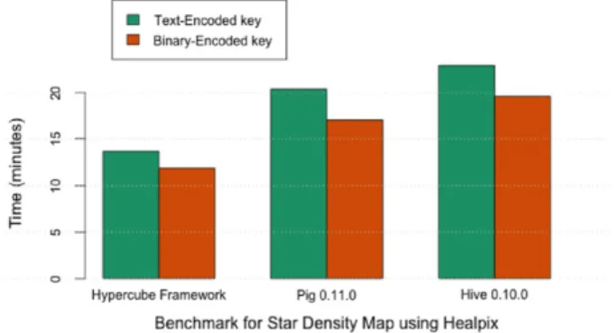
Fig. 7. Comparison among the framework presented and other popular data analysis tools currently available. All tests have been run using the Hadoop standard Merge-Sort algorithm for data aggregation.
•
Simple one-dimensional hypercube with the key encoded as 60 text (the default for the framework), and as binary (more 61efficient but less flexible). 62
•
Two-dimensional hypercube with low key cardinality where 63 the aggregation factor is high. 64•
Several hypercubes at the same time with different key 65cardinalities. 66
•
Different aggregation algorithms (default Merge Sort and Hash- 67based). 68
•
Scalability tests by increasing the∧
data setsize, but keeping the 69
same cardinalities for the keys. 70
Fig. 7shows the results obtained when generating the hyper- 71
cube plotted inFig. 1. Two approaches (with the key encoded as 72 text and as binary) have been considered in order to prove that the 73 proportions in execution time for the different solutions are kept, 74 although the framework is supposed to always work with text in its 75 current version. We can see that the framework performs consid- 76 erably better (33% in the case of Pig and up to 40% for Hive) and we 77 argue that this may be due to its simplicity in the design yet the ef- 78 ficient core logic built inside, which cannot be achieved by general 79 purpose frameworks that are supposed to span a very wide domain 80 of applications. Therefore, this generality has a high impact in cost 81 when we focus on a particular use case like the one described here. 82 The results shown in Fig. 8 refer to the scalability of the 83 alternatives studied for different computations and configurations. 84 The same
∧
data set (GUMS10) is used to enlarge the input size, 85
although it is important to notice that the output size will remain 86 the same as the number of bins will not change as we increase the 87
input data. 88
We can see that the framework performs significantly better in 89 the use cases studied, which proves that for well-known, opera- 90 tional workloads, it is usually better to use a custom implementa- 91 tion (or an ad-hoc framework) rather than using general purpose 92 tools which are more suited for exploration or situations where 93 performance is not so important. However, we can be certain that 94 these general purpose and higher level implementations are catch- 95 ing up fast enough if we look at the optimizations they are cur- 96 rently releasing, such as hash-based aggregation. This technique 97 (known as In-Mapper combiner) tries to avoid data serialization 98 and disk I/O by aggregating data in a hash table in memory. Then, 99 the mappers that run in the same JVM do not emit data until they 100 are all finished (as long as the aggregation ratio is high enough). 101 Then, the steps for serializing data and the associated disk I/O 102 before the combiner is executed are not needed anymore, thus im- 103 proving performance dramatically. The logic built-in for accom- 104 plishing this new functionality is rather complex not only because 105 Hadoop was not designed for this kind of processing in the first 106 place, but also due to the dynamic nature of the implementations, 107 which can switch on-the-fly between hash-based and merge-sort 108
(a) Star density map using HEALPix (one dimension). (b) Theoretical Hertzsprung–Russell diagram (two dimensions).
(c) Star density map using HEALPix at eight different resolutions (one dimension, eight different hypercubes in the same run).
Fig. 8. Scalability benchmark for (a) star density map, (b) theoretical HR diagram and (c) star density map at eight different resolutions. The approaches shown encompass
different alternatives from the Hadoop ecosystem and the two main algorithms used for aggregating data, i.e. Merge Sort (the default for Hadoop) and Hash Aggregation (whose implementation is known in the Hadoop ecosystem as In-Mapper combiner). The results for Hash aggregation are only shown for Hive, which is the only one that showed some improvements in the tests run. The
∧
data setis enlarged one, two and four times with the same data (1×GUMS10, 2×GUMS10 and 4×GUMS10 respectively) and therefore the cardinality of the key space for each hypercube being computed remains unchanged.
aggregations by spilling to disk what is inside the hash table once 1
a certain configured aggregation threshold is not met by the work-2
flow at run time. The implementation of this automatic switching 3
is something that will make these higher level tools much more ef-4
ficient, but it will also require much more expertise from users for 5
tuning the best configuration for the workflows. 6
Furthermore, the current implementation for Hive shows a very 7
good performance gain as shown inFig. 8(c) but is not significantly 8
better than the merge-sort counterpart when using Hadoop 9
directly. This may be caused by the fact that there is not much I/O 10
due to the small size of each pair of keys and values, compared to 11
the savings produced for a better in-memory aggregation. Results 12
for hash-based aggregation in Pig have been omitted due to its 13
very poor performance in the release used, which proves that a 14
more robust implementation must properly handle the memory 15
consumed by the hash table, allowing to switch to Merge Sort 16
dynamically whenever the cardinality goes beyond a predefined 17
threshold. This dynamism in query execution may become an asset 18
for Hadoop-based processing comparing to parallel DBMS, where 19
the query planner picks one alternative at query parsing time and 20
usually sticks to it till the end. In Hadoop, this is more dynamic and 21
gives more flexibility and adaptability at run time. 22
One of the most common features of data pipelines is that they 23
are often DAG (Directed Acyclic Graph) and not linear pipelines. 24
However, SQL focuses on queries that produce a single
∧
result set. 25
Thus, SQL handles trees such as joins naturally, but has no built 26
in mechanism for splitting a data processing stream and applying 27
different operators to each sub-stream. It is not uncommon to 28
find use cases that need to read one data set in a pipeline and 29
group it by multiple different grouping keys and store each as 30
separate output. Since disk reads and writes (both scan time and 31
intermediate results) usually dominate processing of large data 32
sets, reducing the number of times data must be written to and 33 read from disk is crucial to good performance. 34 The recent inclusion of the GROUPING SETS clause in Hive 35 has also contributed to the improvements shown in Fig. 8(c), 36 comparing to those in Fig. 8(a) and (b), as it allows that the 37 aggregation is made with different keys (the ones specified in the 38 clause) yet only one scan of data is needed. This fits perfectly in the 39 scenario posed in the test shown inFig. 8(c), where we compute 40 several hypercubes at the same time in the same
∧
data set. However, 41
GROUPING SETS clause is complex since the keys specified have to 42 be in separate columns. Therefore, when trying to compute results 43 in the format of a single key plus its corresponding value, we will 44 always get the key which the row refers to, plus the rest of keys 45
with empty values (null). 46
We have found other usability issues in Hive, which we believe 47 will be addressed soon, but which may currently lead to a worse 48 user experience, such as the lack of aliases on columns. This is a 49 minor problem, but most of the users and client applications are 50 used to relying on them everywhere for reducing complexity or 51 increasing flexibility, overall when applying custom UDF or other 52 built-in operators. Furthermore, there is no way to pass parameters 53 to the UDF when initializing, which has made the execution of 54 the multi-hypercube workflow more difficult to run, as several 55 different UDF had to be coded, even though they all share the same 56 functionality and the only difference is the parameter that sets the 57
resolution of the map. 58
Comparing Pig and Hive, results show that Pig performs 59 significantly better than Hive when the (Hadoop) standard Merge 60 Sort algorithm is chosen. However, the implementation of the 61 hash-based aggregation in Hive seems more mature and gives a 62 better performance than the Merge Sort alternative in Hive, for 63 those cases where the aggregation factor is high enough (see the 64
D. Tapiador et al. / Computer Physics Communications xx (xxxx) xxx–xxx 9
tendency ofFig. 8(b) where the aggregation factor is increased as 1
we enlarge the
∧
data setdue to the same data being duplicated). 2
One of the most important conclusions to take away when look-3
ing at these results is that there is no solution that fits all problems. 4
Therefore, special care has to be taken when choosing the product 5
to use as well as when setting the algorithm and tuning its param-6
eters. Results show that a bad decision may even double execu-7
tion time for certain workloads. In this case, an ad-hoc solution fits 8
better than more generic ones, even though already implemented 9
hash-based algorithms in Hive and Pig may seem more appropri-10
ate upfront. In addition, there are other optimizations that could 11
be easily made, such as sort avoidance, because it is normally not 12
needed when processing aggregation workflows. 13
Another remark worth mentioning is that when we double 14
the input size, the execution time is a bit less than the expected 15
(double) one. This is due to the fact that Hadoop inherent overhead 16
starting jobs is compensated by the larger workload, which proves 17
that Hadoop is not well suited for small
∧
data setsas there is a non-18
negligible (and well-known) latency starting tasks in the worker 19
nodes. 20
5. User experience
21
The hypercube generation framework is packaged as a JAR (Java 22
Archive) file and has a few
∧
dependenceson other packages (mainly 23
on those of Hadoop distribution). To make use of the framework, 24
the user has to write some code that sets what hypercubes to 25
compute (see Listing 1), as well as any extra code that will be 26
executed by the framework, e.g. when computing the concrete 27
categories or values for each hypercube and input record in the 28
∧
data set being processed. Furthermore, the user is expected to 29
package all classes into a JAR, create a file containing (at least) the 30
properties specified in Section3(input and output paths, etc.), and 31
run that JAR on a Hadoop cluster following Hadoop documentation. 32
The framework has been tested by offering it to a variety of 33
user groups. One of the authors (AB), without any background in 34
computer science (but with experience in Java programming), tried 35
out the framework as it was being developed. He had no significant 36
problems in understanding how to write pieces of Java code needed 37
to generate hypercubes for specific categories or intervals and 38
was able to quickly write a small set of classes for supporting the 39
production of hypercubes for quantities (e.g. energy and angular 40
momentum of stars) that involve significant manipulation of the 41
basic
∧
catalogquantities. How to write additional filters based on 42
these quantities was also straightforward to comprehend. 43
Subsequently the framework (together with the small set of 44
additional classes) was offered to students attending a school 45
on the science and techniques of Gaia. During this school the 46
students were asked to produce a variety of hypercubes (such as 47
the ones inFigs. 1and2) based on a subset of the GUMS10 data 48
set. The aim was to give the attendants a feel for working with 49
data sets corresponding to the Big Data case. The programming 50
experience of this audience (mostly starting Ph.D. students) ranged 51
from almost non-existent, to experience with procedural and 52
scripting languages, to very proficient in Java. Hence, although the 53
conceptual parts of the framework were not difficult to understand 54
for the students (what is a hypercube, what is filtering, etc.), the 55
lack of knowledge in both the Java programming language, and in 56
its philosophy and methods proved to be a significant barrier in 57
using the framework. 58
Widespread opinions were for instance: ‘‘Given the Java pro-59
gramming language learning curve the framework is a huge 60
amount of work for short term studies but is very useful for long 61
term and more complex studies’’ and ‘‘Java needs a complete 62
change of mind with respect to the way we are used to program-63
ming’’. The framework was also offered at a workshop on simulat-64
ing the Gaia catalogue data and there the attendants consisted of 65
a mix of junior and senior astronomers. The reactions to the use of 66 the framework were largely the same. 67 On balance we believe that once the language barrier is 68 overcome the framework provides a very flexible tool to work with. 69 The way of obtaining the data and the fact that the user may choose 70 the treatment of these data, enables a wide range of possibilities 71 with regard to scientific studies based on the data. 72 The fact that it operates under a Hadoop system makes it an 73 efficient way of serving data analysis of huge amounts of data with 74 respect to conventional database systems, due to the nature of the 75 requests presented by the users in the seminars: ‘‘They must be 76 completely customizable for any statistics or studies a scientist 77 wanted to develop with the source data’’. 78 Another interesting point is the way the data is presented on 79 output. It can be parsed with any data mining software that can 80 represent graphical statistical data due to its simple representa- 81 tion, and it can also be understood by the users themselves without 82
major issues. 83
6. Conclusions 84
In this paper, we have presented a framework that allows us to 85 easily build data mining hypercubes. This framework fills the gap 86 between the computer science and scientific (e.g. astrophysical) 87 communities, easing the adoption of cutting-edge technologies for 88 accomplishing new scientific research challenges not considered 89 before. In this respect the framework adds a layer on top of 90 the Hadoop MapReduce infrastructure so that scientific software 91 engineers can focus on the algorithms themselves and forget about 92 the underlying distributed system. The latter provides a new way 93 of working with big data sets such as the ones that will be produced 94 by ESA’s Gaia mission (only simulations currently available). 95 Furthermore, we explored the suitability of current commercial 96 Cloud deployments for these types of work flows, analyzed the 97 application of novel data storage model techniques currently 98 being exploited in parallel DBMS (i.e. column-oriented storage) 99 and benchmark the solution against other popular data analysis 100 techniques on top of Hadoop. On one hand, the column orientation 101 has proven to be very effective for the generation of hypercubes 102 as the number of columns involved in the process is often much 103 less than the ones available in the original data set (the facts table 104 in a data mining star schema), especially in scientific contexts 105 where each study often focuses on a very specific area (astrometry 106 or photometry in the astrophysical field for instance). On the 107 other hand, the fact that the framework focuses on a specific 108 field (generation of hypercubes), makes it better in terms of 109 performance than other well-known solutions like Pig and Hive 110 under the same conditions for the data processing. We argue that 111 this is one aspect that must always be considered (tradeoff of the 112 generality
∧
vs. performance) as too generic solutions may penalize 113 performance as they need more logic inside to cope with the 114 variety of features they provide. 115 In addition, we show several results that suggest the architec- 116 ture to be considered for binary data in Hadoop work flows and 117 conclude that it is always better to compress the data set as the CPU 118 time for decompression is much less than the extra I/O overhead 119 for reading the uncompressed counterpart. We also prove that light 120 compression techniques, such as Snappy, are more suited for ana- 121 lytical work flows than more aggressive compression techniques 122 (which are aimed at increasing data transfer rates). 123 Last but not least, the framework can also be used in any 124 other discipline or field, as it is very common to use hypercubes 125 (and pivot tables) for summarizing big data sets, or for providing 126 business intelligence capabilities. Using the framework in other 127 disciplines can be done without losing its generality (much needed 128 due to the diversity of studies that can be made with scientific data 129
7. Future work
1
There are several lines of work that have been opened by this 2
research, including: 3
•
Extensions or internal optimizations of the framework. 4•
Benchmarking against other possible solutions such as the ones 5provided in the data mining extensions of commercial (parallel) 6
DBMS, or other solutions being currently developed within 7
the Hadoop ecosystem which aim at providing near-real time 8
responses for queries that return small data sets. 9
•
Use other already existing implementations of the column-10based approach and benchmark against the improvements 11
already made with more naive implementations. 12
Some possible extensions are the ability to automatically use 13
data coming from different sources by joining and filtering them 14
in a first MapReduce phase with the user-supplied field and 15
constraints respectively, and computing the hypercube requested 16
in a subsequent phase. This would be ideal for raw data analysis. 17
Furthermore, another internal optimization might be to use binary 18
types instead of text for the keys when the hypercubes are simple 19
enough (as shown in the benchmark), as the usage of long text 20
strings can cause a slowdown in the sorting, hashing and shuffling 21
stages. 22
The framework’s efficiency should be benchmarked and com-23
pared to new technologies that aim at producing near-real time 24
responses by both working in memory as much as possible, and 25
by pulling the intermediate results of the internal computations 26
directly from memory instead of disk. These tests should not only 27
focus on the speedup and scale-up, but also analyze different work-28
loads involving geometry and time series. This comparison should 29
also take into account the different data storage model layouts de-30
scribed in this paper (particularly the column input format), as well 31
as the data aggregation ratio for each particular hypercube (and the 32
best algorithms to apply in each case). 33
Acknowledgments
34
This research was partially supported by Ministerio de Ciencia 35
e Innovación (Spanish Ministry of Science and Innovation), 36
through the research grants TIN2012-31518, AYA2009-14648-37
C02-01 and CONSOLIDER CSD2007-00050. The GUMS simulations 38
were run on the supercomputer MareNostrum at the Barcelona 39
Supercomputing Center—Centro Nacional de Supercomputación. 40
References 41
[1] F. Mignard, Overall science goals of the Gaia mission, in: C. Turon, K.S. O’Flaherty, M.A.C. Perryman (Eds.), ESA SP-576: The Three-Dimensional Universe with Gaia, 2005, pp. 5–+.
42
[2] Euclid. Mapping the geometry of the dark Universe, Definition Study Report, Tech. rep., European Space Agency/SRE, July, 2011.
43
[3] Z. Ivezic, J.A. Tyson, LSST: from science drivers to reference design and 44
anticipated data products. ArXiv e-printsarXiv:0805.2366. 45
[4] P. Dewdney, P. Hall, R. Schilizzi, T. Lazio, The square kilometre array, Proc. IEEE 97 (8) (2009) 1482–1496.
46
[5] J. Dean, S. Ghemawat, MapReduce: simplified data processing on large clusters, Commun. ACM 51 (1) (2008) 107–113.
47
[6] A. Pavlo, E. Paulson, A. Rasin, D.J. Abadi, D.J. DeWitt, S. Madden, M. Stonebraker, A comparison of approaches to large-scale data analysis, in: Proceedings of the 2009 ACM SIGMOD International Conference on Management of Data, SIGMOD’09, ACM, New York, NY, USA, 2009, pp. 165–178.
48
[7] J. Ekanayake, S. Pallickara, G. Fox, MapReduce for data intensive scientific analyses, in: Proceedings of the 2008 Fourth IEEE International Conference on eScience, ESCIENCE’08, IEEE Computer Society, Washington, DC, USA, 2008, pp. 277–284.
49
[8] T. Gunarathne, T.-L. Wu, J. Qiu, G. Fox, MapReduce in the Clouds for science, in: 50
2010 IEEE Second International Conference on Cloud Computing Technology 51
and Science, CloudCom, 2010, pp. 565–572. 52
[9] S.N. Srirama, O. Batrashev, P. Jakovits, E. Vainikko, Scalability of parallel scientific applications on the Cloud, Sci. Program. 19 (2–3) (2011) 91–105.
53
[10] A. Floratou, J.M. Patel, E.J. Shekita, S. Tata, Column-oriented storage techniques for MapReduce, Proc. VLDB Endow. 4 (7) (2011) 419–429.
54
[11] A.F. Gates, O. Natkovich, S. Chopra, P. Kamath, S.M. Narayanamurthy, C. Olston, 55
B. Reed, S. Srinivasan, U. Srivastava, Building a high-level dataflow system 56
on top of Map-Reduce: the Pig experience, Proc. VLDB Endow. 2 (2) (2009) 57
1414–1425. URLhttp://dl.acm.org/citation.cfm?id=1687553.1687568. 58
[12] A. Thusoo, J.S. Sarma, N. Jain, Z. Shao, P. Chakka, S. Anthony, H. Liu, P. Wyckoff, 59
R. Murthy, Hive: a warehousing solution over a Map-Reduce framework, Proc. 60
VLDB Endow. 2 (2) (2009) 1626–1629. 61
URLhttp://dl.acm.org/citation.cfm?id=1687553.1687609. 62
[13] A.C. Robin, X. Luri, C. Reylé, Y. Isasi, E. Grux, S. Blanco-Cuaresma, F. Arenou, C. Babusiaux, M. Belcheva, R. Drimmel, C. Jordi, A. Krone-Martins, E. Masana, J.C. Mauduit, F. Mignard, N. Mowlavi, B. Rocca-Volmerange, P. Sartoretti, E. Slezak, A. Sozzetti, Gaia Universe model snapshot, A&A 543 (2012) A100.
63
[14] K.M. Grski, E. Hivon, A.J. Banday, B.D. Wandelt, F.K. Hansen, M. Reinecke, M. Bartelmann, HEALPix: a framework for high-resolution discretization and fast analysis of data distributed on the sphere, Astrophys. J. 622 (2) (2005) 759.
64
[15] Y. Kwon, M. Balazinska, B. Howe, J. Rolia, A study of skew in MapReduce applications, in: 5th Open Cirrus Summit, 2011.
65
[16] K. Shvachko, H. Kuang, S. Radia, R. Chansler, The Hadoop distributed file 66
system, in: 2010 IEEE 26th Symposium on Mass Storage Systems and 67
Technologies (MSST), 2010, pp. 1–10. 68
[17] S. Melnik, A. Gubarev, J.J. Long, G. Romer, S. Shivakumar, M. Tolton, T. 69
Vassilakis, Dremel: interactive analysis of web-scale datasets, in: Proc. of the 70
36th Int’l Conf on Very Large Data Bases, 2010, pp. 330–339. 71
URLhttp://www.vldb2010.org/accept.htm. 72
[18] J. Krueger, M. Grund, C. Tinnefeld, H. Plattner, A. Zeier, F. Faerber, Optimizing write performance for read optimized databases, in: Proceedings of the 15th International Conference on Database Systems for Advanced Applications, Volume Part II, DASFAA’10, Springer-Verlag, Berlin, Heidelberg, 2010, pp. 291–305.