A complex network framework to model cognition: unveiling correlation structures from connectivity

Research Article

A Complex Network Framework to Model Cognition: Unveiling

Correlation Structures from Connectivity

Gemma Rosell-Tarragó ,

Emanuele Cozzo,

and Albert Díaz-Guilera

2_{Universitat de Barcelona Institute of Complex Systems (UBICS), Universitat de Barcelona, Barcelona, Spain}

Correspondence should be addressed to Gemma Rosell-Tarragó; gemmaroselltarrago@gmail.com Received 24 January 2018; Revised 20 April 2018; Accepted 3 May 2018; Published 12 July 2018 Academic Editor: Hiroki Sayama

Copyright © 2018 Gemma Rosell-Tarragó et al. This is an open access article distributed under the Creative Commons Attribution License, which permits unrestricted use, distribution, and reproduction in any medium, provided the original work is properly cited.

Several approaches to cognition and intelligence research rely on statistics-based model testing, namely, factor analysis. In the present work, we exploit the emerging dynamical system perspective putting the focus on the role of the network topology underlying the relationships between cognitive processes. We go through a couple of models of distinct cognitive phenomena and yet find the conditions for them to be mathematically equivalent. We find a nontrivial attractor of the system that corresponds to the exact definition of a well-known network centrality and hence stresses the interplay between the dynamics and the underlying network connectivity, showing that both of the two are relevant. Correlation matrices evince there must be a meaningful structure underlying real data. Nevertheless, the true architecture regarding the connectivity between cognitive processes is still a burning issue of research. Regardless of the network considered, it is always possible to recover a positive manifold of correlations. Furthermore, we show that different network topologies lead to different plausible statistical models concerning the correlation structure, ranging from one to multiple factor models and richer correlation structures.

1. Introduction

Individuals differ from one another in their ability to learn from experience, to adapt to new situations and overcome challenges, to understand simple to complex ideas, to solve real-world and abstract problems, and to engage in different forms of reasoning and thinking. Such differences in perfor-mance occur even in the same person, in different domains, across time, and using distinct yardsticks [1–4].

These complex cognitive processes are intended to be clarified and put together by the concept of intelligence. Although many advances have been made, there are still open questions regarding its building blocks and nature yet to be solved [5–7].

There is a fair amount of research carried out and still going on about the theory of intelligence, and few state-ments have been unequivocally established. Nowadays, there are several unsolved questions which lead to prevail-ing discussions and active research. However, incorrect generalizations or misleading results may bring forth social

and educational moves [6, 8, 9]. For this reason, there is an urgent need to understand the most important root causes, validate existing theories, and shed light to people who are responsible of educational and even social and health decision-making.

Nowadays, there are a significant number of approaches to intelligence. Developmental psychologists are often more concerned about intelligence as a subset of evolving processes throughout life, rather than about individual differences [10]. Several theorists stress the role of culture in the very concep-tualization of intelligence and its influence in individuals [11], while others point to the existence of different intelli-gences, either measurable or not [12]. There is also an increasing interest in contributions coming from biology and neuroscience [13–17]. Yet, the most influential approach so far is based on psychometric testing [18–24].

Psychometrics has enabled successful and systematic measures of a wide range of cognitive abilities like verbal, visual-spatial, fluid reasoning, working memory, and pro-cessing speed through standardized tests [25, 26]. Even if Volume 2018, Article ID 1918753, 19 pages

distinct, these assessed abilities turn out to be intercorrelated rather than autonomous prowesses. That is, people who per-form well in a given test tend to obtain higher scores on the others as well. This well-documented evidence concerning positive correlations between tests, regardless of its nature, is called the positive manifold. And precisely because of the existence of such complex relations, one of the main aims of this approach is to unveil the structure which best describes the relationships between a number of distinguish-able factors or aptitudes that may exist. On this basis, many studies use exploratory and confirmatory factor analysis tech-niques, starting off from between-test correlation matrices.

Furthermore, there exists a complex correlation structure between abilities which may unveil the underlying connec-tion between cognitive processes. Factor analysis might help clearing up such patterns and yet bring about discussion on the meaning of the outcome.

A brief historical overview since the early days of intelli-gence research and its development may help us understand the spectrum of existing models. Some theorists relied on the shared variance among abilities, which Charles Spearman, pioneer of factor analysis, called the g factor or general intelligence [27], that is, one common factor which explains most of the variances within a population and source of improvement or decline of all other abilities, and it is still a cause for controversial.

Alternatively, hierarchical models of intelligence where each layer accounts for the variations in the correlations within the previous one were also well accepted [18, 28, 29]. Nevertheless, a fair number of scholars argued against theories of cognitive abilities or intelligence drawn upon the concept, measure, and meaning of general intelligence. Namely, Howard Gardner, stated that an individual has a number of relatively autonomous intellectual capacities, with a degree of correlation empirically yet to be determined, called multiple intelligences, among which noncognitive abilities are included [12].

Two different approaches with reference to the rela-tionship between observable variables and attributes or constructs prevail in present research and theorizing not only in psychology but also in clinical psychology, sociol-ogy, and business research amongst others: formative and reflective models [30]. In the first of this conceptualization, observed scores define the attribute, whereas in the latter, the attribute is considered as the common cause of all observables. As an example, the classic definition of general intelligence could fall into a reflective model. But also, in clinical psychology, a mental disorder may be thought to be a reflective construct that brings about its observable symptoms [31]. Possible correlation between observables might be therefore due to its underlying common cause. Conversely, the aggregate outcome of education, job, neigh-bourhood, and salary leads to socioeconomic status (SES), a standard example of formative model.

A more recent approach aims to combine distinct possi-ble factor models by only using the information about the factorial structure found by each study [32].

Both formative and reflective models, along with similar alternatives, may elicit discussion regarding two different

issues: one first source of debate is rooted in the meaning and interpretation of such models, while a second cause stems from disregarding the role of time, that is, the dynam-ics of the system is not explicitly considered.

The abovementioned problems can potentially be over-come if we consider that variables, that is, observables, scores, or indicators, are the characteristics of nodes in a network. These latter are directly connected through edges, which reflect the coupling between variables. Dynamical systems theory is therefore the proper framework to formalize and study the behaviour of such systems [33]. Starting from an initial state, the system evolves in time according to a system of coupled differential equations and eventually reaches an attractor state of the system.

Examples of previous works on a dynamic systems approach to social and developmental psychology are the modeling of language acquisition and growth, the dynamics of scaffolding, dyadic interaction in children, teaching and learning processes, and coconstruction of scientific under-standing among many others [34–43].

Noteworthy, a substantive piece is prevalently missing: the topology of the network on where the process is taking place, which may be a determinant fact that enables nodes to communicate between each other and brings about corre-lations not explicitly enforced in the model. Therefore, the objective and contribution of the present work is exploring the significant role of the network topology or connectivity structure between the variables deemed meaningful to the case of cognitive abilities or intelligence models.

In this work, we evince the tight connection between a centrality measure of the network and the stable solution of the studied models. Moreover, we show that distinct network topologies may explain different correlation structures.

The paper is organized as follows: Section 2 introduces basic notions of networks and explored topologies. Section 3 describes and formalizes the two studied models of cogni-tion. Section 4 and Section 5 go through the main results, concerning dynamics and correlations, respectively. Thefinal discussion and the conclusions are presented in last section. Further mathematical methods can be found in the appendix.

2. Network Topology

A network, G V, E , is a collection of vertices or nodes,

V G , linked by edges, E G , which are given meaning

and attributes. Networks can describe complex intercon-nected systems such as social relationships, transportation maps, and economic, biological, and ecological systems. We consider networks that have neither self-edges nor multi-edges, called simple networks [44].

The adjacency matrix of G, writtenA G , is the N-by-N matrix which entries Aijequal 1 if node i is linked to node j

and 0 otherwise. Networks can be directed or undirected, although we stay on the latter case.

The topology of a network characterizes its shape or structure and the distribution of connections between nodes. Besides the attributes of nodes and edges, the topology of a network determines its main properties and makes it distin-guishable from others. One main property is the degree of a

node i, ki, which is the number of edges connected to it.

Although networks may describe particular real systems, regardless of its nature, they can be classified to one of the most well-known families of networks. Right after, we briefly describe the four network models explored in the present work. (a) Complete network (Figure 1): within the family of deterministic networks, a complete network is char-acterized by its nodes being fully connected, that is, each node is connected to the others, such that all off-diagonal elements of the adjacency matrix are equal to 1, Aij= 1∀i ≠ j.

(b) Erdös-Rényi network (Figure 2): one of the most renowned random networks is generated by the Erdös-Rényi (ER) model [45]. Given the number of nodes, N, and the probability of an edge, p, this model, G N, p , chooses each of the possible edges with probability p. However, generally, real networks are better described by heterogeneous rather than ER networks. Therefore, ER networks are often used as null hypothesis to reject or accept models concerning more complex situations.

(c) Heterogeneous network (Figure 3): there is a wide range of networks coming from real systems (either found in nature or human driven) which topology is far from being homogeneous, but it rather entails degree distributions which are characterized by a power law, also called scale-free when the networks are large enough [46]. The Internet network, protein regulatory network, research collaboration, online social network, airline system, cellular metabolism, company, and industry interlinks are few examples of them [47, 48].

(d) Newman modular network (Figure 4): in addition to the degree distribution, another important feature is the presence of communities or modules within a network, mainly in social but also in metabolic or economic networks [49, 50]. A module or com-munity can be defined as a subset of nodes which is more densely linked within it than with other subsets of nodes.

One particular method to generate such modules within a network is the Newman model, which dis-tributes the nodes in a number, N_modules, of modules not necessarily isolated from the others [51–53]. Similarly as ER networks, with a probability p_in, an edge between pairs of nodes belonging to the same community is created, whereas pairs belonging to different communities are linked with probability

p_out. In the model, the number of nodes, N; the total average degree, k ; and k_in , which stands for the average degree within a community, arefixed. Hence,

p_in and p_outare given by

p_in= kin

n_in− 1, p_out= k − kin

n_out ,

1

where n_in≡ N/Nmodulesand n_out≡ N − nin.

As k_in grows, the network modularity increases [54], that is, the communities become easier to identify.

3. Models of Cognition

Within the framework of dynamical systems and network theory, there exists a one-to-one map between variables and nodes, such that variable i is represented by node i. The value of variable i, xi, is set as an attribute of its corresponding

node. In this new space, the adjacency matrix, which maps the interactions between variables on a network, can lump exogenous effects together in a very compact way:

xi t = Fi xi, t + 〠 j

Aij t Gij xi, xj, t 2

Therefore, (2) is the most general expression which integration determines the temporal evolution of each variable, x_i t . Fi xi, t accounts for endogenous effects, that

is, a function that depends only on variable xi. Gij xi, xj, t

takes into account exogenous effects on i, that is, a function that describes the influence of its neighbouring variables, xj.

The intensity of such individual interactions is included in

Gij in the form of weights. The adjacency matrix, A,

determines whether variables are coupled between them: if variables i and j are directly linked, then the corresponding element Aij= 1. Otherwise, Aij= 0. In addition, A, F, and G

can, in general, depend explicitly on time and could be potentially inferred from data: firstly, static or time-based correlations between observables may provide a reliable approximation of the adjacency matrix. Secondly, endoge-nous parameters could be inferred from single-variable evolution or biological and genetic properties. Finally, exog-enous parameters account for the temporal deviation of self-evolution due to effect of other variables. Although real data can be fitted to individual trajectories, we are mostly interested in the qualitative and interpretable outcome.

Two models are addressed in this work: a networked dynamical model to explain the development of excellent human performance [43] and a dynamical model of general intelligence [36], both sharing great resemblance (Section 4). The equations describing both models share similar function structures: logistic growth and bounded multiplica-tive effect of connected variables. Developmental curves are mostly characterized by a strong initial increase followed by some kind of asymptote [55]. Furthermore, they make the assumption that cognitive variables or processes are mutually beneficial.

3.1. Model A: A Networked Dynamical Model to Explain the Development of Excellent Human Performance. Den Hartigh et al. [43] were interested in the excellent level of perfor-mance of some individuals across different domains. They argued that the key to excellence does not reside in specific underlying components but rather in the ongoing interac-tions among them and hence leading to the emergence of excellence out of the network integrated by genetic endow-ment, motivation, practice, and coaching inter alia.

They attempted to render well-known characteristics of abilities leading to excellence: the absence of early indicators of ultimate exceptional abilities, the fact that a similar ability level may be shifted in time between individuals, the change of abilities during a person’s life span, and the existence of unique pathways leading to excellence, that is, individuals may have diverse ways to achieve it.

They considered a networked dynamical model which can be mathematically defined as a set of coupled logistic

growth equations, each of which represents the growth of a single variable. One of such variables represents the domain-specific ability. The growth of the variable depends on the already attained level, available resources that remain relatively constant during development (Ki), resources that

vary on the time scale of ability development, the degree in which a variable profits from the constant resources (ri),

and a general limiting factor (C): the ultimate carrying capac-ity, which captures the physical limits of growth. Moreover,

Wijaccounts for the effect of variable xion xj.

Using (2), model A can be written as

xi= rixi 1 − xi Ki 1 − xi C + 〠_j Wjixixj 1 − xi C 3

Equation (3) is better understood as a modified logistic growth: xi= rixi 1 − xi C 1 − xi− Ki/ri〠jWjixj Ki 4

Figure 5 shows 3 different possible temporal evolutions of the system, determined by both the topology of the connections between variables and the parameters of the dynamical model.

3.2. Model B: Dynamical Model of General Intelligence. Van Der Maas et al. [36] were concerned with the conceptu-alization and models of intelligence or cognitive ability system by means of a general latent factor, as widely stated. They proposed an alternative explanation to the positive manifold based on a dynamical model built upon mutualistic interactions between cognitive processes, such as perception, memory, decision, and reasoning, which are captured by psychometric test scores to some extent. Such connections between items bring about another plausible explanation to the existence of one common factor. Hence, the latter being used as a valid model does not imply that there is a real latent process or cause, such as speed of processing or brain size, or one general intelligence module in the brain.

Inspired by Lotka-Volterra models commonly used in population dynamics [56, 57], they proposed to model the cognitive system as a developing ecosystem with primarily

cooperative relations between cognitive processes. Variables (xi) represent the distinct cognitive processes, in which

growth function is parametrized by the steepness of the growth (ri) and the limited resources for each process (Ki).

MatrixW contains the relation between pairs of processes, which they assume being positive, that is, involved cognitive processes have mutual beneficial interactions.

Starting from uncorrelated initial conditions and param-eters, that is, following uncorrelated random distributions, the dynamical connections between variables gradually lead the system to specific correlation patterns.

Using (2), model B can be written as

x_i= rixi 1 − xi Ki + 〠 j W_ji ri Ki x_ix_j 5

Equation (5) is better understood as a modified logistic growth:

xi= rixi 1 −

xi−〠jWjixj

Ki

6

Section 4 puts stress on the resemblance between (4) and (6).

A recently published paper [58] makes further comments on the model and its framework.

4. Interplay between Dynamics and

Network Topology

A dynamical model which captures the network structure of the connection between variables by using an expression similar to (2) enables further analysis of the process as it considers the effect of topology, embodied in the adjacency matrix,A.

Neither of the two described models is geared toward a particular cognitive architecture or brain model with regard to connectivity structure. Rather, much effort is devoted to understanding the effect of nonzero correlations between the parameters of the models or a heterogeneous landscape of parameters [36]. The former approach, however, requires certain constrains or assumptions which, in general, may not be easy to proof. Alternatively, in the present work we consider the dynamical model to be parametrized by a homogeneous configuration, that is, all nodes with equally fixed parame-ters, and explore the role of different connectivity structures between variables, which can be mapped on a network.

Although a dynamical model describes the temporal evolution of several variables, it is usually thefinal state that provides more useful and interpretable information. For instance, children may achieve a given level of achievement regardless of its learning rate, as long as they have had enough time to develop.

4.1. Mapping between Models through Weight Rescaling. The space of parameters is large and hence so is the

50 t 0 1 2 3 4 5 x 10 20 30 40 (a) 0 1 2 3 4 5 x 50 t 10 20 30 40 (b) 0 1 2 3 4 5 x 50 t 10 20 30 40 (c)

Figure 5: Temporal evolution of all variables in the case of model A, described in (3), for increasing values of the links’ weight: w = 0 01 (a),

w = 0 025 (b), and w = 0 05 (c). The system is attracted to one of the three possible global stable states, depending on both the parameters of

the dynamic model and the topology: metric stable state, x Wd (a), mixed stable state (b), and optimal stable state (c). All plots are

number of possible stable states. However, we focus our interest on solutions given by one unique analytical expression. Therefore, depending on the stability condi-tions (Section 4.3), we can distinguish two of such stable states. For model A, an optimal stable solution, x C , is achieved when all variables reach the maximum allowed value:

x C _i≡ C ∀i, 7

where we assume C < ki.

Otherwise,final state, x Wd , is determined by matrix

expression (8):

x Wd = I − Wd −1K 8

Wd matrix in expression (8) captures the entanglement

between network topology, W, and the parameters of the dynamical model. The influence of variable i on variable j is thus rescaled by its carrying capacity, Ki, and growing rate,

ri, as follows:

Wd ij≡

Ki

ri

Wji 9

All intermediate states, which lay in the transition between metric and optimal stable states, are called mixed stable states.

Analogously, for model B, there is one unique stable state, x W :

x = I − WT −1K 10

Expressions (8) and (10), referred to stable states, for models A and B, respectively, are equivalent under rescal-ing (9). Both models behave differently with regard to the temporal evolution as well as possible states. However, when their final state is given by the metric stable state, a mapping between them exists. Moreover, we highlight the absence of initial conditions in the attractor state.

The case when parameters are constant throughout vari-ables, that is, when Ki≡ K ∀i, ri≡ r ∀i, and Wij≡ w ∀ i, j ,

may enable an explicit average solution to (10). An individual can be characterized by the average of the achieved values of all variables. We follow the notation

x∗≡ 1

N〠

N

i

x∗i 11

For a complete network,

x∗= K

1 − w N − 1 , var x W i = 0 ∀i

12

For an Erdös-Rényi network (Appendix A),

x∗= K

1 − w k ,

var x W i ≈ K2w2var k + O w3  ∀i,

13

where var k is the degree of node variance.

Average solutions to (8) for a complete network and an Erdös-Rényi network are equivalent to (12) and (13), respectively, with wd≡ K/r w.

4.2. Katz-Bonacich Centrality as Stable State. Centrality mea-sures seek the most important or central nodes in a network [44]. Among many possible centralities, the generalized Katz-Bonacich centrality [59] is given by the stable solution

x t+1 = x t of the recursive equation:

xit+1 = α〠 j

Ajix t

j + βi 14

Solving (14), the vector x of centralities is given by

x = I − αAT −1_β

15

Unlike eigenvector centrality, Katz-Bonacich centrality solves the issue of zero centrality values for acyclic or not strongly connected networks by introducing a constant term

βi for each node. Therefore, Katz-Bonacich centrality gives

each node a score proportional to the sum of the scores of its neighbours plus a constant value. α parameter rules the balance between thefirst term in (14), which is the normal eigenvector centrality [54], and the second. The longest walks become more significant as α increases, and hence the global topology of the network is considered, resembling eigenvec-tor centrality. On the contrary, small values of α make Katz-Bonacich centrality a local measure which approaches degree centrality. Whenα → 0, x = β , and as α increases, so do the centralities until they diverge when

α = 1

λ Amax

, 16

where λ A _max is the maximum eigenvalue of A matrix. Hence, Katz-Bonacich centrality is defined as long as

α < λ A −1max [44].

Equivalently, for weighted networks, generalized Katz-Bonacich centrality is defined as

x = I − αWT −1_{β ,}

17

andα < λ W −1_max.

Equation (17) can also be expanded to

x = I + αWT + α2 WT 2+ α3 WT 3+ ⋯ β = 〠 p=∞ p=0 αWT p_β 18

Element WT p

ijin (18) stands for the number of walks

of length p from node j to node i taking the strength of connections into account. This value is attenuated by a factor

αp_{, and hence ∑}=∞

p=0 αWT pij accounts for the strength of

all walks from node j to node i, with greater weakening as

p gets larger.

Comparing (17) with (8) or (10), we conclude that gener-alized Katz-Bonacich centrality vector is the exact solution of the stable state of model B withα ≡ 1 and β ≡ K . Further-more, when rescaling (9) is considered, so it is of model A or any other model in which dynamics can be included in the weighted adjacency matrix in a similar way.

In general, the stable state of a dynamic system may not have an analytical solution but rather needs to be described and characterized by means of numerical simulations. The considered systems, however, can achieve a particular state which can be mathematically obtained from the parameters of the network and the model, without the full integration of the coupled set of differential equations in time. This finding has several implications:

(i) Firstly, variables which obtain the best score in Katz-Bonacich centrality achieve the highest values of performance on the long run. For this reason, we call the stable state (8) as“metric” stable state. The most central nodes according to (18) are those which reach the largest number of nodes enabling all possible path lengths, with a penalization to greater longitudes. This, intuitively, is a characteri-zation of the node’s ability to spread information along the network. In case we consider the trans-posed of the weighted adjacency matrix, the most central nodes are those which are reached by the largest number of nodes and hence can be inter-preted as the best receiver nodes.

(ii) Secondly, we note that Katz-Bonacich centrality is the stable solution of the process x_it+1 = α∑jWjix

t

j + βi.

Equation (14) corresponds to the equation of a non-conservative process, that is, a process in which the sum of the values of the variables is not constant over time. We could provide further details, but these can be easily found in the literature [60, 61]. The metric stable state could hence be interpreted as the distri-bution of a given quantity along the network if all nodes are explored by a random walker with a bias given by β. We stress the fact that these processes are not restricted to the presented models of cogni-tion but can be found in many other systems in biology and society, which may be well described by similar equations. For this reason, the generalization of the models, as well as its interpretation in terms of centrality measures, may help understanding cogni-tive and other types of phenomena.

4.3. Stability Conditions. For model A, stability analysis is rather complex since many different stable states may exist, depending on a sizeable number of parameters which

characterize both the topology and the dynamics. Neverthe-less, we focus our interest on the most extreme situations: the optimal stable state, x C , given by (7), and the metric stable state, x Wd , given by (8). All other configurations

are described by a mixed pattern which falls between optimal and metric stable states.

x C solution is stable when (see Appendix C) ri 1 − C Ki + C〠 j Wji> 0 ∀i 19

or using rescaled weighted matrixWddefined in (9), when

〠

j

Wd ji> 1 −

Ki

C ∀i 20

Provided that a given node i does not meet condition (20), the stable state is no longer x C , and hence, starting from node i, nodes will start getting values lower than the C threshold.

On the other hand, x Wd solution is stable when

(Appendix C)

λmax S < 0, 21 where λ_max S is the maximum eigenvalue of matrix S, which is defined as follows:

S ≡ D I − Wd ,

Dij≡ −x Wd i 1 −

x W_{d i} C δij

22

Eigenvalues ofS depend explicitly on x Wd and there-fore can only be computed numerically (see equation C.51). However, Perron-Frobenius theorem [62] allows us to obtain an upper threshold forλ_max S analytically:

λmax S < max 〠

j

Sij 23

Equations (21) and (23) imply the existence of an upper bound for the stability condition of metric stable state (Appendix C): 〠 j Wd ij max < 1 24

For model B, stability analysis concerns only the metric stable state (10), and stability conditions are given by (21) with S ≡ D I − WT , Dij≡ − ri Ki x W _iδij 25

From Figure 6, we conclude that network topology is enough to obtain information about the stability of the system. Due to the fact that we are in a situation of homogeneous configuration, λ S max is tightly connected

toλ W _max, although it is not the same as seen in (22) and (25). Concerning Erdös-Rényi network (Figure 6(a)), there is little variability inλ S _max, and therefore the critical value of the p parameter for which stability changes, pC, is confined

within a narrow range. Using (24) and assuming a Poisson degree distribution, we can obtain an approximate value for

pCin case of a homogeneous configuration:

〠 j Wd ij max ≈ w k + var k ≈ w pN + pN < 1⇒p < pC, 26 where pC≡ 2N/w + N − N 1 + 4/w /2N2.

The critical value of p obtained from (26) when the parameters are the same as for the Erdös-Rényi network of Figure 6 gives p_C≈ 0 56, which is in agreement with the numerical solution.

Conversely, the stability with regard to heterogeneous network is rather diffuse (Figure 6(b)). The broad spectrum of λ W _max [63] is somehow captured by the variability on λ S _max. Consequently, there exist outlier networks which eventually break the stability condition. Neverthe-less, they become less frequent as α exponent increases. The effect of kin in a Newman modular network is completely different (Figure 6(c)): in spite of being a parameter which rules the modularity of the network, the average total degree, k_total = kin + kout , is stillfixed and hence both S matrix and solutions (8) and (10) remain essentially the same, except fluctuations.

−0.8 0.1 0.2 0.3 0.4 0.5 p 0.6 0.7 0.8 0.9 −0.6 −0.4 −0.2 0.0 0.2 0.4 𝜆 (S )max p = 0.05 p = 0.5 (a) 2.0 2.13 2.25 2.38 2.5 2.63 2.75 2.88 3.0 −0.8 −0.6 −0.4 −0.2 0.0 0.2 0.4 𝜆 (S )max 𝛼 (b) −0.8 −0.6 −0.4 −0.2 0.0 0.2 0.4 𝜆 (S )max (k_in) = 2 (k_in) = 15 1 2 3 4 5 6 7 8 9 10 11 12 13 14 15 (_kin) (c)

Figure 6: Set of boxplots of λ S max, defined in (22), for different values of the characteristic parameter of the network: edge probability p for

an Erdös-Rényi network of size N = 50 (a), degree distribution exponent α for a heterogeneous network of size N = 200 (b), and intramodule degree k_in for a Newman modular network of size N = 256 and ktotal = 16 (c). Metric state is given by (8) and it is stable only if λ S max< 0

(dashed blue line). For each value of μ ,we make 1000 realization of the corresponding network class, each one representing one single individual, to capture the distribution of the maximum eigenvalue of matrixS. Edge probability, p, of an Erdös-Rényi network makes for a narrower threshold of stability than α exponent of a heterogeneous network. Conversely, k_in parameter of the Newman modular network does not lead to any change in stability. Parameters of the model are set for all nodes to C = 5 and K = 1 for all networks, r = 1 and w = 0 03 for Erdös-Rényi network, r = 0 5 and w = 0 025 for heterogeneous network, and r = 0 05 and w = 0 015 for Newman modular network.

5. Unveiling Correlation Structures from

Network Topology

Provided that condition (21) is met, the stable state is given by (8) and (10), for models A and B, respectively. This latter result provides one subject with as many values as the exist-ing variables. However, studies based on large batteries of psychometric tests rely on a sample from a population, made up of tens to thousands of individuals, from where intervariable correlations are inferred. Section 5.1 describes the generation of distinct individuals from the models and the handling of the correlation matrix out of them. 5.1. From Dynamics to Correlation Matrix. These models have been studied by assuming that parameters correspond-ing to different variables are correlated. If, in addition, all variables are considered to be equally interconnected in a mutualistic scenario, that is, positive interactions and a complete network topology is considered, it is possible to recover well-known correlation structures [36]. Alterna-tively, our hypothesis is that the network topology, which determines the connectivity between variables, is sufficient to recover equivalent results concerning correlations and also enables us to avoid stronger constraints on parameters.

Since we are interested in studying the effect of topology, each individual is considered to be one random instance of the same network class. In other words, a new individual is obtained out of the possible random G N, μ , and the corresponding correlation matrix is characterized by fixed values of N and μ , where N is the number of vari-ables or nodes and μ is the set of characteristic attributes of a given network model. For instance, a network gener-ated by Erdös-Rényi model has only one parameter corre-sponding to μ = p (Section 2).

Despite each variable holding its own set of parameters, we make all variables equivalent in what we call homoge-neous configuration, such that individual differences result only from topological properties:

Ki≡ K,

ri≡ r ∀i,

Wij≡ w ∀ i, j

27

Independently of others, each individual reaches a stable state given by (8) or (10), for models A or B, respectively, as long as condition (21) is true. If this is not the case (see Section 4.3), model A requires full temporal evolution being simulated and model B comes to divergence, and hence the considered configuration is not acceptable.

Once stable states of the entire population are obtained, the computation of pairwise correlations between variables is straightforward. In line with most studies conveyed by psychometrics, Pearson standard correlation coefficient is used tofinally get the correlation matrix [64], although other methods may excel this procedure [65, 66].

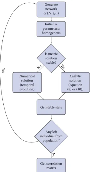
In conclusion, the variability within one same family of networks G N, μ brings about individual differences concerning variables which entail particular patterns or

structures of the correlation matrix (28), with no explicit constrains on parameters, but considering them as homoge-neous both along variables and individuals (see Figure 7).

R N, μ = f G N, μ 28

From Figure 8, we conclude that the positive manifold, that is, positive correlations, Rij> 0, can come out regardless

of the topology, as long as μ of the network is properly set. Thus, connectivity by itself allows positive interactions, regardless of the structure and independently of further con-strains on dynamic parameters. However, the structure of the correlation matrix indeed relies on the topology: Erdös-Rényi network’s correlation histogram displays a narrow symmet-ric peak which captures the homogeneity of the topology, that is, all nodes being equivalent. The distribution which comes out when considering this topology and identical parameters for all nodes is equivalent to the one obtained by [36] in the case of a complete network and heterogeneity in parameters. On the contrary, heterogeneous network’s correlation histogram follows a much wider asymmetric

Generate network G (N, {𝜇}) Initialize parameters: homogenous Is metric solution stable? Numerical solution (temporal evolution) Analytic solution (equation (8) or (10))

Get stable state

Any left individual from population? Get correlation matrix No Yes No Ye s

Figure 7: Flowchart to generate correlation matrix of variables out of a population of individuals.

distribution, with a longer tail for larger values. This behav-iour captures the presence of few hubs, which leads to non-trivial correlation structures, as we will see in Section 5.2. Finally, the Newman modular network presents two charac-teristic peaks corresponding to intracluster, that is, within the same cluster, and intercluster, that is, between different clus-ters, correlations. As k_in increases, both peaks become undistinguishable and the pattern more closely resembles an Erdös-Rényi network. For large k_in , intercluster correla-tions tend to 0 value.

So far, in addition to considering a homogeneous config-uration of parameters, we have constrained ourselves to solutions within the regime where metric stable solution is stable. Nevertheless, we expect richer phenomena when nei-ther of the two restrictions exists. If we allow K parameter to be a random variable distributed among variables following a noncorrelated normal distribution, N μK, σK , increasing

values of σK lead to lower values of Rij , the average

cor-relation between variables.

Figure 9 captures not only the positive manifold but also the effect of network topology on the correlations. Rij is

indeed modulated by the characteristic parameter of the network, μ . For Erdös-Rényi and heterogeneous networks,

Rij peaks around the transition between metric and optimal

stable states, with a profile shaped by the network topology. The average correlation increases as connectivity does so, until nodes are recurrently being absorbed by the optimal state and, consequently, Rij is scaled down. Namely,

Erdös-Rényi network peaks around pC, that is, when stability

changes landscape. As p increases, more and more variables reach the optimal value and become independent from others. The impact of more variability in K parameter across variables is the decrease in the correlations, and the peak

0 100 200 300 400 500 Co u n ts 0.0 0.1 0.2 0.3 0.4 0.5 0.6 0.7 0.8 −0.1 Rij (i ⇍ j) (a) 0 500 1000 1500 2000 2500 3000 Co u n ts 0.0 0.1 0.2 0.3 0.4 0.5 0.6 0.7 0.8 −0.1 Rij (i ⇍ j) (b) 0 1000 2000 3000 4000 5000 6000 7000 8000 C o un ts 0.0 0.1 0.2 0.3 0.4 0.5 0.6 0.7 0.8 −0.1 Rij (i ⇍ j) (c)

Figure 8: Histogram of the correlation between variables, R_ij, for 3 distinct network topologies: Erdös-Rényi of size N = 50 and edge probability p = 0 4 (a), heterogeneous network of size N = 200 and degree distribution exponent α = 2 9 (b), and Newman modular of size

N = 256, k_in = 15 and k_total = 16 (c). The histogram captures the effect of G N, μ on R N, μ . Correlation matrix is computed from analytic metric stable state (8) of 5000 generated individuals. The distribution of correlations between variables connected as an ER network is peaked at a certain value, whereas assuming a heterogeneous network leads to a much broader spectrum of correlation values. The Newman modular network brings about two clear peaks, corresponding to intracluster and intercluster correlations. Parameters of the model are set for all nodes to C = 5 and K = 1 for all networks, r = 1 and w = 0 03 for Erdös-Rényi network, r = 0 5 and w = 0 025 for heterogeneous network, and r = 0 05 and w = 0 015 for Newman modular network.

shifting towards lower values of p, since stability condition (21) is more likely to be broken. The peak generated by a heterogeneous network is more diffuse, owing to a wider distribution of the spectra. Moreover, the effect of increasing the variability in K has a stronger attenuation effect. On the contrary, the absence of a peak coming out from the

Newman modular network is explained in Section 4.3. Nevertheless, a clear pattern emerges if we split intracluster from intercluster mean correlations. While intracluster correlations increase as k_in does so, intercluster correlations decrease. However, the total mean correlation remains unchanged, as long as condition (21) is true.

0.00 0.05 0.10 0.15 0.20 0.25 0.30 0.35 〈Rij 〉 (i⇍j ) 0.2 0.3 0.4 0.5 0.6 0.7 0.8 0.9 0.1 p 𝜎_k= 0.0 𝜎_k= 0.1 𝜎_k= 0.2 𝜎_k= 0.3 𝜎_k= 0.4 𝜎_k= 0.5 (a) 𝜎_k= 0.0 𝜎_k= 0.1 𝜎_k= 0.2 𝜎_k= 0.3 𝜎_k= 0.4 𝜎_k= 0.5 0.00 0.05 0.10 0.15 0.20 0.25 0.30 〈Rij 〉 (i⇍j ) 2.1 2.2 2.3 2.4 2.5 2.6 2.7 2.8 2.9 3.0 2.0 𝛼 (b) 0.00 0.02 0.04 0.06 0.08 〈Rij 〉 (i⇍j ) 2 3 4 5 6 7 8 9 10 11 12 13 14 15 1 〈kin〉 𝜎_k= 0.0 𝜎_k= 0.1 𝜎_k= 0.2 𝜎_k= 0.3 𝜎_k= 0.4 𝜎_k= 0.5 (c)

Figure 9: For model A, defined in (3), the average correlation between variables, Rij, is plotted as a function of the characteristic network

parameter, μ , for 3 network topologies: Erdös-Rényi of size N = 50 (a), heterogeneous network of size N = 200 (b), and Newman modular of size N = 256 and ktotal = 16, where intracluster (dimmer upper) and intercluster (solid bottom) correlations are held separately (c). The

distribution of each value is captured by a boxplot computed from 50 independent realizations. Six different values of σK account for the

variability of K parameter. AsσKincreases, Rij is scaled down, being the effect much larger in heterogeneous networks. In the case of ER

network, Rij grows with increasing p until metric state eventually becomes unstable, and nodes are gradually absorbed by optimal state.

Larger dispersion on K shifts the peak towards lower values of p. Conversely, for a heterogenous network, an increase onα exponent leads to more stability of metric state, although stable conditions are more fragile. Larger dispersion on K shifts the peak towards much lower values ofα. Finally, in the case of Newman modular network, stability conditions of metric state, (21), are always true for these parameters and hence the absence of the peak. For a better understanding of change of stability landscape, see Figure 6. The parameters of the model are set as Figure 8.

For model B, Rij continuously increases as connectivity

does so, until divergence conditions are met, and solutions do not longer exist.

5.2. From Correlation Matrix to Statistical Models. When it comes to describing variability among observed, correlated variables, a bunch of statistical models comes along, aiming to approximate and understand reality. Factor analysis is a statistical method developed and widely used in psychomet-rics [64, 67–69], inter alia. Observed variables are described as linear combinations of unobserved latent variables or factors, plus individual error terms, such that covariance or correlation matrix may be explained by fewer latent variables. Historically, the most widely held theories of cognition and intelligence are built upon factor analysis raising from large batteries of conducted psychometric tests. There is still no agreement on the proper model and the underlying pro-cess which bring about the observed outcome. We list the models stood for the most outstanding theories: one factor models, multifactorial models, hierarchical models, and other more complex structural models [70].

Section 5.1 evinces that connectivity structure between variables, mapped on a particular network topology, gives rise to different correlation matrices, even no explicit con-strains on correlations between parameters are imposed. We show that certain factor models can be explained by a mutualistic dynamical model running on a particular network of variables.

In order to avoid subjective criteria when deciding the number of factors, several methods have been devel-oped: Horn’s parallel analysis, Velicer’s map test, Kaiser criteria, Cattell scree plot, or variance explained criteria [71–74]. We proceed to compute the scree plot so as to obtain the number of main principal components and hence potential latent factors. Thereupon, the statisti-cal significance of the factor model is assessed by means of the p value, which enables us to explore the effect of changing the parameter which best characterizes the network, μ .

In Figure 10, we have selected one specific network for each topology, given by the value of the characteristic parameter. The choice is such that solution is given by the metric stable state (8).

The number of retained components, or factors, can be obtained according to different criteria. We look at values which are much larger than 1 and display rather straight angles with the successive values.

With these criteria and from Figure 10, we hypothesize that the correlation matrix of variables which are connected following an Erdös-Rényi network is well described by a 1-factor model. In the case where their connectivity struc-ture is better capstruc-tured by a Newman modular network with

n clusters, then an n-factor model cannot be rejected.

Con-versely, considering a heterogeneous network, a factorial model is no longer proposed, as eigenvalues are not clearly separated according to former criteria, but rather they follow a smooth decreasing curve. Alternatively, a statistical model which accounts for hierarchy between variables or more complex structural modelling and path analysis may be more

realistic. However, this latter analysis is out of the scope of this paper.

For the cases of Erdös-Rényi and Newman modular networks with 4 clusters, we show that a 1-factor model and a 4-factor model, respectively, can be accurate models to obtain results. To do so, we compute the p value of such models for different numbers of retained factors. p value in this case is testing the hypothesis that the model fits the results perfectly, and hence we seek values > 0.05.

In the case of an Erdös-Rényi network, p value≈ 1 ≫ 0.05 for n_factors≥ 1, and hence a 1-factor model is highly likely. Similarly, in the case of a Newman modular network with

n = 4, p value > 0.05 only when nfactors≥ 4, as suggested (see Figure 11).

Once we have figured out the number of factors with respect to each network, we explore the effect of connectivity on the reinforcement of the statistical models, by looking at the explained variance of the most important components:

var R i=

λi

〠_kλk

29

We make use of (29), which gives the proportion of explained variance ofR correlation matrix for each principal component of PCA. Although PCA and FCA are not equiv-alent statistical models [75, 76], after having sustained the

100 101 102 𝜆 (R ) 4 6 8 10 12 14 2 Number of components Heterogeneous (𝛼 = 2.9) Erdös-Rényi (p = 0.4) Newman modular (〈k_in〉 = 15)

Figure 10: Scree plot, in logarithmic vertical scale, calculated from the correlation matrix, R, for 3 network topologies: Erdös-Rényi (triangular orange markers), heterogeneous (circular blue markers), and Newman modular (squared green markers) networks, with parameters as in Figure 9. A scree plot shows the value of eigenvalues, λ R , in descending order, as components (principal orthogonal directions) are gradually being included (up to the number of variables).λ = 1 is labelled in red, as a possible selection criterion for the number of components or factors. Other used criteria: λ R much larger than the others and describing rather straight angles with successive values. 1-factor model and 4-factor model may be suitable for ER and Newman modular networks, respectively, whereas a more complex model is needed for heterogeneous network.

validity of a factor model, the former approach is acceptable in order to justify the suitability of the number of factors or components considered.

Figure 12 confirms the assumptions underlying the models for both networks: in the case of an Erdös-Rényi network, the first eigenvalue increases as connectivity,

characterized by p, does so, and hence a 1-factor model is being reinforced. Similarly, in the case of a Newman modular network, besides the first eigenvalue, which is always large, second to fourth eigenvalues increase as modularity, charac-terized by k_in , does so, in contrast to eigenvalues on further positions, which remain unchanged or smaller.

0.20 0.25 0.30 0.35 0.40 0.45 p 0 5 10 15 20 25 30 %va r ( R ) 𝜆1/Σk = Nk = 1𝜆k k = N k = 1 𝜆2/Σ 𝜆k k = N k = 1 𝜆3/Σ 𝜆k k = N k = 1 𝜆4/Σ 𝜆k k = N k = 1 𝜆5/Σ 𝜆k (a) 6 8 10 12 14 0.6 0.8 1.0 1.2 1.4 %va r ( R ) 〈kin〉 𝜆1/Σ k = N k = 1𝜆k k = N k = 1 𝜆2/Σ 𝜆k k = N k = 1 𝜆3/Σ 𝜆k k = N k = 1 𝜆4/Σ 𝜆k k = N k = 1 𝜆5/Σ 𝜆k (b)

Figure 12: Percentage of the total explained variance of correlation matrix %var R , (29), for each of the first five components λ R as a function of the edge probability, p, for an Erdös-Rényi of size N = 50 (a), and intracluster degree, kin, for a Newman modular network of size N = 256 and k_total = 16 (b). Both networks enable a factor model as a good descriptor of the outcome. Selected significant number of components are highlighted in orange and green colors, for ER and Newman modular networks, respectively. As nodes become more connected and communities more delimited, factor model moves from mirroring a noisy identity matrix to be a clear indicator of the correlation structure. First component (circular orange marker) increases as p does so, strengthening the validity of a 1-factor model (a), while second to fourth components (circular, starry, and triangular green markers) increase as k_in does so. Hence, an increase in modularity reinforces the validity of a 4-factor model (b). Parameters are set as in Figure 6, constraining the values to lay within the metric stable state regime.

0.0 0.2 0.4 0.6 0.8 1.0 p val u e 2 3 4 5 1 nfactors (a) 0.0 0.2 0.4 0.6 0.8 1.0 p val u e 2 3 4 5 1 nfactors (b)

Figure 11: P-values obtained for a factorial model with a number of factors ranging 1 to 5, for 2 network topologies: Erdös-Rényi of size

N = 50 and p = 0 4 (a) and Newman modular of size N = 256, ktotal = 16, and kin = 15 (b) networks, with parameters as in Figure 9. p value = 0.05 is labelled in orange, as threshold for not rejecting the model.

We are mostly interested in the qualitative results. Differ-ent network sizes and dynamic parameters lead to differDiffer-ent values for the eigenvalues and variances, while showing the same patterns [77].

We have provided an alternative explanation of data being well described by different factor models. However, alternative statistical models ought to be considered in the case of Newman modular network to obtain more pre-cise insights, namely, bifactor and second-order factor models, which are the most popular factor models in the intelligence literature.

Covariance matrix can be analytically computed in the case of a complete network and a heterogeneous parameter landscape, K~N μK, σK (Appendix B).

6. Conclusions

Despite mainstream approaches to cognition and intelligence research are built on static and statistics-based models, we explore the emerging dynamical systems perspective putting a greater emphasis on the role of the network topology underlying the relationships between cognitive processes.

We go through a couple of models of distinct cognitive phenomena and yet find the conditions for them to be mathematically equivalent. Both models meet the require-ments set out by empirical observations and established theories regarding the corresponding cognitive phenomena to which they aim to provide an explanation, namely, the positive manifold and the suitability of several statistical models. Furthermore, the applied mathematical formulation may well enlight models of many real mutualistic systems, other than cognitive.

The topology of the network defined by the dynamical influence between processes indeed underlays further analy-sis of the results. Wefind the principal attractor of the system to be the exact definition of Katz-Bonacich centrality, a measure of a node importance which can also be understood as a nonconservative biased random walk along a network. We propose that heterogeneities in the dynamical parameters can be absorbed by a rescaling of the adjacency matrix weights and hence leading to the same result.

Individuals may differ not only in the genetic-environmental markers captured by the parameters of the model, but also in the connectivity structure between brain regions, either structural or functional. Two individuals might achieve the same performance through different neuronal routes or architectures and cognitive strategies when solving cognitive tasks. Certain common brain struc-tures and functional pathways may be more likely to be involved in intelligence than others. However, despite of the heterogeneity between subjects, cognitive outcomes may result similar [14]. For instance, as Newman modular network increases its modularity, the corresponding corre-lation matrix becomes more and more likely to be well described by a factorial model with as many factors as communities it has. However, whereas the inner structure gradually changes, the average result of its stable state remains unchanged.

The connectivity structure between cognitive processes is not known but yet it is not any. We show that network topology by its own leads to different plausible statistical models. Regardless of the network considered, it is always possible to set a parameter configuration such that the pos-itive manifold results from the dynamical model. However, the correlation structure is determined by the network topology. Complete and Erdös-Rényi networks are con-strained to bring about a one-factor model, more clearly defined as connectivity increases. The Newman modular network enables higher-order factor models, depending on the number of defined communities. Latent factors turn to be more distinguishable as modules grow to be more isolated. Conversely, heterogeneous networks lead to richer correlation structures, which may be better described by more complex statistical models.

In the present article, we exploit the interplay between the dynamics and the underlying network topology to model cognitive abilities, and we conclude that both of the two are relevant. Although scholars are not yet sure of the relation-ship between cognitive processes and of the nature of intelligence, we can shed a bit of light by proposing an alternative framework which captures the real meaning of “process” and “relationship”: a dynamic complex network framework to model cognition.

This work is an open door to further research: we show that different network topologies lead to different correlation structures. Still, richer topologies can be considered and may bring about other interesting and eventually more realistic structures. We have restricted ourselves to static networks, though the more general definition of a network is not time constrained. What if the network which captures the connec-tion between cognitive processes or brain modules was time dependent? What if cognitive processes could be modelled as a multilayer network, from generalists to specialists layers? Moreover, when looking only at the attractors of the system, we are missing the temporal evolution of such processes and its real causality. Therefore, are these models able to explain evolving properties of the considered variables? We finally highlight that there exist several limitations in models based on ecologic systems, as exhaustively studied in pop-ulation dynamics research, namely, inconsistent results coming from unbounded models and discrepancy with the behaviour of some real systems [78–81]. Hence, alterna-tive mathematical models which overcome some of these problems shall be investigated.

Appendix

A. Average and Variance of Stable Solution for a

Complete and an Erdös-Rényi Network

We define homogeneous configuration as follows:

Ki≡ K ∀i,

ri≡ r ∀i,

Wij≡ w ∀ i, j

In this case, metric stable solution (10) for a complete network is straighforward: xi= 0⇒ 1 − x∗− N − 1 wx∗ K = 0⇒x ∗ = K 1 − w N − 1  ∀i A 2

In the case of a complete network, as solutions are exactly the same for all nodes, the variance of stable state is null.

For an Erdös-Rényi network, we compute the average of metric stable state:

x∗= 1

N〠_i 〠_j I − W

T −1

ijKj A 3

Using (18) and considering W is a symmetric matrix, though the expression is equivalent,

I − WT −1 ij= I − W −1 ij = δij+ Wij+ 〠 k WikWkj + 〠 k 〠 l WikWklWlj+ ⋯ A 4

Taking the average on (A.4), 1 N〠_i 〠_j I − W T −1 ijKj = K 1 N〠_i 〠_j I − W T −1 ij = K 1 N〠_i 〠_j δij+ Wij+ 〠_k WikWkj + 〠 k 〠 l WikWklWlk+ ⋯ = K 1 N〠_i 〠_j δij+ 1 N〠_i 〠_j Wij+ 1 N〠_i 〠_j 〠_k WikWkj + 1 N〠_i 〠_j 〠_k 〠_l WikWklWlj+ ⋯ A 5 We proceed to calculate each term of the average:

1

N〠_i 〠_j δij= 1, A 6

1

N〠_i 〠_j Wij= wk, A 7

where k≡ 1/N ∑ikiis the mean degree of a node.

Second and following terms account for the average number of m next-nearest neighbours, denoted with zm.

The general expression for any network is given by [82]

zm= z₂ z₁ m−1 z₁, A 8 where z₁= k.

In the case of an Erdös-Rényi network following a Poisson distribution, we get

zm= km ∀m A 9

Using (A.6), (A.7), and (A.9),

x∗_ER= 1 N〠_i 〠_j I − W T −1 ijKj = 1 + wk + w2k2+ w3k3+ ⋯ = K 1 − wk ∀i A 10

We point out the fact that a Poisson distribution is not always a good model for an Erdös-Rényi network, and hence (A.10) is considered an approximation for x∗_ER.

The variance of x∗_i, var x∗_{i ER}, is a rather difficult compu-tation, and therefore we explore the behaviour at the second order of w, ~O w2 _:

cov x∗i, x∗j ≡ cov = xixj − xi xi , A 11

where · corresponds to the average of the ensemble. The second term, xi , is already known (A.10), as it is

given byx∗in the thermodynamic limit. Using (10), thefirst term can be expanded as

xixj K2 = 〠 q δjq+ w〠 q Ajq+ w2〠 q 〠 k′ Ajk′Ak′q + w〠 q δjq〠 p Aip+ +w2〠 q Ajq〠 p Aip + w2〠 q δjq〠 p 〠 k AikAkp+ O w3 A 12

Using (A.8) and splitting the cases i = j and i ≠ j,

cov x∗i, x∗j

ER≈ O w

3 _{∀i, j,}

var x∗_{i ER}≈ k2w2var k + O w3  ∀i

A 13

Therefore, in order to obtain further information of the structure of the covariance and correlation matrices, we ought to compute higher orders on w.

Nevertheless, we have proved that the covariance matrix is made out of two different values: the diagonal and

off-diagonal elements. The covariance matrix,Σ, can be written as follows: Σ = a b ⋯ b b a ⋯ b ⋯ ⋯ ⋯ ⋯ b b ⋯ a A 14

A requirement for a covariance matrix,Σ, to be explained by a one-factor model is that the spectral gapλ₁− λ₂is large enough, that is,λ₁≫ λ₂:

λ1= a + N − 1 b,

λ2⋯N= a − b

A 15

Hence,λ₁− λ₂= Nb, which increases as the number of variables or b do so and enables a one-factor model to fit the results.

B. Covariance Matrix for a Complete

Network and Heterogeneous

Parameter Configuration

Although the solution when connectivity structure is captured by a complete network is trivial, we can go a step further when taking into account variability in the dynamic parameters, as it was similarly done in the appendix of [36].

Let us consider K parameter taken from a normal uncorre-lated distribution, Ki~N μK, σK : KiKj = Ki Kj = μ2K, σ2 K+ Ki 2= σ2K+ μ2K, if i ≠ j B 1

If we separate xixj according to the contribution

regarding K parameter, xixj = a2 KiKj + ab Ki〠 q≠j Kq + ab 〠 p≠i KpKj + b2 〠 q≠j Kq〠 p≠i Kp , B 2 where a≡ 1 − N − 2 w / 1 − N − 2 w − N − 1 w2 _and b≡ w/ 1 − N − 2 w − N − 1 w2 _.

Using (A.11), covariance matrix can finally be written as follows:

cov ≡

var x cov x ⋯ cov cov x var x ⋯ cov x

⋯ ⋯ ⋯ ⋯

cov x cov x ⋯ var x

, B 3 where and vov ≡ K 2 _−w2 _{N− 2}2_{+ 2w N − 2 N − 2 − 1 + σ}2 Kw2 N− 2 1 + w2 1 − N − 1 w2 B 5

From (B.3), it turns out that a 1-factor model is indeed valid for the description of the covariance matrix. In cases where cov x ~ var x , then adequacy decreases. The partic-ular case cov x = var x is achieved when w = 1/ N − 3 . However, such condition is never reached:

w > 1

N− 1 B 6

As seen from (12), stable state diverges when

w > 1/ N− 1 .

C. Stability Conditions

To obtain the stability conditions of optimalfixed point (7), we expand (3) around thisfixed point xi≡ x C i+ ϵi:

ϵi= ri C + ϵi 1 − C + ϵi C 1 − C + ϵi − Ki/ri〠jWji C + ϵi Ki C 1

If we linearize (C.1) keeping only terms ~O ϵi , we

obtain ϵi≈ −ϵi ri 1 − C Ki + C〠 j Wji ≡ −βiϵi C 2 var x ≡ K 2 _−w2 _{N− 2}2_{+ 2w N − 2 − 1 + σ}2 K w2 N− 2 + 1 − N − 3 w 1 + w2 1 − N − 1 w2 B 4

On the other hand, to obtain the stability conditions of metricfixed point (8), we expand (3) around this fixed point

xi≡ x Wd i+ ϵi: ϵi≈ −x Wd i 1 − x W_{d i} C ϵi− Ki ri 〠 j Wjiϵj C 3

Equation (C.3) can be written in matrix forms as (22). We can derive a threshold for the stability condition using the Perron-Frobenius theorem, (23), applied to (22) which enables us to write

λmax S < −x Wd i 1 − x W_{d i} C 1 − K_i r_i〠_j Wji max < 0 C 4 Looking into the extreme conditions of (C.4), we conclude 1 − Ki r_i〠_j Wji > 0⇒ Ki r_i 〠_j Wji max ≡ 〠 j Wd ij max < 1 C 5

Data Availability

The data used to support the findings of this study are available from the corresponding author upon request.

Conflicts of Interest

The authors declare that there is no conflict of interests regarding the publication of this paper.

Acknowledgments

The authors acknowledge the financial support from MINECO under Project no. FIS2012-38266-C02-02 and no. FIS2015-71582-C2-2-P (MINECO/FEDER) and Generalitat de Catalunya under the Grant no. 2014SGR608. Gemma Rosell-Tarragó acknowledges MECD under Grant no. FPU15/03053. The authors wish to express their gratitude to Joan Guàrdia for his revision and comments on the work.

References

[1] E. M. Tucker-Drob, “Differentiation of cognitive abilities across the life span,” Developmental Psychology, vol. 45, no. 4, pp. 1097–1118, 2009.

[2] R. Kanfer,“Motivation and individual differences in learning: an integration of developmental, differential and cognitive perspectives,” Learning and Individual Differences, vol. 2, no. 2, pp. 221–239, 1990.

[3] D. H. Jonassen and B. L. Grabowski, Handbook of Indi-vidual Differences, Learning, and Instruction, L. Erlbaum Associates, 1993.

[4] R. J. Sternberg and L.-F. Zhang, Perspectives on Thinking, Learning, and Cognitive Styles, Lawrence Erlbaum Associ-ates, 2001.

[5] U. Neisser, G. Boodoo, T. J. Bouchard Jr. et al.,“Intelligence: knowns and unknowns,” American Psychologist, vol. 51, no. 2, pp. 77–101, 1996.

[6] E. E. Smith and S. M. Kosslyn, Cognitive Psychology: Mind and Brain, Prentice Hall, 2009.

[7] H. J. Eysenck, “The concept of “intelligence”: useful or useless?,” Intelligence, vol. 12, no. 1, pp. 1–16, 1988.

[8] R. J. Herrnstein and C. A. Murray, The Bell Curve: Intelligence and Class Structure in American Life, Simon & Schuster, 1996. [9] H. Rindermann,“The g-factor of international cognitive ability comparisons: the homogeneity of results in PISA, TIMSS, PIRLS and IQ-tests across nations,” European Journal of Personality, vol. 21, no. 5, pp. 667–706, 2007.

[10] Z. Stein and K. Heikkinen, “Models, metrics, and measure-ment in developmeasure-mental psychology,” Integral Review, vol. 5, no. 1, pp. 4–24, 2009.

[11] G. S. Lesser, G. Fifer, and D. H. Clark, “Mental abilities of children from different social-class and cultural groups,” Monographs of the Society for Research in Child Development, vol. 30, no. 4, pp. 1–115, 1965.

[12] H. Gardner, Frames of Mind, Basic Books, New York, NY, USA, 1983.

[13] L. Erlenmeyer-Kimling and L. F. Jarvik, “Genetics and

intelligence: a review,” Science, vol. 142, no. 3598, pp. 1477– 1479, 1963.

[14] I. J. Deary, L. Penke, and W. Johnson,“The neuroscience of human intelligence differences,” Nature Reviews Neuroscience, vol. 11, no. 3, pp. 201–211, 2010.

[15] J. R. Gray and P. M. Thompson,“Neurobiology of intelligence: science and ethics,” Nature Reviews Neuroscience, vol. 5, no. 6, pp. 471–482, 2004.

[16] M. G. Mattar and D. S. Bassett,“Brain network architecture: implications for human learning,” 2016, https://arxiv.org/ abs/1609.01790.

[17] J. D. Bransford, A. L. Brown, and R. R. Cocking, How People Learn, National Academy Press, Washington, DC, USA, 2000. [18] J. B. Carroll, Human Cognitive Abilities. A Survey of Factor-Analytic Studies, Cambridge University Press, Cambridge, UK, 1993.

[19] P. L. Ackerman,“Individual differences in skill learning: an integration of psychometric and information processing per-spectives,” Psychological Bulletin, vol. 102, no. 1, pp. 3–27, 1987. [20] S. B. Kaufman, M. R. Reynolds, X. Liu, A. S. Kaufman, and K. S. McGrew,“Are cognitive g and academic achievement g one and the same g? An exploration on the Woodcock– Johnson and Kaufman tests,” Intelligence, vol. 40, no. 2, pp. 123–138, 2012.

[21] J. L. Castejon, A. M. Perez, and R. Gilar,“Confirmatory factor analysis of Project Spectrum activities. A second-order g factor or multiple intelligences?,” Intelligence, vol. 38, no. 5, pp. 481– 496, 2010.

[22] D. Molenaar, C. V. Dolan, J. M. Wicherts, and H. L. J. van der Maas,“Modeling differentiation of cognitive abilities within the higher-order factor model using moderated factor analy-sis,” Intelligence, vol. 38, no. 6, pp. 611–624, 2010.

[23] W. Johnson, J. t. Nijenhuis, and T. J. Bouchard Jr.,“Still just 1 g: consistent results from five test batteries,” Intelligence, vol. 36, no. 1, pp. 81–95, 2008.

[24] P. L. Ackerman, M. E. Beier, and M. O. Boyle, “Working

memory and intelligence: the same or different constructs?,” Psychological Bulletin, vol. 131, no. 1, pp. 30–60, 2005.