High Performance Computing on
CRESCO infrastructure:
research activities and results 2016
Italian National Agency for New Technologies,
High Perfor research act Contribution Scientific E Acknowled (http://hdl.h Cover: Ame rmance Com tivities and r ns provided Editor: Miche gements: We handle.net/10 edeo Trolese, mputing on CR esults 2016 by a selectio ele Gusso, EN e wish to tha 0840/5791) to , ENEA, DT RESCO Infra on of users of NEA, DTE-I ank Gianclau o collect the E-ICT-PRA astructure: f the CRESC ICT-HPC, Br udio Ferro fo contribution , Frascati Re CO infrastruc rindisi Resea or providing ns and to buil esearch Centr cture arch Centre the Reporter ld the Volum re r system me
Contents
Foreword
5
M-TraCE: the development of a new tool in CRESCO-HPC environment for high
resolution elaboration of backward trajectories
L. Vitali, M. D'Isidoro, G. Cremona, E. Petralia, A. Piersanti, G. Righini
6
Atmospheric pollution trends simulated for the period 1990–2010 in Europe:
EURODELTA - Trends project
M. Adani, G. Briganti, A. Cappelletti, M. D'Isidoro, M. Mircea
10
The I/O benchmarking methodology of EoCoE project
S. Luehrs, A. Funel, M. Haefele, F. Ambrosino, G. Bracco, A. Colavincenzo, G.
Guarnieri, M. Gusso, G. Ponti
16
The effect of hydrostatic pressure on the structural and superconducting properties of A15
Nb3Sn
R. Loria, G. De Marzi
23
Organocatalytic Coupling of Bromo-Lactide with Cyclic Ethers and Carbonates
L. Cavallo, L. Caporaso, L. Falivene, R. Credendino
29
Ab initio formation energy of hydrogenated graphene oxides
F. Buonocore, N. Lisi
33
The role of plant phenology in stomatal ozone flux modelling
A. Anav, A. De Marco
40
Calibration of the high resolution regional earth system model (RegESM) over the
Med-CORDEX domain
M. V. Struglia, S. Calmanti, A. Carillo, A. Dell'Aquila, E. Lombardi, G. Sannino
43
A neural network for molecular dynamics simulations of hydrogenated amorphous silicon
M. Gusso, J. Behler
47
Inter-layer synchronization in non-identical multilayer networks
I. Sendina-Nadal, I. Leyva, R. Sevilla-Escoboza, R. Gutiérrez, J. M. Buldú, S. Boccaletti
52
FARO2.0 - A renewed gateway to ENEAGRID resources
Cloud infrastructure for scalability and high availability in business ICT applications
A. Mariano, F. Beone, A. Scalise
66
Analysis of diffraction pattern for cadmium sulfide nanocluster by using Debye scattering
equation
E. Burresi, M. Celino, L. Tapfer
72
Theory and modeling of energetic particle driven instabilities
S. Briguglio, G. Fogaccia, V. Fusco, G. Vlad, X. Wang, T. Wang
78
Neutron Transport analysis in DEMO in-vessel components
R. Villari, D. Flammini, F. Moro
86
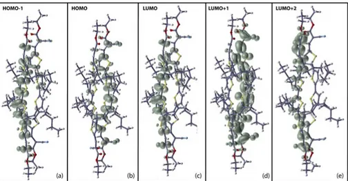
Electronic excitations in small oligothiophene molecules
F. Gala, G. Zollo
90
Monte Carlo simulations supporting safety studies of PWR’s and irradiation tests in
TAPIRO research reactor
P. Console Camprini, K. W. Burn
100
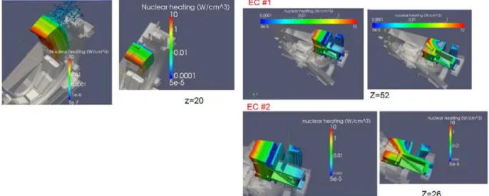
Nuclear responses in the ITER IVVS port cell
D. Flammini, F. Moro, R. Villari
105
Edge modeling with SOLEDGED2-EIRENE code in RFX-mod and TCV fusion devices
P. Innocente
109
Ab-initio study of the c-Si/a-Si:H interface for PV technology
S. Giusepponi, M. Celino, M. Gusso, U. Aeberhard, P. Czaja
113
Molecular dynamics of GeO2: Car-Parrinello simulations in the range 10-4000 K
G. Mancini, M. Celino, A. Di Cicco
117
Development of the new circulation forecast model for the Mediterranean Sea
G. Sannino, A. Carillo, A. Bargagli, E. Lombardi
122
Computational design and validation of a reconfigurable three-dimensional DNA
nanostructure
F. Iacovelli, M. Falconi
126
Calculation of correction factors for solid-state detectors in radiotherapy photon beams
M. Pimpinella, L. Silvi
133
An alternative use of prompt-Self Powered Neutron Detectors: spectral-deconvolution for
monitoring high-intensity neutron fluxes
L. Lepore, R. Remetti, A. Pietropaolo
141
Neutronic analyses in support of the WCLL DEMO design development
F. Moro, D. Flammini, R. Villari
149
Report on CFD simulations of LOVA (Loss of vacuum accident) with ANSYS CFX 17.0
EUROfusion engineering grant safety analysis
F. Tieri
154
Quantitative in situ gamma spectrometry in contaminated soil
M. Altavilla
158
Influence of mass media in the Naming Game
F. Palombi, S. Ferriani, S. Toti
161
Forces exerted by a solitary wave on horizontal cylinder
L. Gurnari, P. Filianoti
167
High pressure premixed CH4/H2-Air flames
D. Cecere, E. Giacomazzi, N. Arcidiacono, F. R. Picchia
172
Definition of a figure of merit for the optimization of ENEA NAI device
R. Remetti, G. Gandolfo, L. Lepore, N. Cherubini
179
Structure of metal oxide nanoclusters from ab-initio computation
R. Grena
185
Smagorinsky dynamic model for large-eddy simulation of turbulence
G. Rossi, D. Cecere, E. Giacomazzi, N. M. S. Arcidiacono, F. R. Picchia, B. Favini
189
Characterization of MCL1 inhibition via Fast Switching Double annihilation technology
on the CRESCO3 cluster
P. Procacci
195
DPPC biomembrane solubilization by Triton TX-100: a computational study
A. Pizzirusso, A. De Nicola, G. J. A. Sevink, A. Correa, M. Cascella, T. Kawakatsu, M.
Rocco, Y. Zhao, M. Celino, G. Milano
202
Variant discovery for Triticum durum variety identification
Materials for energy in the framework of the european center of excellence EoCoE
M. Celino, S. Giusepponi, M. Gusso, U. Aeberhard, A. Walker, S. Islam, D. Borgis, X.
Blase, M. Salanne, M. Burbano, T. Deutsch, L. Genovese, M. Athenes, M. Levesque, P.
Pochet
216
Cavity design for a cyclotron auto-resonance maser (CARM) radiation at high frequency
S. Ceccuzzi, G. Dattoli, E. Di Palma, G. L. Ravera, E. Sabia, I. Spassovsky
222
First principle studies of materials for energy conversion and storage
M. Pavone, A. B. Munoz-Garcia, E. Schiavo
227
Role of the Sub-surface Vacancy in the amino-acids adsorption on the (101) Anatase TiO2
surface: A first-principles study
L. Maggi, F. Gala, G. Zollo
233
LES of heat transfer in an asymmetric rib-roughened duct: influence of rotation
D. Borello, A. Salvagni, F. Rispoli
238
SOLEDGE2D-EIRENE simulations of the reference scenario of the M15-20 JET
experiment
Foreword
During the year 2016, CRESCO high performance computing clusters have provided about 43 million
hours of “core” computing time, at a high availability rate, to more than one hundred users, supporting
ENEA research and development activities in many relevant scientific and technological domains. In
the framework of joint programs with ENEA researchers and technologists, computational services
have been provided also to academic and industrial communities.
This report, the eighth of a series started in 2008, is a collection of 45 papers illustrating the main
results obtained during 2016 using CRESCO/ENEAGRID HPC facilities. The significant number of
contributions testifies the importance of the interest for HPC facilities in ENEA research community.
The topics cover various fields of research, such as materials science, efficient combustion, climate
research, nuclear technology, plasma physics, biotechnology, aerospace, complex systems physics,
renewable energies, environmental issues, HPC technology. The report shows the wide spectrum of
applications of high performance computing, which has become an all-round enabling technology for
science and engineering.
Since 2008, the main ENEA computational resources is located near Naples, in Portici Research
Centre. This is a result of the CRESCO Project (Computational Centre for Research on Complex
Systems), co-funded, in the framework of the 2001-2006 PON (European Regional Development
Funds Program), by the Italian Ministry of Education, University and Research (MIUR).
The Project CRESCO provided the resources to set up the first HPC x86_64 Linux cluster in ENEA,
achieving a computing power relevant on Italian national scale (it ranked 126 in the HPC Top 500 June
2008 world list, with 17.1 Tflops and 2504 cpu cores). It was later decided to keep CRESCO as the
signature name for all the Linux clusters in the ENEAGRID infrastructure, which integrates all ENEA
scientific computing systems, and is currently distributed in six Italian sites. CRESCO computing
resources were later upgraded in the framework of PON 2007-2013 with the project TEDAT and the
cluster CRESCO4, 100 Tflops computing power. In 2016 the ENEAGRID computational resources
consist of about 8500 computing cores (in production) and a raw data storage of about 1400 TB.
The success and the quality of the results produced by CRESCO stress the role that HPC facilities can
play in supporting science and technology for all ENEA activities, national and international
collaborations, and the ongoing renewal of the infrastructure provides the basis for an upkeep of this
role in the forthcoming years.
In this context, 2015 is also marked by the signature of an agreement between ENEA and CINECA, the
main HPC institution in Italy, to promote joint activities and projects. In this framework, CINECA and
ENEA participated successfully to a selection launched by EUROfusion, the European Consortium for
the Development of Fusion Energy, for the procurement of a several PFlops HPC system, beating the
competition of 7 other institutions. The new system MARCONI-FUSION started operation in July
2016 at 1 Pflops computation power level which has been increased to 5 Pflops in the summer of 2017.
The ENEA-CINECA agreement is a promising basis for the future development of ENEA HPC
resources in the coming years. A new CRESCO6 cluster of 0.7 Pflops is planned to be installed before
the end of the current year, 2017.
Dipartimento Tecnologie Energetiche,
Divisione per lo Sviluppo Sistemi per l'Informatica e l'ICT - CRESCO Team
M-T
RA
CE:
THE DEVELOPMENT OF A NEW TOOL
IN CRESCO
-
HPC ENVIRONMENT FOR
HIGH RESOLUTION ELABORATION OF BACKWARD TRAJECTORIES
Lina Vitali
1*, Massimo D’Isidoro
1, Giuseppe Cremona
1, Ettore Petralia
1, Antonio Piersanti
1and Gaia Righini
11ENEA SSPT-MET-INAT, Via Martiri di Monte Sole 4, 40129, Bologna, Italy1
ABSTRACT. This work describes a new tool for the calculation and the statistical
elaboration of backward trajectories. In order to take advantage of the high resolution meteorological database of the Italian national air quality model MINNI, stored in CRESCO-HPC environment, a dedicated set of procedures was implemented, in same environment, under the name of M-TraCE, MINNI module for Trajectories Calculation and statistical Elaboration.
1 Introduction
Backward trajectory analysis is commonly used in a variety of atmospheric analyses [1]. In particular it is meaningful interpreting air composition measurements with respect to air mass origin and path through the atmosphere [2]. Backward trajectories are helpful for the interpretation of a single local event [3, 4], or can be processed through statistical analysis in order to provide information on the main directions of air masses fluxes and so on the region of influence of a site of interest [5]. Inter-comparison studies [6, 7] between different back trajectory models have shown that model performances are mainly determined by the quality and the spatial and temporal resolution of the underlying meteorological dataset, especially when complex terrain is involved [8, 9].
Here, the development of a new tool for backward trajectory analysis on the Italian territory is presented. Being the Italian peninsula characterized by complex orography, the usage of high resolution fields is mandatory to adequately describe the meteorological features. Italian National AMS-MINNI [10] meteorological database, at 4 km spatial resolution, has been used for this purpose. Furthermore, in some cases, additional ad-hoc meteorological simulations have been carried out at higher resolution (1 km) in order to better describe local meteorological features nearby the site of interest.
2 Methodology
2.1 Implemented procedures
M-TraCE is a package of procedures for high resolution computation and statistical elaboration of backward trajectories. M-TraCE is grouped into three main modules:
~ CORE: the core of the code, written in NCL [11], which calculates a single trajectory arriving at the site of interest at a selected time
~ LOOP: the procedure which allows looping to automatically calculate multiple trajectories ~ STAT: the procedure for the statistical processing of a sample of trajectories.
*
The core of the code is inspired by the HYSPLIT [12] model. In particular the method of Petterssen [13], a discrete numerical integration scheme based on simple Euler steps, is used to calculate air masses movements.
The result is the three-dimensional pathway of the trajectory provided both as graphical display and text file (Fig. 1).
Fig.1: The three-dimensional pathway of the trajectory: graphical display (top) and text file (bottom).
When the LOOP procedure is selected, the core code is recursively run on multiple cases; the output is a broad set of trajectories suitable for statistical analysis through the STAT procedure. In particular the following set of statistical parameters, are processed at the same horizontal resolution of the ingested wind field:
~ trajectories transits number in order to identify the main circulation patterns (e.g., Fig. 2); ~ the residence time (time spent by air mass in each spatial cell), for assessing regions of influence; ~ the average transport time, for the delimitation of the maximum extension of the area of spatial
representativeness, according to [14];
~ information on the height of air masses falling into each cell (minimum, maximum and average).
2.2 MINNI meteorological database
Wind fields for M-TraCE trajectories calculation are supplied by AMS-MINNI meteorological database, produced and stored in CRESCO-HPC environment, using the prognostic non-hydrostatic meteorological model RAMS [15].
RAMS is highly customizable for a wide range of applications, specifically for different spatial scales. In particular a multiple grid nesting scheme allows for the solution of model equations simultaneously on any number of interacting computational meshes of differing spatial resolution. The highest resolution meshes are used to model small scale atmospheric features, whereas coarse meshes are used to simulate large scale atmospheric systems that interact with the smaller scale ones. These features make RAMS suitable for high-resolution simulations, especially in case of complex terrain environments.
A comprehensive validation of the calculated AMS-MINNI meteorological fields is systematically carried out through the comparison with independent observations [16].
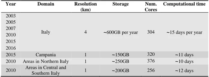
Actually, M-TraCE relies on an official, high spatial and time resolution, validated database and its development and usage represent a new further valorisation of the MINNI products availability. Table 1 summarizes the features of AMS-MINNI meteorological database, stored in CRESCO-HPC environment, including typical computation resources employed for meteorological simulation at different spatial resolutions.
Table 1: Features of the AMS-MINNI meteorological database and hardware usage.
Year Domain Resolution
(km)
Storage Num.
Cores
Computational time
2003
Italy 4
~
600GB per year 304~
15 days per year 2005 2007 2010 2015 2016 2015 Campania 1~
150GB 320~
11 days2010 Areas in Northern Italy 1
~
250GB 376~
10 days 2010 Areas in Central andSouthern Italy 1
~
200GB 256~
12 days3 Applications and current works
A preliminary version of M-TraCE, i.e. the module for single backward trajectory computation, was used to interpret in situ vertical profiles of aerosol physical properties [9].
The
complete and upgraded version of the tool, including routines for statistical elaboration, was applied for the first time to the sites of the Italian Network of Special Purpose Monitoring Stations, designed and maintained by the Italian Ministry of the Environment, Land and Sea [17].Recently M-TraCE has been used to support source apportionment assessment in the neighbourhood of industrial areas in Southern Italy and currently it is used for the interpretation of air quality monitoring data, in the frame of the “Campania Trasparente” project (http://www.campaniatrasparente.it/), an integrated plan for the comprehensive monitoring of different environmental and biological media throughout Campania Region.
References
[1] I.A. Pérez, F. Artuso, M. Mahmud, U. Kulshrestha, M.L. Sánchez, M.Á. García. Applications of Air Mass Trajectories. Advances in Meteorology, 2015, Article ID 284213, (2015).
[2] E. Brattich, M.A. Hernández-Ceballos, G. Cinelli, L. Tositti. Analysis of 210Pb peak values at Mt. Cimone (1998–2011). Atmospheric Environment, 112, pp. 136-147, (2015).
[3] G. Pace, D. Meloni, A. di Sarra. Forest fire aerosol over the Mediterranean basin during summer 2003. Journal of Geophysical Research, 110, D21202, (2005).
[4] E. Remoundaki, A. Papayannis, P. Kassomenos, E. Mantas, P. Kokkalis, M. Tsezo. Influence of saharan dust transport events on PM2.5 concentrations and composition over Athens. Water Air and Soil Pollution, 224, 1373, (2013).
[5] D. Folini, P. Kaufmann, S. Ubl, S. Henne. Region of infuence of 13 remote European measurement sites based on modeled CO mixing ratios. Journal of Geophysical Research, 114, D8 (2009).
[6] A. Stohl, L. Haimberger, M. Scheele, H. Wernli. An intercomparison of results from three trajectory models. Meteorological Applications, 8, pp. 127–135, (2001).
[7] J. Harris, R. Draxler, S. Oltman. Trajectory model sensitivity to differences in input data and vertical transport method. Journal of Geophysical Research, 110, D14109, (2005).
[8]M.A. Hernández-Ceballos, C.A. Skjøth, H. García-Mozo, J.P. Bolívar, C. Galán. Improvement in the accuracy of back trajectories using WRF to identify pollen sources in southern Iberian Peninsula. International Journal of Biometeorology, 58, pp. 2031-2043, (2014).
[9] G. Pace, W. Junkermann, L. Vitali, A. di Sarra, D. Meloni, M. Cacciani, G. Cremona, A. Iannarelli, G. Zanini. On the complexity of the boundary layer structure and aerosol vertical distribution in the coastal Mediterranean regions: a case study. Tellus B, 67, 27721, (2015).
[10] M. Mircea, L. Ciancarella, G. Briganti, G. Calori, G. Cappelletti, I. Cionni, M. Costa, G. Cremona, M. D’Isidoro, S. Finardi, G. Pace, A. Piersanti, G. Righini, C. Silibello, L. Vitali, G. Zanini. Assessment of the AMS-MINNI system capabilities to simulate air quality over Italy for the calendar year 2005. Atmospheric Environment, 84, pp. 178-188, (2014).
[11] NCAR Command Language (Version 6.3.0) [Software]. Boulder, Colorado: UCAR/NCAR/CISL/TDD, (2015).
[12] R.R. Draxler and G.D. Rolph. HYSPLIT (HYbrid Single-Particle Lagrangian Integrated Trajectory) Model access via NOAA ARL READY Website (http://ready.arl.noaa.gov/HYSPLIT.php). NOAA Air Resources Laboratory, Silver Spring, MD, (2015).
[13] S. Petterssen. Weather analysis and forecasting. McGraw-Hill Book Company, New York, (1954), pp 221-223.
[14] W. Spangl, J. Schneider, L. Moosmann, C. Nagl. Representativeness and classification of air quality monitoring stations – Final Report. Umweltbundesamt report, Umweltbundesamt, Vienna, (2007).
[15] W. R. Cotton, R. A. Pielke, R. L. Walko, G. E. Liston, C. J. Tremback, H. Jiang, R. L. McAnelly, J. Y. Harrington, M. E. Nicholls, G. G. Carrio, J. P. McFadden. RAMS 2001: Current status and future directions. Meteorology and Atmospheric Physics, 82, pp. 5-29, (2003).
[16] L. Vitali, S. Finardi, G. Pace, A. Piersanti, G. Zanini. Validation of simulated atmospheric fields for air quality purposes in Italy. Proceedings of the 13th International Conference on Harmonisation within Atmospheric Dispersion Modelling for Regulatory Purposes, pp,. 609-613, (2010).
[17] L. Vitali, G. Righini, A. Piersanti, G. Cremona, G. Pace, L. Ciancarella. M-TraCE: a new tool for high-resolution computation and statistical elaboration of backward trajectories on the Italian domain. Meteorology and Atmospheric Physics, pp. 1-15, (2016).
ATMOSPHERIC
POLLUTION
TRENDS
SIMULATED
FOR
THE
PERIOD
1990–2010
IN
EUROPE:
EURODELTA
-
T
RENDS
PROJECT.
Mario Adani
2, Gino Briganti
1, Andrea Cappelletti
1, Massimo D’Isidoro
2, Mihaela Mircea
21
ENEA - National Agency for New Technologies, Energy and Sustainable Economic Development, Pisa, Italy
2
ENEA - National Agency for New Technologies, Energy and Sustainable Economic Development, Bologna, Italy
ABSTRACT. The present paper shows some preliminary results obtained in the
project EURODELTA 3 - Trends and, in particular, describes the simulations performed with the atmospheric modelling system AMS - MINNI. The AMS-MINNI is the reference modelling system of Italian Ministry of Environment, developed with the aim to support air quality policy at national and regional level. The simulations were carried out over a 21-year period, from 1990 to 2010, and over the whole Europe. The results show good agreement with those delivered by other participating models and with the measurements.
1 Introduction
The EU Directive 2008/50/EC promotes modelling techniques for assessing spatial distribution of the air pollution. The air quality (AQ) models are essential tools for developing emissions control plans needed to improve air quality levels and to preserve both human health and ecosystems. These models incorporate advection/dispersion drivers coupled with complex gas and aerosol chemistry solvers, and, therefore, require a lot of computational resources; supercomputing architectures, etc., like CRESCO infrastructure developed in ENEA.
This paper describes the work carried out under the “Trends” phase of the EURODELTA 3 (ED3) project with AMS-MINNI modelling system on CRESCO grid [2]. The project provided a framework for European modelling groups to share experiences in addressing policy relevant problems and to get further understanding in modeling air quality in Europe. ED3 is a scientific activity in the framework of EMEP Task Force on Measurement and Modelling [3], under the Convention on Long-range Transboundary Air Pollution.
The focus of EURODELTA 3 - Trends is to assess the efficiency of the Gothenburg protocol in reducing exposure to air pollution in Europe. The exercise aims to disentangle the role of meteorological variability, long range transport (boundary conditions) and emissions over 20 years period. The project consists of three Tiers (Table 1) and the first two were presented in the last CRESCO Report [4].
The third Tier required 38 additional simulations: a) 21-year reference simulations (1990-2010), with meteorology, emissions and boundary conditions specific to each year (3 simulations were already performed during Tier 1 for the years: 1990, 2000 and 2010) and b) 21-year simulations with constant 2010 emissions, in order to investigate the contributions of meteorological variability and of boundary conditions (a total of 20 new simulations were required, since one was already performed in Tier 1).
Table 1: Summary of model experiments and corresponding key scientific questions[2]. For each
tier, the number of simulated years is expressed in addition to the previous tier.
2 Modeling set-up
The modelling setup used for Tier 3 was the same reported in previous Cresco report [4] for Tier 1 and 2. The simulations were conducted with the air quality model FARM (Flexible Regional Atmospheric Model) [5] [6], developed by ARIANET s.r.l. (http://www.aria-net.it/) in Fortran 77/90 language. FARM is a three-dimensional Eulerian grid model with K-type turbulence closure that accounts for the transport, chemical reactions and ground deposition of atmospheric pollutants. The version used is 4.7, with SAPRC99 gas phase chemical mechanism [7] and AERO3 aerosol model[8]. This version was recently rewritten to support hybrid MPI-OpenMP parallelization [9]. The characteristics of the computational domain used in FARM simulations are shown in Table 2. Horizontal coordinates are in latitude/longitude, whereas vertical levels are in meters above the ground.
SW corner (-17°E,32°N)
(NX, NY, NZ) (143,153,16)
Vertical Z levels [m] Quasi-logarithmic: 20, 75, 150, 250, 380, 560, 800, 1130, 1570, 2160, 2970, 4050, 5500, 7000, 8500, 10000
(∆X, ∆Y) (0.4°,0.25°)
Table 2: Characteristics of the computational domain.
Meteorological, boundary condition and emission data were provided to all participants (http://www.geosci-model-dev-discuss.net/gmd-2016-309/) and they were processed to be used as input in FARM as is described in the next sections..
All the input/output data of AQ model were stored in the gporq1_minni file system. Table 3 summarizes the settings and the resources employed on the Cresco grid used and , respectively, employed in each step described below. It worth noting that, with respect to previous work [4], only a restricted list of variables were saved, the values corresponding to the level close to the ground, and, therefore, the required storage for the output of each simulated year was reduced by 60%. Emissions
were deleted once the run was completed, only the pre-processed emissions were saved, allowing to free disk space.
The time needed to complete all simulations (38 years) was ca. 2.5 months.
2.1 Boundary and initial conditions
Boundary and initial conditions used in the study were a simplified version of those used for the simulations with the standard EMEP MSC-W model (http://emep.int/mscw/index_mscw.html). These data are based upon climatological observations, except for dust. They were processed to map the chemical species specific to SAPRC99 gas phase chemical scheme and to particulate matter included in AERO3 aerosol model.
The yearly archives were divided in daily files and processed separately by using a scalar job on cresco4_h6 queue. In this way, scalar jobs were parallelized “by hand”. Monthly files with initial conditions contained 14 variables of 3D float type while those with lateral and top boundary conditions contained 14 variables of 2D float type.
Process Cores Queues Elapsed time Disk space Total disk space
Boundary conditions
1 cresco4_h6 ~ 20’/year 1.6 GB/year 29 GB Meteorology - Local - 200 GB/year 3.7 TB SURFPRO 1 cresco4_h144 ~ 45’/year 115 GB/year 2 TB
cresco3_h144 ~ 1h20’/year Emission
Manager
12 cresco4_h6 ~ 2h/year 400 GB/year 7 TB cresco3_h144 ~ 4h/year
FARM 16 cresco4minni_h24 ~ 1÷1.5 day/year
depending on Grid crowding and other I/O simultaneous processes.
93 GB/year 3.5 TB Post-processing 1 cresco4_h144 cresco3_h144 cresco4_h6 ~ 2÷3 day/year 38 GB/y 1.4 TB
Table 3:Summary of resources employed on Cresco grid.
2.2 Meteorology
Yearly meteorological fields from WRF (www.wrf-model.org) were processed by SURFPRO to estimate boundary layer height and diffusivities and to determine natural emissions such as volatile organic compounds emitted by vegetation, wind-blown dust and sea salt aerosols. Since PBL height is evaluated by means of a prognostic scheme (relaxation method based on 2D diffusion equations), and the calculation of volatile organic compounds requires the average temperature of the previous day, SURFPRO was run in a scalar way, by using both cresco3_h144 and cresco4_h144 queues. Each yearly run were completed in 45’ on cresco4_h144 and 1h20’ on cresco3_h144 (about 70% slower). Output files had dimension of 323 MB/day, leading to an amount of 115 GB/y storage for the whole period.
Each meteorological file includes 7 variables (3D float type) such as geopotential, wind components, temperature, pressure and vapour content and 4 variables (2D float type) such as orography, sea surface temperature, cloud coverage and precipitation.
SURFPRO files contain 3 variables (3D float) such as geopotential, horizontal and vertical diffusivities and 113 variables such as boundary layer turbulence, natural emissions, etc.
2.3 Emissions
The emissions fields were based on TNO_MACC and EMEP databases and were delivered as total yearly and vertically integrated of NOX, SOX, VOCs, PM2.5, PM coarse and CO mass in each 2D grid cell and for each anthropogenic categories of SNAP nomenclature (from 1 to 10). A dedicated software (Emission Manager, EMGR), integrated in the AMS-MINNI modelling system, performed the needed transformations of these 2D fields in 3D+T fields of chemical species considered in the SAPRC99 and AERO3 schemes. The temporal and spatial disaggregation was performed in several the steps:
- Chemical disaggregation of NOX, SOX, VOCs and PM2.5 (PM coarse is not speciated in FARM model);
- Vertical distribution according emission category profiles;
- Time modulation according to species and source category modulation coefficients.
Both vertical and time modulation profiles were provided in ED3 project. The natural emissions are computed by MEGAN model in SURFPRO processor.
EMGR is an ensemble of script, makefiles and serial Fortran executables. Due to the non-evolutionary nature of computations, the work can be divided in more than one serial job (12 monthly, or 52 weekly or 365 daily) and submitted to serial queues. Monthly based computations take about 4 hours with cresco3 queues and 2 hours using cresco4 queues.
2.4 FARM air quality model
The concentration fields were calculated for each year with 12 monthly jobs. For each monthly run, a spin-up period of 15 days has been considered. Since domain extension is about 5000 km and mean surface winds about 15 km/h, the spin-up is expected to avoid the inclusion of transitory effects. The runs were performed with 16 cores and cresco4minni_h24 queue. The choice of employing 16 cores only is for optimizing the elapsed times: it seems to be a good compromise for current availability of resources [4]. The use of MPI or the OpenMP versions of the FARM code did not result in a significant difference in elapsed times.
The simulations require an elapsed time of about 1÷1.5 day/year, depending mainly on other simultaneous I/O processes and grid crowding. Storing a restrict list of variables 2D rather than all variables 3D, allowed to bypass the critical conditions occurring when massive simultaneous I/O operations are in progress [4]. At most, two years were run simultaneously by using the MINNI and other available queues.
3 Discussion
Figure 1 shows an example of particulate matter (PM10 and PM2.5) concentrations trend simulated with the following models: CHIMERE, CMAQ, EMEP, MATCH, MINNI, LOTOS-EUROS, POLAIR, and WRF-CHEM [11]. The analysis was restricted to rural and suburban stations with at least the 75% of data for each year. Simulated and observed monthly averaged data are plotted. Correlation, root mean square errors and biases are also reported under each plot, for each air quality modelling system. It can be noted that all models generally underestimate PM10 while reproduce better PM2.5, showing lower biases and mean errors. On the contrary, correlations are higher for PM10, due to the major contribution of local primary sources, that are better reproduced by models
than the secondary part of particulate matter (PM). Secondary PM represents most of PM2.5 and has a non-local origin, being generated by complex photochemical transformations and aerosol processes acting in polluted atmosphere, with time scale up to several hours. MINNI and CHIMERE show the best correlations for both PM10 and PM2.5, with almost identical biases for PM10 (-6 µg/m3). The overall negative bias observed for PM10 is higher in the winter period, when residential heating gives the main contribution and may be underestimated. Focusing on PM2.5 trend, it is worth noting that MINNI is capable of reproducing the peaks of monthly PM2.5 concentrations. Further analyses are in progress to evaluate model performances and trends for ozone (O3), nitrogen dioxide (NO2) and deposition of total oxidized sulphur (SOx), oxidised nitrogen (NOx) and reduced nitrogen (NHx).
Figure 1: Evolution of monthly PM10 (left) and PM2.5 (right) concentrations over the 2002-2010
period for rural and suburban stations, providing at least 75% of measurements each year [11].
References
[1] ZANINI G., MIRCEA M., BRIGANTI G., CAPPELLETTI A., PEDERZOLI A., VITALI L.,
PACE G., MARRI P., SILIBELLO C., FINARDI S., CALORI G. “The MINNI project: an integrated
assessment modeling system for policy making”. International Congress on Modelling and
Simulation. Zealand, Melbourne, Australia, 12-15 December 2005, pp. 2005-2011. ISBN: 0-9758400-2-9.
[2] https://wiki.met.no/emep/emep-experts/tfmmtrendeurodelta [3] http://www.nilu.no/projects/ccc/tfmm/
[4] BRIGANTI G., CAPPELLETTI A., MIRCEA M., ADANI M., D'ISIDORO M. (2016). “Atmospheric Pollution Trends simulated at European Scale in the framework of the EURODELTA 3
Project”. High Performance Computing on CRESCO infrastructure: research activities and results 2015, ISBN: 978-88-8286-342-5.
[5] SILIBELLO C., CALORI G., BRUSASCA G., CATENACCI G., FINZI G. “Application of a
photochemical grid model to Milan metropolitan area”. Atmospheric Environment 32 (11) (1998)
pp. 2025-2038.
[6] GARIAZZO C., SILIBELLO C., FINARDI S., RADICE P., PIERSANTI A., CALORI G., CECINATO A., PERRINO C., NUSIO F., CAGNOLI M., PELLICCIONI A., GOBBI,G.P., DI FILIPPO P. “A gas/aerosol air pollutants study over the urban area of Rome using a comprehensive
chemical tran sport model”. Atmospheric Environment 41 (2007) pp. 7286-7303.
[7] CARTER W.P.L. “Documentation of the SAPRC-99 chemical mechanism for VOC reactivity
assessment”. Final report to California Air Resources Board, Contract no. 92-329, and (in part)
95-308, (2000).
[8] BINKOWSKI F.S., ROSELLE S.J. “Models-3 community multiscale air quality (CMAQ) model
aerosol component- 1. Model description”. Journal of Geophysical Research 108 (2003) p. 4183,
http://dx.doi.org/10.1029/2001JD001409, D6.
[9] MARRAS G., SILIBELLO C., CALORI G. “A Hybrid Parallelization of Air Quality Model with
MPI and OpenMP”. Recent Advances in the MPI: 19th European MPI Users Group Meeting,
EuroMPI 2012, Vienna, Austria, September 23-26. Springer Berlin Heidelberg Editor.
[10] ARIANET S.R.L. “SURFPRO3 User's guide (SURFace-atmosphere interface PROcessor,
Version 3)”. Software manual. Arianet R2011.31.
[11] COLETTE A. et al. (2017).“Long term air quality trends in Europe Contribution of meteorological variability, natural factors and emissions”. ETC/ACM Technical Paper 2016/7, January 2017.
T
HE
I/O
BENCHMARKING METHODOLOGY OF
E
O
C
O
E
PROJECT
S. L¨uhrs1∗, A. Funel2†, M. Haefele3‡
F. Ambrosino2§, G. Bracco2¶, A. Colavincenzo2k, G. Guarnieri2∗∗, M. Gusso2††, G. Ponti2‡‡
1J¨ulich Supercomputing Centre, Germany 2ENEA, Italy
3Maison de la Simulation, France
ABSTRACT. The Energy oriented Centre of Excellence in computing applications (EoCoE) is one of the 8 centres of excellence in computing applications estab-lished within the Horizon 2020 programme of the European Commission. The project gives qualified high performance computing (HPC) support to research on renewable energies. In order to fully exploit the huge computing power of current supercomputers scientific applications need to be optimized for each specific hard-ware architecture. Often, much of the running time is spent in I/O operations. We present the methodology adopted by EoCoE to detect and remove I/O bottlenecks, and the first results of benchmarking activities obtained on CRESCO4 system at ENEA.
1
The EoCoE project
The Energy oriented Centre of Excellence in computing applications (EoCoE) [1] is one of the 8 cen-tres of excellence in computing applications established within the Horizon 2020 programme of the European Commission. The primary goal of EoCoE is to foster and accelerate the European transition to a reliable and low carbon energy supply by giving high qualified HPC support to research on renew-able energy sources. EoCoE project aims to create a new community of HPC experts and scientists working together to achieve advances on renewable energies.
EoCoE project is composed of four pillars: a) meteorology; b) materials modelling to design efficient low cost devices for energy generation and storage; c) water (goethermal energy); d) nuclear fusion; and a transversal basis. The objective of the transversal basis is to overcome bottlenecks in application codes from the pillars. It develops cutting-edge mathematical and numerical methods, and benchmark-ing tools to optimize application performances on many available HPC platforms. The transversal basis gives support in the following fields: numerical methods and applied mathematics; linear algebra;
sys-∗
Corresponding author. E-mail: [email protected]. †
Corresponding author. E-mail: [email protected]. ‡
Corresponding author. E-mail: [email protected]. §
Corresponding author. E-mail: [email protected]. ¶
Corresponding author. E-mail: [email protected]. k
Corresponding author. E-mail: [email protected]. ∗∗
Corresponding author. E-mail: [email protected]. ††
Corresponding author. E-mail: [email protected]. ‡‡
tem tools for HPC; advanced programming methods for exascale; tools and services for HPC.
EoCoE is structured around a central Franco- German hub coordinating a pan-European network, gath-ering a total of eight countries and twenty-two partners. The project is coordinated by Maison de la Simulation (France) [2].
2
The I/O benchmarking methodology
I/O benchmarking is one of the activities of EoCoE project belonging to the transversal basis. Efficient I/O is crucial for a fast execution of a code. It could happen that a code run fast on a HPC platform and slow on another even if the two systems have the same microprocessors. Often the bottleneck is due to poor I/O performance. There are many causes which may degrade I/O performance: inefficient I/O strategy, inappropriate size of I/O buffers, large number of I/O calls, poor file system performance etc. It is very important to use benchmarks to get I/O behavior in a reproducible way to identify bottlenecks. The adopted methodology is outlined below:
- find I/O pattern at runtime;
- simulate the I/O pattern on all available HPC systems to find bottlenecks; - remove bottlenecks:
• code changes, optimized libraries
• code refactoring and integration of optimized libraries.
The I/O pattern at runtime provides information on how a file system is accessed by a program without the need to look at the details of the written code. Among the many available tools we present Dar-shan [3], a library capable to characterize the I/O behavior at runtime with a mininum overhead. Once obtained the I/O pattern for a given system, it has to be simulated on all available systems in order to find bottlenecks. I/O performance is influenced not only by the strategy used at code level but also by the hardware and software which manage disk storage and file systems. As a consequence, I/O param-eters and strategy may be adjusted for a specific HPC system in order to fully exploit its resources. In this work we also present IOR [4], an I/O simulator which can reproduce I/O patterns using various interfaces.
3
Results
In this this section we present the first I/O benchmarking results obtained on CRESCO4 [5] system at ENEA [6]. The tools are very flexible and have been applied for the I/O analysis of a high parallel code, the study of the scalability of common parallel I/O libraries, to measure the efficiency of two disk storage systems under heavy workload, and to compare the performance of two parallel file systems with different block size.
3.1 CRESCO4 architecture
CRESCO4 cluster if composed of 304 computing nodes each of which has 2×8 cores Intel E5-2670 (Sandy Bridge), 2.6 GHz and 64 GB RAM for a total of 4864 cores. The interconnect is based on
Infini-Band (IB) QLogic [7] fabric 4×QDR (40 Gb/s). The I/O benchmarks have been executed on parallel file systems GPFS IBM Spectrum Scale (version 4.2.2.0) [8] configured with 6 NSD I/O servers.
3.2 Darshan
Darshan is a library designed to capture at runtime the I/O behavior of applications, even running on large HPC systems, including pattern of access within files. The library is scalable and lightweight in the sense that the overhead introduced during measurements, in terms of running excution time, is small compared to the case where measuremets are absent. In order to collect I/O information applications have to be instrumented before execution. Darshan supports instrumentation of static and dynamic executables and captures both MPIIO and POSIX file access, and limited information about HDF5 [9] and PnetCDF [10] access.
In fig. 1 is shown an example of I/O pattern captured by Darshan for a CFD (external aerodynamics) simulation with 1024 cores. This example shows that the huge number of I/O accesses (∼830000) and the small I/O size (∼KB) are hints for a bottleneck.
Figure 1: An example of I/O pattern captured by Darshan for a CFD (external aerodynamics) simulation with 1024 cores on CRESCO4 supercomputer at ENEA.
3.3 IOR
IOR can be used to test the performance of parallel file systems using various interfaces (MPIIO, HDF5, PnetCDF, POSIX) and access patterns. IOR uses MPI for process synchronization. An important fea-ture of IOR is that it can simulate two basic parallel I/O strategies: shared file and one-file per process. In the shared file case all processes read/write to a single common file, while in the one-file per process each process reads/writes its own file. In fig. 2 is illustrated the IOR file structure in the case of a write operation to a single shared file. An IOR file is as a sequence of segments which represent the applica-tion data (for example a HDF5 or PnetCDF dataset). Each processor holds a part of the segment called a block. Each block, in turn, is divided in chunks called transferSize. The transferSize is the amount of data transferred from the processor to the disk storage in a single I/O function call. IOR manages the blocks and collect them into segments to make a file. The IOR file structure in the case of one-file per
process is the same except that each processor reads/writes its own file. The benchmark comes with a rich variety of options which can be passed as command line arguments to the executable. IOR is a versatile benchmark and can be used in many contexts. We present results concerning the scalability of most common I/O interface libraries, the measure of the efficiency of disk storage systems, and the comparison of the performance of two GPFS file systems configured with different block size.
Figure 2: The IOR file structure.
The study of I/O scalability of common used libraries (MPIIO, HDF5, PnetCDF, POSIX) provides hints to users on how to setup their codes. Sometimes, the best number of tasks for I/O management and/or the I/O strategy (master- slave, single shared file, one file per task etc.) can only be found experimentally. The IOR benchmark tool is used to simulate I/O intensive jobs up to 256 cores. Each core is assigned an I/O task. Results show (see fig. 3) that for the three tested interfaces (MPIIO, HDF5, POSIX) the best configuration is with 64 tasks reading/writing a common shared file.
Sometimes a computing center can provide many kind of hardware disk storage systems. Depending of the needed I/O performance, it can be useful to dedicate some systems to intensive I/O workloads and others to low performance/long term storage. We present results concerning an experiment whose purpose is to measure the efficiency of two different DDN [11] disk storage systems under the same heavy I/O workload by using IOR benchmark. The efficiency of a system is obtained by measuring how much the I/O performance differs from its maximum peak. Efficiency gives an idea on how a storage technology is evolving. In fig. 4 is shown the experimental apparatus.
Figure 4: The two disk storage systems whose efficiency has been measured by using IOR benchmark. Left: DDNS2A9900 of ∼600 TB. Right: two coupled DDNSFA7700 of ∼800 TB. Each storage is accessed by a GPFS file system with the same software configuration.
In this experiment two GPFS file systems with 1 MB blocksize and 6 I/O servers over an IB 4xQDR (40 Gb/s) network are used to access two storage systems: (A) a DDNS2A9900 of ∼600 TB and (B) two coupled DDNSFA7700 hosting ∼800 TB. The maximun available I/O throughput is ∼6 GB/s and ∼18 GB/s for (A) and (B) respectively. Each I/O client node has 16 cores Intel Sandy Bridge (E5- 2670 2.6 GHz). To simulate a heavy workload each core executes an I/O task which reads/writes 1 GB and in this situation the 16 tasks on each client share the bandwidth of the network card. Results (see fig. 5) show that in the case of full load the efficiency is ∼8% for system (A) and ∼30% for (B).
Figure 5: Measure of I/O throughput for a (A) DDNS2A9900 (left) and (B) two coupled DDNSFA7700 (right) disk storage systems. Under full load the efficiency is ∼8% for system (A) and ∼30% for (B).
IOR benchmark can be used to find optimal setting parameters of a file system. In the next experiment we want to compare the I/O performance of two GPFS file systems with 1 MB and 256 KB block size. We use a striping IOR configuration in which blockSize=transferSize={128, 256} KB and {1, 4, 256} MB to simulate small, medium and large I/O. Runs are executed on a single computing node of CRESCO4. Each core is assigned an I/O task and all tasks write/read a commom shared file. The aggregate amount of data for each run is 256 MB. For this experiment (see fig. 6) results show that 1 MB block size file system performs better than 256 KB.
Figure 6: I/O performance of two GPFS file systems with 256 KB and 1 MB block size obtained by using IOR. The test is executed on a single node of CRESCO4 with 16 cores Intel Sandy Bridge (E5-2670 2.6 GHz) 64 GB RAM.
4
Conclusions
We have presented the I/O benchmarking methodology of EoCoE project and some experimental results obtained with Darshan and IOR on the ENEA HPC system CRESCO4. We have found these open source software very useful and used together with other tools allow to optimize the I/O on large HPC systems both at code and hardware level.
5
Acknowledgments
Work supported by the Energy oriented Centre of Excellence for computing applications (EoCoE), grant agreement no. 676629, funded within the Horizon 2020 framework of the European Union.
References
[1] www.eocoe.eu/. [2] www.maisondelasimulation.fr/. [3] www.mcs.anl.gov/research/projects/darshan/. [4] https://github.com/llnl/ior. [5] www.cresco.enea.it/.[6] www.enea.it/. [7] www.qlogic.com/. [8] www.ibm.com/support/knowledgecenter/en/stxkqy 4.2.2. [9] https://support.hdfgroup.org/hdf5/. [10] https://trac.mcs.anl.gov/projects/parallel-netcdf. [11] www.ddn.com/.
T
HE
E
FFECT OF
H
YDROSTATIC
P
RESSURE ON THE
S
TRUCTURAL
AND
S
UPERCONDUCTING
P
ROPERTIES OF
A15
N
B
3S
N
Rita Loria
1, and Gianluca De Marzi
2*1“Roma Tre” University, Department of Science, Via della Vasca Navale 84,00146, Rome, Italy 2ENEA, C. R. Frascati, Via Enrico Fermi 45, 00044 Frascati, Italy
ABSTRACT. We report on investigations of the structural and superconducting
properties of Nb3Sn in the GPa range by first-principle calculations based on
Density Functional Theory (DFT). Ab-initio calculated lattice parameter of Nb3Sn
as function of pressure has been used as input for the calculations of the phonon dispersion curves and the electronic band structures along different high symmetry directions in the Brillouin zone. The critical temperature has been calculated as a function of the hydrostatic pressure by means of the Allen-Dynes modification of the McMillan formula: its behaviour as a function of hydrostatic pressure shows that the electronic contributions play a dominant role if compared to the phonon contributions; however, the anomalies found below 6 GPa are clearly ascribed to lattice instabilities. Finally, these theoretical results are compared with the experimental data obtained by using x-rays from a synchrotron radiation source. The experimental Equation of State obtained at room temperature and at pressures up to ~ 50 GPa reveals an anomaly in the P-V plot in the region 5-10 GPa, in agreement with theoretical predictions. These findings are a clue that Nb3Sn could
have some structural instability with impact on its superconducting properties when subjected to a pressure of a few GPa and represent an important step to understand and optimize the performances of Nb3Sn materials under the hard
operational conditions of the high field superconducting magnet.
1 Introduction
The A15 phase Nb3Sn compound [1] is the present most widely used high field superconductor in science and industrial applications employing high-field superconducting magnets, like the International Thermonuclear Experimental Reactor (ITER) [2] and the CERN LHC Luminosity Upgrade [3]. In such applications, the superconducting coils of the high-field magnets are subject to large mechanical loads caused by the thermal contractions during the cooling down and the strong Lorentz forces due to the electromagnetic field. These novel and exceptional requirements renewed the interest in this supposedly well-known compound, opening the way for further insights into the dependence of the superconducting properties on the mechanical stress.
*
Fig.1: (a) The unit cell of the A15 structure of the Nb3Sn compound: Sn atoms (in purple) form a bcc lattice and Nb (in green) atoms form three mutually orthogonal chains parallel to the edges of the unit cell; (b) Equilibrium phase diagram for the Nb1-βSnβ binary system [4].
At atmospheric pressure Nb3Sn shows a cubic -W type crystal structure with a Pm-3m (no. 223) space group. In this structure, depicted in Fig. 1a, the Sn atoms form a body centered cubic lattice while the Nb atoms form three mutually orthogonal chains that lie parallel to the edges of the unit cell. The binary phase diagram of Nb1-βSnβ is depicted in Fig. 1b: the brittle Nb3Sn phase can exist over a wide composition range from about 0.18 ≤ β ≤ 0.25 at.% Sn. The superconducting properties of Nb3Sn are sensitive to an externally applied strain in a detrimental way [5], [6], [7]. Several studies have explored the degradation of the critical current density and critical temperature by an applied axial stress on technological wires, but little is known about the effect of a hydrostatic pressure on technological specimen.
In this work the structural, electronic and vibrational properties of the material have been investigated by means of ab-initio calculations based on Density Functional Theory (DFT). DFT models allow to calculate the elastic constant and to model the evolution of Tc as a function of pressure highlighting separately the electronic and phonon contributions. The results are compared to XRD experimental data obtained on Nb3Sn technological wires [8].
2 Ab initio calculations
First-principles calculations were performed using plane-wave Density Functional Theory (DFT) [9] as implemented in the QUANTUM-ESPRESSO code (QE) [10]. The DFT scheme here employed adopts a Generalized Gradient Approximation (GGA) of the electron exchange and correlation energy using Perdew-Wang formula (PW91) [11]. The electron-ion interactions have been modelled with ultra-soft pseudopotentials (US-PPs) in the context of a plane wave expansion basis set. US-PPs have allowed the usage of an energy cut-off of 40 Ry for the wave functions and 400 Ry for the electron density. An artificial thermal broadening (smearing) and a 8 × 8 × 8 Monkhorst-Pack k-point grid [12] for the Brillouin zone sampling have been employed for the simple cubic cell, whereas k-points convergence tests were performed in order to determine the amount of k-points necessary to perform accurate calculations. The ground state configurations have been obtained via the Broyden-Fletcher-Goldfarb-Shanno algorithm [13]. The phonon dispersion curves, ωn(q), have
been computed in the framework of Density-Functional Perturbation Theory [9] with QE, whereas a 2 × 2 × 2 q-point uniform grid, previously tested to be sufficient for convergence, has been employed
to calculate the entire phonon spectra. A denser k-mesh of 24 × 24 × 24 was used for the calculation of the electron-phonon (el-ph) coupling constant λ at each given pressure. All lattice parameters have been calculated by relaxing a cubic cell in the whole range of pressure.
Fig. 2a shows the calculated volumes up to 50 GPa together with the XRD results. The calculated P-V curve has been fitted to the Rydberg-P-Vinet Equation of States (EoS) [14] for isotropic compression. From the fit we obtain V0 = 149.65 Å
3
, K0 = 167.92 GPa and K’0 = 4.23, in fair
agreement with the experimental values (V0 = 148.73 Å
3
, K0 = 167.76 GPa and K’0 = 3.58 [8]; V0 =
volume at atmospheric pressure, K0 = bulk modulus, and K’0 = pressure derivative of K0).
Fig. 2: (a) Calculated volume of Nb3Sn as a function of pressure, compared with XRD data [8] (black markers); (b) Electronic density of states (e-DOS) as a function of pressure: at the Fermi level (conventionally set to zero) the e-DOS decreases with pressure.
Also, our calculations slightly overestimate the volume values (ΔV 1.5 Å3). However the observed discrepancies in the volume are unlikely to be ascribed to the role of impurities in Nb3Sn: with the atomic Sn content in the range from 18 to 25 % a variation of only 0.6% in the cell volume has been observed [15]. Moreover, Ta addition would increase the cell volume, contrary to the comparison shown in Fig. 2a. In fact, the discrepancies might originate from the pseudopotential used for the calculations: several authors ([16] and references therein) observed that GGA may overestimate the volume for 4d and 5d metals. Nevertheless, our calculated lattice parameter at atmospheric P, a = 5.309 Å, is in good agreement with results obtained with previous DFT calculations [6], [17].
The obtained lattice parameters have been used as inputs for the calculations of both the phonon dispersion curves and electronic band structures along several high-symmetry directions in the Brillouin zone. We computed the Electron Density of States (e-DoS) for different values of pressure: this is plotted in Fig. 2b. It is clear that the e-DoS at the Fermi level N(EF) decreases as pressure is
increased. Thus, squeezing the cell alters N(EF). This quantity has particular relevance to evaluate Tc:
indeed it is proportional to the electron-phonon coupling parameter λ which appears in the Allen-Dynes modification of the McMillan formula for Tc [18, 19]:
62
.
0
1
1
04
.
1
exp
20
.
1
ln
cT
(1)
where ωln is a weighted logarithmically averaged phonon frequency. The parameter µ *
represents the effective Coulomb-repulsion parameter which describes the interaction between electrons can be calculated at each pressure using the expression µ* = 0.26·N(EF)/(1+N(EF)) [20].
Fig. 3: (a) The critical temperature Tc calculated as a function of hydrostatic pressure (black line).
The electronic and vibrational contributions have been separated by fixing ωln and <I 2
> (red line) or N(EF) (blue line) at their atmospheric pressure values; (b) The behaviour of the elastic constants in
cubic Nb3Sn as a function of hydrostatic pressure.
In Fig. 3a, a plot of Tc as a function of pressure is reported. Several oscillations are present in Tc at
low pressure, in the range 0-6 GPa. The plot contains also Tc calculated by fixing ωln or λ at their
atmospheric pressure values. It is clear that the overall behavior of Tc is mainly dictated by electronic
contribution, whereas the oscillating behavior at low pressure seems to be mainly related to phononic anomalies, therefore must be closely related to lattice stresses and squeezing. This finding, also in comparison with XRD results [8], confirms that something at the structural level happens on Nb3Sn at low pressure and room temperature. Above 10 GPa, calculations show that Tc decreases linearly
with pressure at a rate of -1.5 K GPa-1, in agreement with the value of -1.4 K GPa-1 reported in literature for a single crystal of Nb3Sn in the tetragonal phase [
21 ].
We also studied the pressure effects on elastic constants. From the phonon dispersion curves, one can infer information about the elastic constants. In fact, in a perfect crystal the elastic constants can be directly obtained from the slopes of the acoustic branches in the long wavelength limit (|q| 0). The relation between the sound velocity vs along a given direction and the corresponding elastic constant
Cij is Cij = vs 2
, where is the density of the crystal. For a cubic lattice, the expressions for Cij
associated to the phonon branches are reported in Table 1; in particular, for C11 and C44 the following
relations hold:
2 00 , 2 0 00 0 11 lim s L L v a q v C
(4a)
2 00 , 2 0 00 0 44lim
s T Tv
a
q
v
C
(4b)
where
v
s,00L andv
s,00T are the longitudinal and transverse velocity of sound in the [ξ00] direction, is the phonon wave vector coordinate renormalized by a factor a0/2, a0 being the latticeparameter of the cubic cell, and ρ is the mass density of the material. The calculated elastic moduli at different pressures are shown in Fig. 3b. From the plot it is clear that values of elastic constants increase linearly with pressure. The slope of C11 and C44 are respectively 5.98 and 0.91: the effect of
pressure is more pronounced in C11 than in C44, as recently pointed out by Reddy et al. [22]. It is
known that the martensitic transition observed at 43 K and atmospheric pressure is associated with a softening of the elastic modulus C44 and a vanishing of C11 - C12 when the transition is approached
from high temperature [23, 24]. However, our calculated elastic constants do not show anomalies ascribable to a similar structural phase transition.
Phononic Branch Cij = []L ⅓(C11+2C12 + 4C44) []T1 ⅓(C11 – C12 + C44) []T2 ⅓(C11 – C12 + C44) []L ½(C11 + C12 + 2C44) []T1 C44 []T2 ½(C11 – C12) []L C11 []T C44
Table 1: The correspondence between the acoustic branches and elastic constants for a cubic crystal.
T = degenerate transverse modes; Ti= non-degenerate transverse modes; and L = longitudinal modes. [] denotes the directions in the reduced Brillouin Zone.
3 Conclusions
In summary, we studied the structural and superconducting properties of Nb3Sn under hydrostatic pressure. The numerical predictions showed that the calculated elastic constants increase with pressure, without showing anomalies, whereas Tc decreases with pressure with concomitant
phonon-driven anomalies in the range 0-6 GPa. Finally, this work suggests that even if no evident structural phase transition occurs, a possible structural change as a result of an applied pressure for Nb3Sn can take place.
References
[1] B. T. Matthias. Transition temperatures of superconductors, Phys. Rev. 92, pp. 874-876, (1953).
[2] A. Vostner, and E. Salpietro. Enhanced critical current densities in Nb3Sn superconductors for large
magnets, Supercond. Sci. Technol. 19, pp. S90-S95, (2006).
[3] L. Bottura, G. de Rijk, L. Rossi, and E. Todesco. Advanced accelerator magnets for upgrading the LHC,
IEEE Trans. Appl. Supercond. 22, 4002008 (8pp), (2012).
[4] A. Godeke. A review of the properties of Nb3Sn and their variation with A15 composition, morphology and
strain state, Supercond. Sci. Technol. 19, R68-R80, (2006).
[5] J. V. Ekin. Strain scaling law for flux pinning in practical superconductors, Cryogenics 20, pp. 611-624, (1980).
![Table 1: Summary of model experiments and corresponding key scientific questions[2]. For each](https://thumb-eu.123doks.com/thumbv2/123dokorg/5596460.67528/13.892.246.656.133.390/table-summary-model-experiments-corresponding-key-scientific-questions.webp)