UNIVERSITA DELLA CALABRIA
FACOLTA DI SCIENZE
MATEMATICHE, FISICHE E NATURALI
DoTToRATo DI RICERCA IN BIOLOGIA VEGETALE
SCUOLA
DI DoTToRATo ..LIFE SCIENCES',
XXV crclo
SEÎToRE DIScIPLINARE: 05,€2
GENETIC DIVERSITY ASSESSMENT
IN PINU,S
LARICIO P OIRET POPULATIONS USING
MICROSATELLITES ANALYSIS AND
INFERENCES ON POPULATION HYSTORY
Coordinatore:
Prof. Aldo Musacchio
! fl'<-r" .<l"t
't
Supervisore
UMCAL:
Dottorando:
Dott. Savino
Bonavita
&s\.^c. g*".e\\".
Qptt.ssa
Teresa
{.R. Reeina
Gi-*trr-
n*
qr*-Supervisore
CRA-SAM
"'flffi3PY'
INDEX Summary
1. Introduction Pag. 1
1.1 Biodiversity and forests “ 1 1.2 Biodiversity and molecular markers “ 4 1.3 The Mediterranean Basin: a hot spot of biodiversity for plant “ 9
1.4 Pinus laricio Poiret: a complex and interesting
Mediterranean forest tree species “ 12
2. Aim of Research “ 16
3. Methods “ 17
3.1 Study site and plant sampling “ 17 3.2 DNA extraction and microsatellite analysis “ 18
3.3 Microsatellite genotyping “ 20
3.4 Data analyses: within and among population diversity
and genetic structure of populations “ 21
4. Results “ 26
4.1 Chloroplast microsatellites analysis “ 26 4.1.1 Genetic diversity estimates “ 26 4.1.2 Genetic variability among populations “ 28 4.1.3 Evolutionary inferences of Pinus laricio
populations based on cpSSRs “ 31 4.2 Nuclear microsatellites analysis “ 33
4.2.1 Allele diversity of microsatellite loci
4.2.3 Inferences on Pinus laricio population
history based on nuSSRs “ 39
5. Discussion “ 41
6. Conclusion “ 49
Figures and Tables
Forests are complex and dynamic ecosystems characterized by trees with
remarkable longevity and reproductive forms, particularly, cross-pollination which tend to
increase their degree of genetic diversity.
If on the one hand, cross-pollination between different individuals continuously
shuffles the genetic material ensuring heterogeneity, on the other hand, an effective pollen
and seeds dispersal ensures a reliable gene flow between individuals and, therefore, high
levels of intra-specific variability. Therefore, more genetically different individuals are,
greater is their ability to adapt to changedenvironmental conditions.
Pinus laricio Poiret, usually considered as the most divergent and genetically
original subspecies of European black pine (Pinus nigra Arnold), is the most widespread
conifer occurring in Calabria, Sicily(Etna Mount) and Corsica. In Calabria, it grows on the
Aspromonte mountain and mainly on the Sila plateau, where laricio pine forests cover
more than 40,000 ha and characterize the landscape from 900 m up to 1,700 m above sea
level. Thermophilic, xerophilous and heliophilous species, Pinus laricio can reach large
sizes and 350 years of age, as documented for the Fallistro's Giants Biogenetical Reserve,
within the Sila National Park.
To the best of our knowledge, until now no studies have been conducted on the
genetic diversity of Pinus laricio forests in their natural range of distribution. Furthermore,
an in-depth investigation on the within- and among-population genetic differentiation is
greatly needed to preserve Pinus laricio diversity, but also to establishing appropriate
using chloroplast and nuclear SSR markers.
Both types of markers revealed that the higher diversity was found mainly within
populations, while there were low levels of differentiation among populations, very likely
associated with extensive gene flow and strong anthropogenic influence. However, a
geographical discontinuity was identified, clearly indicating genetic subdivision of the
investigated laricio pine populations at both inter- and intra-population level.
All populations within the Sila area were found differentiated from the rest,
particularly the Fallistro population that appeared the most genetically distinct.
Results issued from this study shed light on the gene pool and evolutionaryhistory
of Pinus laricio populations providing a genetic perspective for exploitation and
1 1.1 Biodiversity and forests
The diversity of life forms or biodiversity is the basis of all biological studies. The
amplify in the rate of extinction and the need to intensify the biological monitoring make it
increasingly urgent to identify and characterize all living beings.
To date, the most complete and well-known definition of biodiversity indicates the
variability at genetic, species and community levels of biological organization.
Even though genetic diversity is at the lowest hierarchy, it has a remarkable impact
on the higher levels of biodiversity. Genetic diversity analysis consists in the appreciation
of variations and/or similarities found in the primary sequence of the nucleic acids (DNA
and RNA) of individuals of the same species.
Individuals can be distinguished by a different assortment for allelic locus that,
together with the allelic distribution at the group level, determines the degree of genetic
diversity among and within populations.
At specific level, biodiversity refers to the genetic differences that exist between
species: species with high levels of biodiversity will be made up of individuals with
different genetic information in a more or less wide. Individuals belonging to populations
and species with reduced levels of biodiversity, on the contrary, tend to be similar to each
other and, therefore, to react in a substantially uniform manner to environmental stress.
The biodiversity, in this case, is to be closely connected with the potential for
2 activity) and more individuals are different and more likely that at least a part thereof being
able to tolerate changes that occur in the environmental conditions.
The appearance of a new pest, or modification of the climate, could have disastrous
effects if all individuals of populations prove homogenous and lack of genetic mechanisms
that confer resistance or tolerance to adversity.
Finally, at ecosystematic level, biodiversity generally refers to the number of
species present in a given site or habitat: more this is high, more stable is the ecosystem as
a whole. In recent years, there has been increasing concern that modern agricultural
production practices are contributing to the decline of both species diversity and genetic
diversity. Furthermore, it is known by experience that altering even a seemingly small
component of an ecosystem can result in very dramatic and undesirable results.
Forests are complex ecosystems that cover 30 percent of the global land area,
providing habitat for countless terrestrial species.
They are vital for livelihoods as well as economic and social development,
providing food, raw materials for shelter, energy and manufacturing. Forests are, also,
critical for environmental protection and conservation of natural resources and contain
more carbon than the atmosphere. However, with climate change, forests, with their dual
roles as both producers and absorbers of carbon, take on a new importance.
The relationship between genetic variability and adaptability plays a particular
importance in the case of forests and forest species. These, in fact, have very long life
cycles (even higher than the century) and, in a period of time so extended, is much more
likely to attend to environmental variations, where the population must be able to respond
3 The immobility of the plants makes it possible, moreover, that these are not able to
escape to any environmental stress, but rather are particularly exposed to all their effects.
Genetic diversity provides the fundamental basis for evolution of forest tree species
enabling them to adapt to changing and adverse conditions for thousands of years.
Thus, forest genetic diversity has resulted in a unique and irreplaceable portfolio of
tree genetic resources, the vast majority of which remains unknown.
Until recently, studies of forest tree genetic resources have concentrated on
domesticating those few deemed most applicable for wood fiber and fuel production from
plantations and agroforestry systems.
The progressive deterioration of the natural environment, particularly in forest
ecosystems, constitutes a severe threat to their future survival. The indiscriminate action of
man in the area (over-exploitation, inappropriate forestry practices, forest fires,
indiscriminate urbanization, various pollution) is, in fact, not only reducing the number of
individuals who survive, but also their genetic diversity.
The main objective of conserving a species is to allow survival in its natural area of
growth (in situ conservation). To achieve this, it is necessary to safeguard most of the
genetic heritage of a species, protecting primarily the autochthonous populations better
adapted to their habitat of origin and, for this reservoir of a gene pool allows the species
survival. Any loss of individuals lead to the irreversible disappearance of some key genes
in the constitution of the genetic variability of a species.
The preservation of great potential of forest genetic resources also requires direct
human intervention targeted the reconstruction of conditions suitable for the conservation
4 (National and Regional Parks, Natural Reserves), as well as employing sustainable forestry
practices, where the species can grow and reproduce naturally.
1.2 Biodiversity and molecular markers
To aim safeguarding biodiversity of forest ecosystems, it appears essential to
evaluate components and analyze the processes that influence, and/or the consequences of
its possible reduction.
Therefore, it become necessary to complete information on the distribution of
genetic variability within and among populations of forest species, on ecological
characteristics and on all the biological variables that influence the distribution of species
object of study.
The changes that a population can undergo are numerous and may include its size
and diversity of the individuals who compose it. The first case, purely quantitative, consists
in demographic oscillations, while the second hear each of the components of biodiversity
(genes, individuals, species, ecosystems).
The estimate of biodiversity within and between populations must be supported
with appropriate markers (Agarwall et al., 2008)
As a first step, the markers used to detect and analyze genetic diversity were
morpho-physiological (leaf shape, flower color, structure of the pollen) or phenology
5 These markers are, however, some serious drawbacks: first, it is often not known
the genetic basis of control (hereditary transmission), for which it is difficult to understand
the exact correspondence between the observed variability and the actual genetic diversity.
In addition, the phenotypic manifestation, what we observe and we can measure, of
these characters is strongly influenced by the environment, subjective interpretation of the
observer, is also susceptible to human error, and this, again, prevents a reliable estimate of
effective diversity between individuals.
Much more reliable are biochemical markers (Agarwall et al., 2008), which analyze
products of the metabolism in plants, such as isoenzymes and terpenes.
Isoenzymes have several advantages that make them particularly suitable for
studies of genetic variability: are ontogenetically stable and their phenotypic expression is
not subject to environmental influences.
Furthermore, their genetic basis is usually very simple, type Mendelian
monoallelica, while the expression codominant allowing an immediate distinction between
heterozygotes and homozygotes.
However, the isoenzyme technique also presents some limits. Among these, the fact
that the genes be studied represent a small and not always random sample of those present
in the whole genome of the species: the extent of genetic variability present in the
population can, therefore, be underestimated or overestimated.
Furthermore, this approach is not always capable of detecting all changes that occur
at the DNA level.
The limitations of phenotype and isoenzyme-based genetic markers led to the
development of more general and useful direct DNA-based markers that became known as
6 A molecular marker is defined as a particular segment of DNA that is
representative of the differences at the genome level.
Actually, basic marker techniques can be classified into two categories:
non-PCR-based techniques or hybridization based techniques
PCR-based techniques.
Non-PCR based techniques are principally constituted by RFLP (Restriction
Fragment Length Polymorphism) and VNTR (Variable Number of Tandem Repeats).
The principally PCR-based techniques are represented by RAPD (Random
Amplified Polymorphic DNA), AFLP (Amplified Fragment Length Polymorphism) and
SSR (Simple Sequences Repeats).
Techniques differ from each other with respect to important features such as
genomic abundance, level of polymorphism detected, locus specificity, reproducibility,
technical requirements and cost. Depending on the need, modifications in the techniques
have been made, leading to a second generation of advanced molecular markers (Tab. 1).
Particularly, the SSR markers are constituted by repetitions of a short basic motif
of length generally between 1-6 base pairs (bp) which occur as interspersed repetitive
elements in all eukaryotic genomes (Tautz and Renz, 1984). The technique is based on the
observation that the sequences flanking a given microsatellite locus in the genome are
conserved within species, between species within a genus and, more rarely, even among
related genera.
Variation in the number of tandemly repeated units is mainly due to strand slippage
7 repeats (Schlotterer and Tautz, 1992). As slippage in replication is more likely than point
mutations, microsatellite loci tend to be hypervariable.
Today, this technique is the most useful in the study of population genetics because
its use in the identification of the presence of genetic variability allows to highlight a high
polymorphism, ensures a high repeatability of results and provides the opportunity to
perform Multiplexing PCR experiments, that is the ability to use two or more primers
simultaneously when the amplification products differ in size so as not to overlap with one
another in the same path electrophoretic (Agarwall et al., 2008).
In order to estimate the genetic variability of a plant population, it is necessary to
investigate the genetic polymorphisms using a pool of molecular markers selected through
precise experimental criteria. The higher will, in fact, the number of markers investigated,
the greater the reliability of the information obtained.
In this context, it is noteworthy that all the three cellular genomes, nuclear,
plastidial and mitochondrial, characterizing the plant systems, can be used for population
genetic studies or intraspecific studies in general.
The organellar genomes are frequently used because chloroplasts and mitochondria
are mostly uniparentally inherited in seed plants and, thus, have some great advantages
over biparentally inherited nuclear markers.
The main advantage is that there is typically only one allele per cell and organism,
and consequently no recombination between two alleles occurs. Due to different dispersal
distances, biparentally, maternally, and paternally inherited genomes also exhibit strong
differences in genetic differentiation between populations. Especially, maternally inherited
8 The mitochondrial genome of plants is considerably larger and more complex than
that of animals, and pronounced differences in size and organization also exist among plant
taxa (Kubo and Newton, 2008).
Intramolecular recombination, leading to genome rearrangements and variable gene
order even within single individuals, as well as duplications and deletions, are rather
common. Furthermore, base substitution rates in plant mitochondria are frequently low
(Wolfe et al., 1987), resulting in only minute differences within specific loci among
individuals or even species.
Chloroplast genomes, on the other hand, exhibit a much more stable structure and
also higher substitution rates than those of mitochondria (Wolfe et al., 1987). Intraspecific
or even intrapopulational chloroplast variation was found high enough for population
studies regarding gene flow (Wagner et al., 1987; Milligan, 1991; Heuertz et al., 2010).
An interesting approach is the contrast of paternally or biparentally inherited
markers with maternally inherited markers. Using this combination, the ratio and the
distances of pollen vs seed-based gene flow can be measured (Dong and Wagner, 1994;
Latta et al., 1998; Fénart et al., 2007).
In gymnosperms, the situation is somewhat different. Here, mitochondria are
mainly maternally inherited and thus dispersed via seeds only (Wagner, 1992), while
chloroplasts are inherited mainly paternally and are, therefore, dispersed through pollen
and seed.
Since pollen is normally distributed over far longer distances than seeds (Liepelt et
al., 2002), mitochondrial markers exhibit a much stronger population differentiation than
9 gymnosperms (Johansen and Latta, 2003), sometimes also used in connection with
chloroplast or nuclear markers (Chiang et al., 2006).
DNA polymorphisms also in non-coding regions are widely used for phylogenetic
inferences of species relationships (Bachmann, 2001). Indeed, some non-coding regions
exhibit enough intraspecific variability and, thus, are used to analyze phylogenetic
relationships of subspecies, varieties, and domesticated forms or populations structure
(Pleines et al, 2009).
1.3 The Mediterranean Basin: a hot spot of biodiversity for plants
The Mediterranean Basin is considered as one of the most complex regions on
Earth in terms of geological history, geography, morphology and natural history and the
interplay between complex historical processes and heterogeneous environmental
conditions has given rise to considerable plant biodiversity and endemism in this region
(Thompson, 2005).
Since the late Tertiary, many paleogeographical events, such as the Messinian
Salinity Crisis or the Milankovitch climate oscillations, could explain the heterogeneous
evolutionary history of Mediterranean plant lineages but mainly the Pleistocene climatic
cycles have changed profoundly the phylogeographical imprint of Mediterranean species
(Weiss and Ferrand, 2007).
During cold periods (glacials), the decrease in temperature led to formation of
large icecaps and glaciers, which were subsequently undergone partial melting during
10 During major glaciations, the icecap was expanded considerably limiting the sea,
the temperate zones and the arboreal vegetation in a latitudinal strips or in small refuge
areas (Williams et al., 1998).
The glaciers that covered mountain ranges such as the Alps, the Andes and the
Rockies mountains stored large volumes of water, leading to a lowering of the sea level of
approximately 120 m (Rholing et al., 1998) and subsequent formation of territorial
linkages between regions that before were separated by the sea, thus promoting the
dispersion of all living species.
These climate changes appear to have different effects depending on the latitude,
the ocean currents and regional geographic characteristics for which the species have
modified their distribution according the climatic and local geographical features.
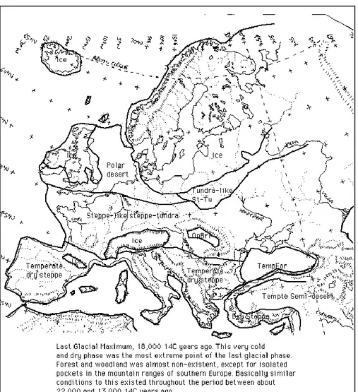
In Europe, the last glacial maximum (LGM), about 18,000 years ago, led to the
formation of a huge glacier that covered Britain and northern Europe and an icecap on top
of the highest mountain ranges such as the Pyrenees, the Alps and the Caucasus (Frenzel,
1973; Nilsson, 1983). At the edge of the glaciers was the tundra, which covering Europe
(Adams and Faure, 1997; Tzedakis et al., 2002) (Fig. 1).
The glaciations caused great changes in the distribution of species, with alternating
periods of expansion and contraction. The advance of glaciers and of permafrost led to the
loss of different habitats, with the consequent extinction of local populations and/or their confinement in areas called “glacial refuges”.
These represent areas where the temperate fauna and flora founded conditions
(habitats) suitable for their survival during adverse climate periods.
During the interglacial periods, i.e. after the Holocene climatic warming,
11 1998), and rapidly colonizing repeatedly distant areas (Hewitt, 2000) This is especially true
for taxa today having both northern and southern distributions and that have thus benefited
from newly available sites to colonize (Afzal-Rafii and Dodd, 2007).
However, in northernmost regions, expansion and founder effects are expected to
undermine allelic richness and heterozygosity of colonizing populations (Petit et al.,
2003), while southern regions since free from icecap and permafrost soils, would have
permitted much more stable population dynamics for many species with resulting higher
genetic diversity (Hewitt, 1996, 2000).
The Mediterranean region, in particular, has constituted a global refuge for relict
plants where floristic exchange and active speciation were favorite and at present the Mediterranean Basin is believed one of the world’s major biodiversity hotspots.
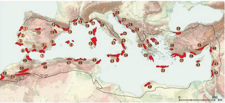
Recently, Médail and Diadema (2009) identified 10 Mediterranean regional
hotspots, representing main areas of plant biodiversity and including 52 putative refuges
(Fig. 2). About 50% of them are present in Iberian, Italian and Balkan peninsulas,
supporting the key role played during both glacial and interglacial periods by the three
major peninsulas and demonstrating as from these refuges started each colonization phase
that have marked the expansion periods in interglacial stages.
Conifers and, particularly, some species belonging to the Pinus genus, were the
most important components of the above peninsular refuges from which they plan the
12 1.4 Pinus laricio Poiret: a complex and interesting Mediterranean forest tree species
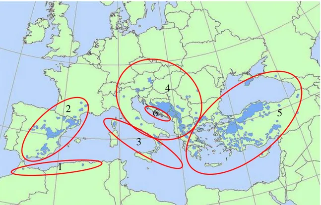
Among pine species largely present in the Mediterranean Basin, European black
pine (Pinus nigra Arnold), belonging to the Pinaceae family, is considered a relict species
pioneer that has differentiated itself in a very large and fragmented distribution area,
extending from Asia Minor in the east through the Balkans to western habitats on the
Iberian Peninsula and in North-Western Africa (Gaussen et al., 1993; Vidakovic, 1991).
Indeed, the variability in morphological, physiological and ecological traits of
Pinus nigra have led to consider this species as a complex of six allopatric subspecies: Pinus nigra ssp. nigra, ssp. dalmatica, ssp. pallasiana, ssp. mauritanica, ssp. salzmannii and ssp. laricio Poiret (Bogunić et al., 2011; Quézel and Médail, 2003) (Fig. 3).
The first black-pine-type fossils date to the Miocene, about 20 million years ago.
The ice cycles that shaped the Quaternary period in Europe are believed to have been
responsible for the currently very discontinuous range of this species. However, studies
using morphological and genetic markers have confirmed the common phylogenetic origin
of all black pines.
However, Pinus laricio Poiret is treated as the most divergent subspecies of Pinus
nigra and, some scientists, according to fossil records (Studt, 1926; Stojanoff and
Stefanoff, 1929), morphological (Gaussen et al., 1993), chemotaxonomical-anatomical
(Fineschi, 1984) and karyological (Cesca and Peruzzi, 2002) studies, regard laricio pine as a taxonomically independent species.
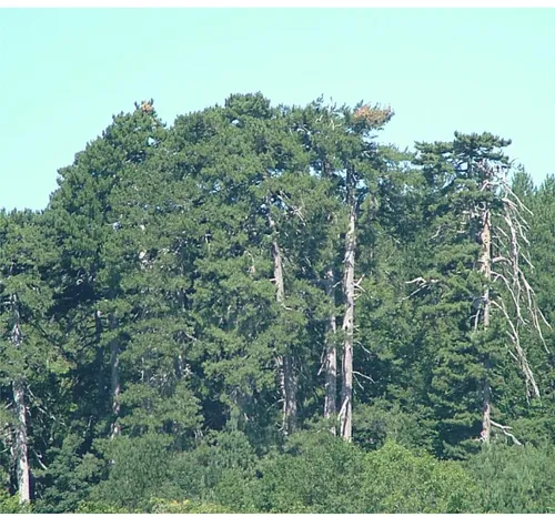
The species grows up to 50 m tall, with a trunk that is usually straight and gradually
13
up to 180 cm, in oldest plants. It has very high longevity mainly compared with Pinus
nigra: 4-5 centuries in isolated plants (Fig. 4).
Pinus laricio is a monoecious wind-pollinated species, and its seeds are wind
dispersed. The megasporangiate strobili occur predominantly high in the crown and near the ends of branches in the mid- or lower crown, and the microsporangiate strobili are borne predominantly on the interior and lower portions of the crown.
The microsporangiate strobili contains pollen grains while the macrosporangiate strobili contains ovules. Each ovule has multiple archegonia and may be pollinated by a different number of pollen grains. Multiple archegonia and multiple pollination events also provide an opportunity for competition and selection among embryos within the ovule, since only one usually survives to germinate.
Nevertheless, in Pinus laricio, such as in other Pinus species, the lack of self-incompatibility mechanisms provides a major flexibility in mating system that could be affected by elevate levels of inbreeding than outcrossing and events of self-sterility (Richardson, 2000).
Pinus laricio trees reach sexual maturity at 20 - 30 years in woods while at 15 - 18
years in marginal or isolated plants (Avolio, 2003).
In addition, it is a termo-xerophile species, though needs of bioclimatic conditions of humid (800-1,500 annual rainfall) to counter the summer aridity. The values of the mean annual temperature range from -2°C to 25°C, registered in January and August, respectively. Moreover, it is clearly a heliophile and pioneer species able to colonize open
ground (Quézel and Médail, 2003). For reproduction it needs a high degree of lighting and
the presence of poorly differentiated soil, not too rich in humus; when Pinus laricio finds these conditions form pure and unpeers woods.
14 Pinus laricio naturally occurs in restricted and discontinued areas in Calabria, Sicily and Corsica. In Calabria it grows on the Aspromonte mountain and mainly on the
Sila plateau where laricio pine forests cover 4,000 ha and 40,000 ha, respectively,
characterizing the landscape from 900 m up to 1,700 m above sea level, but with an
environmental optimum in lower mountain plan, slopes hot, arid and siliceous soils by
granitic origin.
The current distribution of populations configure how much of them remains of the
largest coating forest of southern Italy, the so-called "Silva brutia" of the Romans (Avolio
and Ciancio, 1985). The remnants forest of Pinus laricio in Sicily and Corsica cover 4,000
ha and 21,000 ha, respectively.
In Sicily, the tree forest of Pinus laricio grows on lower differentiated soil of
volcanic origin while in Corsica almost exclusively on granitic acid soils or sandy soils.
In addition, in Sicily, on the eastern slopes of Etna, pure populations of the Pinus
laricio are located between 1,200 m to 2,000 m above the sea level while in Corsica the of altitude levels ranged from 1,000 m up to 1,800 m above sea level.
Pinus laricio in Calabria is slightly more tolerant to limestone soils compared to those present in Corsica. Moreover, Pinus laricio in Corsica avoids the dry soils, those are
too acids and with high humidity, but it can grow on clay soils. The Corsican pine trees
also have a certain resistance to the action of the sea winds.
Finally, laricio pine is widely used in commercial production of hybrids in forest
regeneration due to its high survival rate. Wood is durable and rich in resin, easy to
process, and is appreciated for building and roofing because of its straightness and thin branches. If properly thinned, its low amount of duramen makes it a fine carpentry and
15 government and private sector are focusing on the use of Pinus laricio as a source of
16 In-depth genetic studies about the Pinus laricio Poiret natural populations present in Calabria, Sicily and Corsica were never carried out, though the high forestry,
phytogeographical, landscape and environmental interest on this species.
The key objective of this study is to estimate genetic polymorphism level and
distribution, and characterize population structure of Pinus laricio Poiret, using
microsatellite loci, and relate the detected patterns to available information about the life
history of the species and landscape characteristics.
The accurate characterization of the Pinus laricio population structure within its native
range is further needed to develop appropriate management or silvicultural strategies and,
17 3.1 Study site and plant sampling
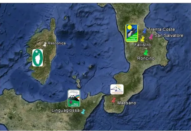
Green tissues (needles) used in this study were collected from seven uneven-aged
populations of Pinus laricio, four of them were from the Sila’s National Park, namely
Fallistro (FAL), Roncino (RON), San Salvatore (SAN) and Trenta Coste (TRE); one from
the Maesano area (ASP), within the Aspromonte’s National Park and one from the
Linguaglossa territory (ETN), within the Etna’s Regional Park. Finally, Corsican pine
individuals (COR) were collected from Restonica Valley in the vicinity of Corte's city,
within Regional Natural Park of Corsica (Fig. 5, Tab. 2).
A total number of 459 individuals were sampled for all populations, following a “random and non-contiguous” method for each plant.
Based on dendrometric information, obtained by operators of CRA-SAM
(Consiglio per la Ricerca e la Sperimentazione in Agricoltura - Unità di ricerca per la
Selvicoltura in Ambiente Mediterraneo), sampled individuals from Sila, Sicily and
Aspromonte were subdivided into four age classes, considering the tree-trunk diameter at
breast height (DBH): 1) Fustaia Stramatura (FS), including trees with diameter > 300 cm
and more than 200 years old; 2) Fustaia Matura (FM), comprising individuals 120 years
old with a circumference range of 180-300 cm, 3) Fustaia Adulta (FA), with trees 80 years
old and 90-150 cm of circumference range and 4) Novelleto (NV), with juvenile
18 An additional age class, Fustaia Giovane (FG), including trees with diameter 60-80
cm and a mean age of 40 years, was sampled only for FAL population. All the 11 Corsican
samples came from NV individuals.
Furthermore, geographic coordinates were obtained for each sampled individual
with a GPS (Global Positioning System) receiver (Leica-Magellan); flat coordinates were
recorded in Gauss–Boaga coordinate system and transformed into UTM geographic
coordinate system.
Individually sampled needles were conserved at -80°C until processing.
3.2 DNA extraction and microsatellite analysis
Total genomic DNA was isolated from needles of individual trees using the
DNeasy Plant Mini Kit (Qiagen). Screening for polymorphism was conducted with 5
chloroplast (cp) (Pt30204, Pt36480, Pt45002, Pt71936 and Pt87268), 1 mitochondrial (mt)
(Nad3-1) and 3 nuclear (nu) (PtTX4001, PtTX3107 and SPAG7.14) microsatellite primer
pairs (Tab. 3), originally designed for Pinus taeda and Pinus sylvestrispopulation genetic
studies (Vendramin et al., 1996; Soranzo et al., 1998; Soranzo et al., 1999; Auckland et al.,
2002).
PCR was performed using both a Perkin Elmer GeneAmp PCR System 9600
thermal cycler and an Eppendorf Mastercycler Pro with conditions varied for different
primers and forthe presence of the forward onesVIC, 6-FAM, NED and PET labeled.
Each amplification reaction contained approximately 10 ng genomic DNA, 1X
19 mM MgCl2, 0.2 mM dNTP mix, 1 pmol/µL of each primer, 1 U Red Taq DNA polymerase
(Euroclone) and deionised water to a total reaction volume of 20 µL.
PCR conditions using mt- or cpSSR primers were as follows:
Initial denaturing step of 3 minutes at 94°C 30 cycles of:
o 94°C (30 seconds) denaturation
o 55°C (30 seconds) annealing
o 72°C (30 seconds) extension
Final extension period of 5 minutes at 72°C.
The touchdown PCR conditions with nuSSR primers were set as follows:
Initial denaturing period of 3 minutes at 94°C 10 touchdown cycles:
o 94°C (30 seconds) denaturation
o 60°C (30 seconds) annealing, declining 1°C every cycle until
50°C o 72°C (30 seconds) extension 30 cycles o 94°C (30 seconds) denaturation. o 50°C (30 seconds) annealing o 72°C (30 seconds) extension Final extension step of 5 minutes at 72°C
20 Particularly, for SPAG 7.14 primer pair, the touchdown cycles were 5 and
annealing temperature started with 55°C instead of 60°C.
Amplicons were visualized through 3% agarose gel electrophoresis in order to
determine presence or absence of specific products and, then, purified with QUIAquick
PCR Purification Kit (Qiagen).
Next sequencing analysis on an ABI Prism 310 Sequencer (Applied Biosystems)
was carried out to confirm both the presence of the microsatellites in the amplified
fragments and the fact that variation in length was due to different numbers of repeats
within the microsatellite regions.
3.3 Microsatellite genotyping
Aliquots of each fluorescent dye labeled PCR product (0,5 µL) were additioned at
Formamide (11,5 µL) and internal size standard LIZ 500 (0,5 µL) (Applied Biosystems).
After denaturation for 5 min at 95°C, labeled amplicons were separated by capillary
electrophoresis on an Applied Biosystems Prism 3730XL Genetic Analyser using filter set
G5.
The data were analyzed using Peak Scanner v. 1.0 software (Applied Biosystem).
Each resulting peak was considered as an allele at a codominant locus and the genotype of
21 3.4 Data analyses: within and among population diversity and genetic structure of populations
Main values of chloroplast and nuclear genetic diversity [allelic frequencies,
number of alleles (Na), number of effective alleles (Ne), haplotype diversity (H), observed
heterozygosity (Ho), expected heterozygosity (He), fixation index (F) and inbreeding
coefficient (FIS)] were computed with GenALEx version 6.4 software (Peakall and
Smouse, 2006).
Allelic richness was calculated with the FSTAT version 2.9.3.2 program (Goudet,
2001), using the rarefaction approach proposed by El Mousadik and Petit (1996) to correct
for differences in sample size. Standard sample size consisted of 11 individuals, which
corresponded to the smallest Pinus laricio population sampled (COR) (Tab. 2).
A test for Hardy-Weinberg (H-W) Equilibrium was performed using the program
GENEPOP version 4.1 (Rousset, 2008) and according to Fisher (1935), to determine
whether the observed genotypes are consistent with the expectations under random mating.
When significant deficiencies of heterozygotes from H-W expectations were found,
the presence of a relatively high frequency of null alleles was suspected.
Therefore, loci with high frequencies of null alleles were identified by estimating
null allele frequencies for each locus and each population, using the software FREENA
(Chapuis and Estoup, 2007).
Values > 0.19 of null allele frequency have been considered as a threshold over
which significant underestimate of He due to null alleles can be found (Chapuis and
Estoup, 2007).
An Analysis of Molecular Variance (AMOVA) (Excoffier et al., 1992; Michalakis
22 by computing ΦPT and FST estimators, assuming the infinite allele model (IAM), and the RST estimator, assuming the stepwise-mutation model (SMM) (Slatkin, 1995). Statistical significance of all the ΦPT, FST and RST estimators were tested using 10,000 permutations.
GENETIX version 4.04 software ( Belkhir et al., 2001), also, was used to estimate
Gst value.
In addition, a Principal Coordinate Analysis (PCA), also available in GenALEx
version 6.4 program, was conducted using Nei’s unbiased genetic distance pairwise
population matrix to determine whether observed patterns in the molecular data support the
partitioning of the Pinus laricio samples into specific groupings.
The degree of isolation-by-distance was assessed by testing the association between
geographic distances (log-transformed) and genetic distances (expressed as linearized ΦPT
and FST/1-FST for cpSSR and nuSSR, respectively) for all pairs of populations. The
statistical significance of the associations was tested based on a Mantel test (Mantel, 1967).
Spatial Autocorrelation Analysis was conducted for each Pinus laricio population
and for both cpSSR and nuSSR to test the existence (H1) or not (H0) of a non-random
distribution of genotypes in space. The analysis, performed comparing genetic distance and
geographic genetic distance matrices, was based on the parameter of spatial autocorrelation
(r), that should be > or < than 0, estimated with random permutations and bootstraps, selecting two different options of “Even Distance Classes” and “Even Sample Sizes”.
Finally, Bayesian clustering methods were applied to infer the number of genetic
units and their spatial delimitation.
Bayesian clustering methods use genetic information to ascertain population
membership of individuals without assuming predefined populations. They can assign
23 multilocus genotypes. The methods operate by minimizing H-W and linkage disequilibria,
and the assignment of each individual genotype to its population of origin is carried out
probabilistically (Chen et al., 2007).
Among Bayesian methods, STRUCTURE 2.3.3 program (Pritchard et al., 2000;
Pritchard et al., 2010) was used to identify clusters (K) of genetically similar individuals.
The analysis was conducted under the admixture model and the option of correlated allele
frequencies between populations.
Five independent runs (iterations) were performed for each K, that varied from K =
1 to 10. The maximum number of clusters used was greater than the number of
populations, for detection of potential substructuring within samples. All runs were
performed with burn-in length of 10,000 and repetition number of 100,000 iterations.
The number of clusters was determined using the ad-hoc statistic ΔK according
with Evanno et al. (2005) and based on the rate of change of log likelihood of data [L(K)]
between consecutive K values used to select the optimal K.
TESS software (Durand et al., 2009) uses a Hidden Markov Random Field model
that assumes that the log-probability that an individual belongs to a particular cluster given
the cluster membership of its closest neighbors is equal to the number of neighbors
belonging to this cluster.
The probability that two neighboring individuals belong to the same spatial cluster
is controlled by a parameter known as the “interaction parameter” (Ψ). Any non-zero value
introduces spatial dependence, with default value set to 0.6.
Three quantities, that is, a graph specifying the set of neighbors of each individual,
the interaction parameter and the maximum number of clusters (K), were involved in the
24 number of clusters that best fit the data is, thus, chosen by the user from the statistical
Deviance Information Criterion (DIC).
In our TESS analysis using both cpSSr and nuSSR data set, a Ψ value = 0.6,
without admixture and with admixture, was tested. In addition, 9 runs were performed for a
total number of sweeps of 50,000, a burn-in number of sweeps equal to 10,000, with the
number of clusters K from 2 to 10, and 3 repetitions (for each data set) for a total of 27
runs. Then, the DIC values of the 27 runs were averaged.
GENELAND program implements a method developed by Guillot et al. (2005) that
quantifies the amount of spatial dependence in a data set, estimates the number of
populations, assigns individuals to their population of origin, and detects individual
migrants between populations, while taking into account uncertainty on the location of
sampled individuals.
The spatial domain of the sample is partitioned into a union of a random number of
polygons by Voronoi tessellation that is randomly assigned to one of potential K spatial
clusters. K is considered unknown, with maximal value (Kmax) input by users, and estimated
by the algorithm. When polygons are assigned to different spatial clusters, the joint
probability that any two polygons belong to the same spatial cluster decreases with
geographical distance between them.
Estimates of K (the number of spatial clusters) and individual assignment
probabilities are obtained using a Markov Chain Monte Carlo (MCMC) algorithm, an
iterative procedure which starts from arbitrary values for all unknown parameters and
25 In our analysis, 10 indipendent runs were performed for K from 1 to 50. Each run
consisted of 105 MCMC iterations with a thinning interval of 100, using correlated allele frequencies and spatial information.
In order to obtain the posterior probabilities of population membership of each
individual and each spatial area, 10 runs were then post processed with a burn-in of 104 MCMC and 100 pixels along the X-axis and 200 pixels along the Y-axis. Then, the
consistency of the results was visually checked by comparing the outputs across the 10
runs.
BARRIER program (Manni et al., 2004) was used to verify the presence of genetic barriers among populations. This software implements the Monmonier’s algorithm based
on a neighbor graph (such as a Delaunay triangulation) between sampled populations or
individuals, and calculates the genetic distances associated with each edge of the graph.
The algorithm builds growing barriers from the edge with the largest genetic distance, and
extends it to the adjacent edges associated with the next largest genetic distance.
DIYABC (Cornuet et al., 2010) is a inference program based on Approximate
Bayesian Computation (ABC), in which scenarios can be customized by the user to fit
many complex situations involving any number of populations and samples.
Such scenarios involve any combination of historical population events
(divergences, admixtures, population size fluctuations). DIYABC can be used to compare
competing scenarios, estimate parameters for one or more scenarios and compute bias and
26
4. Results
4.1 Chloroplast microsatellites analysis
4.1.1. Genetic diversity estimates
Three out the five used cp markers (Pt30204, Pt71936 and Pt87268) (Tab. 3) were
found polymorphic in all populations studied, although the degree of variability was
different at each locus. Indeed, the number of amplified size variants (or alleles) for each
polymorphic site ranged from 6 to 11, the maximum of which was showed by the locus
Pt30204 with 11 size variants followed by Pt87268 and Pt71936 (Tab. 4).
On a population/ per locus basis the mean number of alleles (Na) was 5.91, a higher
value compared with that previously reported for Pinus nigra Arnold (Naydenov et al.,
2006).
The size of all the detected alleles ranged from 138 to 173 bp, reflecting a large
difference in the number of repeats between the different alleles (Tabs. 3, 4).
4 out of 27 size variants identified at the 3 loci occurred at low frequencies (<1%) and, thus, represent a group of “rare size variants” (Tab. 4).
Two of this rare alleles (alleles 138 at locus Pt30204 and allele 145 bp at locus
Pt71936) (Tab. 4), are also “private”, that is, exclusively present in individuals of TRE and
ASP populations, respectively.
Instead, the other rare size variants such as alleles 167 bp and 173 bp at locus
27 The most common size variants were fragments 143 bp at locus Pt30204 with a
frequency of 31.3%, 147 bp at locus Pt71936 with a frequency of 57.5% and 170 bp at
locus Pt87268 with a frequency of 51.9% (Tab. 4).
The mean number per locus and populations of effective alleles (Ne) was 3.05, a
genetic variability value comparable with the allelic richness parameter (Ar = 4.52) (Tab.
5), calculated on minimum sample size of 11 aploid individuals.
Haploid diversity (h) was on average 0.65 with the largest value observed in the
Maesano population (ASP = 0.74), while Fallistro stand showed the lowest variability
(FAL = 0.60) (Tab. 5).
The 27 size variants were combined in 84 different haplotypes, 25 of these were
found in the FAL population versus 34 present in the ETN stand. Only 8 haplotypes was
detected in the Restonica population (COR), very likely due to small size sampling (Tab.
5).
39 out of 84 haplotypes were unique or private (frequency <1%) and are due to the
presence of rare size fragments and/or rare combinations of size fragments. These unique
haplotypes were found in all areas of the Pinus laricio natural distribution, with exception
for the population located in the Corsican territory. In particular, three and eight unique
haplotypes occurred in the SAL and ASP/ETN stands, respectively (Tab. 5).
The effective number of haplotypes in each stand ranged from 6.37 in Corsica to
20.5 in Sicily (Tab. 5). Furthermore, within the Calabrian area, Maesano (ASP) exhibits
the largest percentage of individuals with private haplotypes (21%) versus only the 10%
detected in the FAL stand (Tab. 5).
Three haplotypes (h-18, h-62 and h-68 in Table 6) are common to all Pinus laricio
28 haplotype h-41 (11.6%) was found in the Sila, Etna and Corsica stands but not in the
Maesano (ASP) population; conversely, the haplotype h-72 (frequency 3.5%) was detected
in the populations from Sila, Aspromonte and Etna but it was absent in the Corsica stand
(Tab. 6).
Overall, the predominant haplotypes which occur in at least ½ of the analyzed
populations correspond to 45.3% of the laricio pine genetic structure.
Intra-population gene diversity values (He) based on haplotype frequency varied
from 0.917 in FAL to 0.966 in ETN (Tab. 5) while the total haplotype diversity calculated
across all populations was 0.942 on average.
4.1.2. Genetic variability among populations
Considering the data generated with 3 cpSSRs, in the above cited laricio pine
stands, an analysis of molecular variance (AMOVA) was conducted to partition the cpSSR
variance into within- and among populations (Tab.7). The above analysis revealed that
3.4% of the variation was found among populations with 96.6% of the diversity being
expressed within populations.
The PT value is slightly lower compared with that previously reported for Pinus
nigra Arn. and other Pinus species (Naydenov et al., 2006; Bucci et al., 2007; Dzialuk et al., 2009). Indeed, the calculated FST and GST that estimate the degree of population
differentiation were 3.4 and 4.1%, respectively, confirming the AMOVA results. The slight
discrepancy is probably due to the different principles of G-statistics and
29 The AMOVA analysis was also performed using pairwise comparison of
populations between two (or more) different areas, revealing an higher molecular variance
value (5.3%) between Sila and Aspromonte populations followed by lower differentiation
values for Sila-Etna (2.7%) and Aspromonte-Etna (1.9%) comparisons (Tab. 7).
Genetic distance between populations, calculated according Nei (1978), varied
from 0.023 between SAL and TRE to 0.227 between SAL and ASP (Tab. 8). Particularly,
the smallest values, ranging from 0.023 (TRE-SAL) to 0.064 (RON-TRE), were observed
within Pinus laricio stands located in the Sila National Park (Tab. 8).
According to AMOVA analysis, the highest dissimilarity values were, thus, found
between Sila and Aspromonte populations (Tab. 8), while the Calabrian populations
displayed high genetic similarity with those of the Linguaglossa (ETN) and Restonica
(COR).
The average gene flow (Nm) is estimated to be equal to 14.21 migrants per
generation.
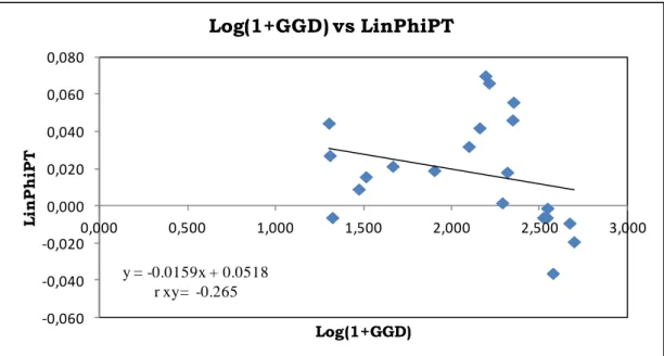
A Mantel (1967) test was performed to verify the hypothesis about the spatial
pattern in the distribution of chloroplast gene diversity at the stand level. To this end, the
log matrix of geographic genetic distance (x data) and the linearized ΦPT matrix (y data)
were associated. A negative and not significant relationship (rxy = -0.265, P < 0.05) was
found (Fig. 6), indicating the absence of a pattern of isolation by distance among Pinus
laricio populations within their natural area of distribution.
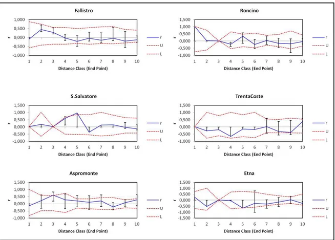
In addition, to verify the hypothesis of the presence (H1) of a non-random
distribution of genotypes in space, an analysis of spatial autocorrelation was carried out for
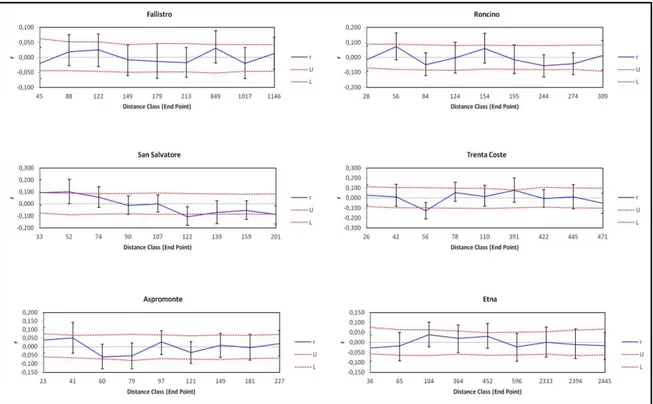
30 The results of this analysis showed, in each population and for both the “Even
Distance Classes” (Fig. 7) and “Even Sample Sizes” (Fig. 8) options used, a value of the
parameter of spatial autocorrelation included between Upper (U) and Lower (L)
confidence limits bound the 95% confidence interval about the null hypothesis (H0) (r =
0). Thus the non-random distribution of genotypes was discarded.
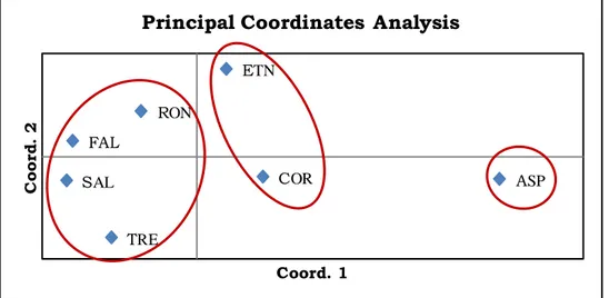
Next, for better interpretation of the genetic distances found among laricio pine
natural populations, the Principal Coordinates Analysis (PCA) was conducted. This analysis, performed on Nei’s unbiased genetic distance matrix and based on 27 different
size variants, clearly distinguished the seven laricio pine stands into three main groups, one
including the FAL, TRE, SAL and RON populations, the second group comprising the
Linguaglossa (ETN) and Restonica (COR) populations and the third cluster including the
Maesano (ASP) stand alone (Fig. 9).
In the PCA analysis, the first coordinate explains 73.24% of unbiased genetic
distance while the second coordinate explains 13.82%, with a total value on the two main
coordinate equal 87.06% of the same parameter.
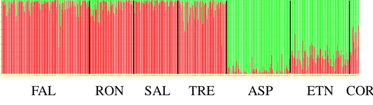
Also, the population structure analysis of natural populations of Pinus laricio was
carried out using a Bayesian clustering algorithm, implemented in the TESS software
(Durand et al., 2009), that incorporates spatial information when identifying clusters of
individuals.
The TESS software allows the testing of different values of the spatial dependent
parameter Ψ that weights the relative importance given to spatial connectivities. A value of Ψ = 0.6 was tested in this analysis.
31 For Ψ value considered in this analysis, 9 runs for K from 2 to 10 were performed,
with a total number of sweeps of 50,000, a burn-in number of sweeps equal to 10,000 and
3 repetitions for a total of 27 runs.
Then, the DIC values of the 27 runs with the smallest DIC were averaged. In
plotting the average DIC values versus K (from 2 to 10) an inflection point at K = 5 was
obtained. Sometimes the effective number of clusters in the data may be a smaller value of
K and, in this case, the best K seems to be 2 because for this value, in the model without
admixture, was observed the best barplot stabilizes, thus indicating the presence of a
moderate spatial correlation between individuals (Fig. 10).
Therefore, the seven natural populations of Pinus laricio are grouped into two main
clusters: the first cluster contained all the four Sila populations of laricio pine while the
second cluster included the remaining stands of Maesano, Linguaglossa and Restonica.
4.1.3. Evolutionary inferences of Pinus laricio populations based on cpSSRs.
A DIYABC analysis, a variant of ABC analysis (EXcoffier et al., 2005), was
performed considering two main populations of Pinus laricio: the first including all the
Sila National Park populations (Pop 1 in Fig. 11) while the second comprises the
populations of Restonica, Linguaglossa and Maesano (Pop 2 in Fig. 11). In the DIYABC
analysis were tested three possible scenarios to describe the demographic evolution of
natural populations of Pinus laricio through time.
In the first scenario, it was assumed that Pop 2 was separated from Pop 1 at time
32 population at time T3; at time T2 this population was subject to bottleneck that originated
the Pop 1 at time T1. Finally, in the third scenario, it was assumed that Pop 2 was
separated from an ancestral population at time T2 and at time T1 Pop 1 was separated from
Pop 2 (Fig. 11a).
These scenarios were tested on 3,000,000 simulations, computing the main
parameters as PCA (Principal Component Analysis), logistic regression, the values of FST,
mean genic diversity and the posterior distribution of parameters. The results of this
analysis, and for each parameter analyzed, showed that the third scenario was better
supported than the other two scenarios because the most observed summary statistics are
well in the range of those simulated (Fig. 10 and data not shown).
Moreover, it was possible to plot the values of T1 and T2 on the time scale not in
generations but in number of mutational events, based on the posterior distributions, with
ABC analysis. So, for the third scenario the values of T1 and T2 was respectively
2.40E+002 and 5.47E+003 (data not shown).
Knowing the estimated time values of mutational events and the years for a
reproductive generation in Pinus laricio (20 years), the time T2 of separation of Pop 2
from ancestral population (109,000 years ago) and the time T1 of separation of Pop 1 from
33 4.2 Nuclear microsatellites analysis
4.2.1 Allelic diversity of microsatellite loci and genetic variation within populations
Three published primer pairs (Auckland et al., 2002; Soranzo et al., 1998) flanking
nuclear microsatellites were employed to investigate the level of genetic variation among
the 7 Pinus laricio populations sampled in this study.
The three markers (SPAG7.14, PtTX4001 and PtTX3107) were found to be
polymorphic in all analyzed populations, producing a variable number of alleles per locus
(Tab. 9).
Indeed, between 6 (at locus PtTX3107) and 38 (at locus SPAG7.14) size variants
were identified with an average (Na) for all loci and populations of 11.48 (Tab. 10). The
effective number of allele (Ar = allelic richness), calculated on minimum sample size of 11
diploid individuals, ranged from 5.33 in the Restonica population (COR) to 7.05 in the
RON stand with an average of 6.56 (Table 10).
A total of 52 size variants at the 3 loci were identified, of which 15 with frequencies <1% and, thus, considered as “rare” alleles. Four of them are also “private”
since they are present in ETN (alleles 222 and 244 bp at locus SPAG7.14), RON (allele
213 bp at locus PtTX4001) and SAL (allele 232 bp at locus SPAG7.14) trees (Tab. 9). The remaining “rare” alleles (8, 2 and 1 alleles at the SPAG7.14, PtTX4001 and
PtTX3107 loci, respectively) were found common to two or more Pinus laricio
34 The most common size variants, namely the 202 bp (at locus SPAG7.14), 211 bp
(at locus PtTX4001) and 160 bp (at locus PtTX3107) alleles, were found with a frequency
of 17.9%, 50% and 71.6%, respectively (Tab. 9).
Examination of intra-population genetic diversity revealed the lowest value of Nei’s
unbiased genetic diversity (He = 0.628) among individuals from FAL population while
samples from ASP stand showed a highest variability (He = 0.701) (Tab. 10).
In all sampled populations, the observed heterozigosity (mean Ho = 0.528) was
lower than expected (mean He =0.674). The difference determines a significant positive
value for mean Fixation Index (F = 0.204) (Table 10) and inbreeding coefficient (FIS =
0.197) (Table 11), that could very well be attributed tonon-random mating and null alleles.
Therefore, FREENA software (Chapuis and Estoup, 2007) was used to recompute
the null allele frequencies and, thus, adjust F estimates.Frequencies lower than 0.19 were
obtained for all loci for each sampled population, except for COR stand, where null allele
frequencies higher than 0.2 were only found at the loci SPAG7.14 and PtTX4001 (Tab.
12).
A recalculation of all the F-statistics were also made and no significant differences
were observed. For example, the global FST (Weir, 1996) is generally calculated in order to
estimate the proportion of the total genetic variation due to the differentiation among
populations. Taking or not into account the null allele frequencies, the global FST values
were 0.018 and 0.019, respectively (Tab. 11). Moreover, a χ2
test using Fisher’s method as implemented in GENEPOP 4.1
software (Rousset, 2008) was performed to evaluate if deviations from the H-W
equilibrium were probabilistically significant or no. We found very highly significant tests
35 observed in all the Pinus laricio populations is due to inbreeding between closely related
individuals.
Furthermore, to investigate the potential effects of inbreeding over long periods of
time, individuals from each Pinus laricio populations were partitioned in diameter or age
classes, and F values computed and compared (Tab. 13). A considerable excess of
heterozygotes was only found for trees 10-15 years olds (NV in Tab. 13) belonging to the
FAL and ETN stands, as indicated by the negative Fixation Index obtained (0.024 and
-0.104, respectively).
Instead, from 80 years old individuals (FA) to those 120 years olds (FM), the
heterozygosity levels (radically) declined and an excess of homozygous is recorded (Tab.
13).
4.2.2. Genetic diversity among populations
Global and hierarchical population genetic structure were evaluated by analysis of
molecular variance (AMOVA) (Excoffier et al.,1992) under (IAM) and (SMM) models
(Tab. 14).
The AMOVA-IAM model analysis revealed that 2,1% of the variation was found
among populations with 97,9% of the diversity being expressed within populations. The
FST value was comparable to the Nei’s coefficient GST (3.1%) but lowest than RST value
(9.2%) obtained when the genetic differentiation among the seven laricio pine populations
36 The average gene flow (Nm), based on the FST value via AMOVA, was equivalent
to 11.65 migrants per generation, with RON stand showing the greatest value (data not
shown).
AMOVA analysis was also performed on pairwise populations, evaluating the
differences in the FST parameter. The comparison between ETN, ASP and Sila populations
and the COR stand showed values of molecular variance among populations ranging from
1.9% to 3.3% while no genetic difference seems to emerge between ASP-ETN populations
(Tab. 14).
The greatest values of genetic distance, estimated according to Nei (1978), were
observed between COR and each other laricio pine stand, sampled in this study (Tab. 15).
Particularly, the topmost dissimilarity was found with FAL (0.246), the latter also
genetically different with respect to ASP stand (0.097). Moderately high distance values
were recorded among the four populations within Sila National Park while ASP and ETN
populations were found closely related genetically (0.021) (Tab. 15).
To ascertain whether there is a statistically significant relationship between genetic
and geographic distance, a Mantel (1967) test was performed. By plotting the genetic
distance among population pairs as a function of the geographic distance between those pairs, no significant correlation was found (rxy = 0.266, P < 0.05) (Fig. 12), thus, rejecting
the assumption of an isolation by distance among Pinus laricio natural populations here
sampled.
Each single population of Pinus laricio was further tested by a spatial
autocorrelation analysis to verify the hypothesis (H1) of a non-random distribution of
genotypes in the space. The estimated parameter of spatial autocorrelation (r), if in
37 Values of r = 0 (P < 0.05) were obtained for each laricio pine population, thus,
indicating that the individual genotypes in space are randomly distributed in space (Figs.
13, 14).
Stand genetic structure was tested using three different approaches. First, the Principal Coordinate Analysis (PCA), performed on Nei’s unbiased genetic distance matrix
and based on 52 different size variants, showed that the 7 sampled populations of Pinus
laricio were separated in three main groups (Fig. 15).
Group I contains three out the four populations from the Sila National Park (RON,
SAL, TRE) as well Maesano (ASP) and Linguaglossa (ETN) stands. Group II and III
include FAL and COR populations, respectively. In the PCA analysis the first two
principal axes explain in total 86.41% of unbiased genetic distance (Fig. 14).
Next, Bayesian clustering algorithms such those implemented in TESS 2.3 and
GENELAND programs were used for inferring laricio pine population structure (Durand et
al., 2009; Guillot et al., 2005). Both programs include spatial coordinates into classical
analyses based on multilocus genotypes.
In TESS analysis, a Ψ value of 0.6, without admixture and with admixture, was
tested. For the above Ψ value, number of runs and clusters were performed as reported in
Methods.
Graphical outputs by plotting the average DIC values versus K (from 2 to 10)
showed an inflection point at K = 5, without admixture model, and an inflection point at K
= 6 with admixture model.
However, when the assignment probabilities of individuals to different clusters
were displayed in a bar chart, the barplot stabilizes at K = 2 for both models, thus, showing
38 Therefore, the natural populations of Pinus laricio were assigned to 2 main clusters:
cluster 1 includes all Sila populations while cluster 2 contains the remaining stands of
Maesano (ASP), Linguaglossa (ETN) and Restonica (COR) (Fig. 16).
The ability of the GENELAND program (Guillot et al., 2005) to infer population
structure is well recognized compared to other spatially implicit clustering methods,
particularly, when genetic differentiation is weak, a typical situation for trees collected
over a large geographic area.
As result of my GENELAND analysis, the best number of clusters along the chain
(after burn-in) for the seven populations of Pinus laricio analyzed in this study was K = 2
(Fig. 17a), such as TESS outputs. Two main clusters were evident, the first including the
four populations of Sila plateau, the second one ASP, ETN and COR stands (Fig. 17b).
Furthermore, to test the effect of the landscape characteristics on the genetic
structure of Pinus laricio populations, an additional method implemented in BARRIER software, based on the Monmonier’s maximum difference algorithm, was used (Manni et
al., 2004).
Nei’s genetic distances were used to generate 10 bootstrapped matrices allowing to
identify one most supported genetic barrier (Fig. 18) that separates the FAL population
from the other Pinus laricio populations located in the Sila National Park.
A further Bayesian clustering approach, implemented in STRUCTURE software
(Pritchard et al., 2000; Pritchard et al., 2010), was used as final approach for population
structure analysis.
This program performs a multilocus analysis on the genotypes of individuals
sampled in different geographical areas, but it does not require geographic information.