Lying for the Greater Good: Bounded Rationality in a Team

LYING FOR THE GREATER GOOD:

BOUNDED RATIONALITY IN A TEAM

OKTAY SÜRÜCÜ

Received: June 19, 2014 Accepted: July 21, 2014 Online Published: September 18, 2014

Abstract

This paper is concerned with the interaction between fully and boundedly rational agents in situations where their interests are perfectly aligned. The cognitive limitations of the boundedly rational agent do not allow him to fully understand the market conditions and lead him to take non-optimal decisions in some situations. Using categorization to model bounded rationality, we show that the fully rational agent can nudge, i.e., he can manipulate the information he sends and decrease the expected loss caused by the boundedly rational agent. Assuming different types for the boundedly rational agent, who differ only in the categories used, we show that the fully rational agent may learn the type of the boundedly rational agent along their interaction. Using this additional information, the outcome can be improved and the amount of manipulated information can be decreased. Furthermore, as the length of the interaction increases the probability that the fully rational agent learns the type of the boundedly rational agent grows.

Keywords: bounded rationality; categorization; nudging; learning.

1. Introduction

In economic literature, one of the most commonly used assumptions about decision makers is the full rationality. When faced with an economic decision problem, a fully rational decision maker has the ability to see and understand what is feasible and what is preferable. Furthermore, he is also able to calculate the optimal course of action given these two constraints. This widely used assumption, which simplifies economic models, has received many criticisms for overlooking real life situations by ignoring cognitive limitations.

Wide literature initiated by Amos Tversky, Daniel Kahneman, and their collaborators provides us with experimental evidence that human beings depart systematically from full rationality due to cognitive limitations. These limitations affect their ability to recognize the available information on markets and their ability to compute. Herbert Simon, the originator of the phrase, defines bounded rationality as "rational choice that takes into account the cognitive limitations of the decision-maker-limitations of both knowledge and computational capacity" (Simon 1987).

Boundedly rational agents try to simplify and structure the economic decision process. A possible way to do this is to use categories. The usage of categories is also supported by psychological evidence that people in environments with abundance of information show the tendency to group events, objects or numbers into categories depending on their perceived similarities (Rosch and Mervis 1975). According to the social psychologist Gordon Allport "…the human mind must think with the aid of categories. We cannot possibly avoid this process. Orderly living depends upon it"(Allport 1954, pg 20). Both in economic and social psychological literature, there are many studies aiming to explain human behavior using categorization (e.g. see Macrae and Bodenhausen 2000 or Fryer and Jackson 2008).

The following example illustrates one possible way how the categorization process works. Consider a consumer who wants to buy a new television. There are an overwhelming number of available alternatives on the market. In order to make a decision, the consumer has to compare a long list of attributes among all products. These attributes include a wide variety of technical features (e.g. screen size, aspect ratio, resolution, contrast ratio, sound system, dimension, weight, etc.), price arrangements (price of the product, payment schedule, service fees), brand, warranty, product support, delivery service, etc. Unless the consumer is an expert on televisions, he may have difficulties in making decision because of this long list of items to consider for each product on the market.

What happens most of the time is that after eliminating the obviously undesirable alternatives (e.g. too expensive products), the consumer categorizes the rest of the alternatives so that in each category there are products with some similar attributes. At each step of the categorization process, the consumer chooses an attribute, attaches some criteria to it and partitions the set of products based on the criteria. Say, for example, he considers the screen size attribute and the criteria he attaches is if it is less than 45 inches or between 45 and 55 inches or larger than 55 inches. In this way, he partitions the products into three sets as "products with screen sizes less than 45 inches", "products with screen sizes between 45 and 55 inches" and "products with screen sizes higher than 55 inches". He continues the categorization process by choosing another attribute-criterion tuple, say resolution and a threshold for resolution. He further refines each set in his partition based on this new attribute-criterion tuple and obtains a new partition. In particular, he divides each of the three sets into two as high-resolution and low-resolution, and ends up with 6 sets (categories) in his new partition.1

Repeating this process for a number of steps, he ends up with a final partition of products.2 Each category in this partition consists of products having similar features. He chooses one product from each category as a representative and compares all the representatives. Then he considers only the category whose representative gives the maximum utility.

The final decision is made among the products in that category. This process may lead to a non-optimal decision since the consumer considers only a small subset of products (the category whose representative gives him the highest utility) rather than the whole set. Furthermore, another feature of categorization is that even if their preferences are perfectly aligned, the decisions made by different individuals may not be the same. This follows from the fact that the final partition for a consumer is most likely to be different than the final

1

Low small size, high small size, low medium size, high resolution-medium size, low resolution-big size and high resolution-big size.

2

The number of steps depends on the degree of the individual's bounded rationality. In the limit case (when the individual is fully rational, say, an expert on televisions), the number of steps is sufficiently large that each category contains only one product (finest partition).

partition of another consumer, since it depends on the number of steps and the criteria the individuals use.

The main purpose of this study is to analyze the interaction between fully and boundedly rational agents. More specifically, we focus on situations in which both agents work together in a team. The boundedly rational agent makes a decision after receiving a message from the fully rational agent and this decision determines the payoff of the team. We investigate if and how the fully rational agent can nudge, put differently, if he can stimulate the boundedly rational agent to avoid from non-optimal decisions. We show that he can achieve this goal by manipulating the information that he sends to the boundedly rational agent.

Furthermore, during their interaction, the fully rational agent can infer about the categories used by the boundedly rational agent; and hence, decrease the amount of manipulated information. The following setting about a fully rational boss and his boundedly rational namesake can be considered as a motivating example for our model. The boss is willing to buy arms for hunting animals. However, having a criminal record, he does not meet the conditions for registration of arms with the police forces. Therefore he asks his namesake, who does not have any records of criminal commitment, to buy a weapon for him. The namesake has also some connections in the weaponry black market. Therefore he can buy the weapon from either the legal or illegal market. At this point, it is important to note that the problem we are dealing with is not a principal-agent problem, but an instance of team theory initiated by Roy Radner. In principal-agent problems there is a conflict of interest giving rise to agency cost. In our setting, however, this is not the case since the preferences of the boss and his namesake are perfectly aligned.

Our paper takes as a departure point Dow (1991), where an economic decision problem for a boundedly rational agent visiting two stores and searching for the lowest price is modeled. The bounded rationality of the agent comes from his limitations in memory. More specifically, when the agent is in the second store, he cannot remember the exact price in the first store, but only remembers to which category it belongs. The agent makes a decision by comparing the price in the second store with the representative of the category to which the price in the first store belongs. Dow (1991) characterizes the optimal categorization. We depart from Dow's setting by introducing a fully rational agent and examining the interaction between the two agents.

Considering a similar setting, Chen, Iyer and Pazgal (2010) and Luppi (2006) examine the price competitions in the market and show that fully rational firms can take advantage of boundedly rational consumers. Chen, Iyer and Pazgal (2010) depart from Dow's setting by introducing two different types of consumers: totally uninformed consumers, who only consider buying from a specific store as long as the price is below their reservation value, and informed consumers with perfect memory, i.e., fully rational consumers. They characterize the Nash equilibrium of the game in which firms choose pricing strategies and consumers with limited memory choose their categories. It is shown that having boundedly rational agents in the market softens price competition. A similar setting is used by Luppi (2006), where there are rational firms on one side and boundedly rational consumers on the other side of the market. Consumers categorize the price space and make their decision based on their categories. It is shown that in the presence of boundedly rational consumers, two firms competing a la Bertrand depart from the standard equilibrium and make positive profits. The difference between these two papers and ours comes basically from the difference in the settings. In our case, the fully and the boundedly rational agents are working as a team and their common aim is to improve the outcome. In other words, the fully rational agent is not trying to take advantage of the boundedly rational agent like in Chen, Iyer and Pazgal (2010)

and Luppi (2006), but he is trying to decrease the expected loss caused by the boundedly rational agent.

Another literature strand to which this paper refers is the field of Information Transmission. Crawford and Sobel (1982) analyze costless strategic communication between a better-informed, fully rational sender and a fully rational receiver. The sender categorizes the support of messages and sends the category to which the realized message belongs instead of sending its real value. This situation arises because the players' preferences are not perfectly aligned. The receiver, after reading the signal, takes an action that affects both his and the sender's payoff. It is shown that as the preferences become more aligned, the number of categories the sender uses increases, i.e., the signal becomes more informative.

Although there have been many studies in economic literature on bounded rationality, studies on interaction between fully and boundedly rational agents are limited in number. To our knowledge, all these studies are concerned with how fully rational agents can take advantage of boundedly rational agents (see Rubinstein 1993, Piccione and Rubinstein 2003, Eliaz and Spiegler 2006). The main novelty of our paper lies in our team approach. Both types of agent work together to decrease the inefficiency caused by bounded rationality since their preferences are perfectly aligned.

Another interpretation of our model could be done by using the concept of interpreted signals rather than bounded rationality. This concept, introduced by Hong and Page (2009), is based on the assumption that people filter reality into a set of categories. Hong and Page call the predictions that agents make about the value of the variable of interest by using their own categories as interpreted signals. They state that "... two agents' signals differ if the agents rely on different predictive models. This can only occur if agents differ in how they categorize or classify objects, events or data, if agents possess different data, or if agents make different inferences." In our model, the interpreted signal of the boss and his namesake differ due to their different ways to categorize the real world. The action taken by the namesake may cause a loss for the boss because the product bought by his namesake might be less valuable for the boss than its alternative. In order to decrease this expected loss, the boss manipulates the information he sends to his namesake. Moreover, it might be possible to decrease the amount of manipulated information, since the boss might infer the categorization of his namesake during their interaction.

The organization of the paper is as follows. Section 2 describes our two-period toy model, gives the details of learning mechanism and presents results obtained using myopic approach. Section 3 recaptures the results using a farsighted approach and Section 4 concludes.

2. A Toy Model

We consider a two-period decision problem, in which a fully rational boss wants to buy a product in each period. There are two markets having a huge number of alternatives for the product. The first market is more complex than the second one. A possible explanation for this could be that the first market is a legal market with many regulations and the second market is an illegal one with less complexity. The boss can only observe the products in the first market but cannot perform any transaction since he does not have access to neither of the markets. Therefore he asks his boundedly rational namesake, who has access to both markets, to compare products in the two markets and buy from one. However, cognitive limitations of the namesake do not allow him to fully understand the complex (first) market. Being aware of his limitations, the boundedly rational agent categorizes the price space for the first market to simplify the decision process and uses the representatives of his categories in order to

compare the prices of the two markets. The objective of the boss is to minimize the expected loss due to the cognitive limitations of his namesake.

It is common knowledge that the boss is fully and the namesake is boundedly rational. It is also known by both parties that the bounded rationality of the namesake is due to his limited ability in understanding the first market. It should be noted that for simplicity we consider only a single number (price) for a product, but in fact this is a combination of many elements, like the type, quality, brand, and age of the product, length of the warranty, payment arrangements and service fees. It is the multiplicity of such items that makes the namesake unable to fully understand the first market. However, the number of elements that are embedded in prices of the second market is less than those of the first market. There are no warranties, no payment arrangements and no service fees, for example. This is what makes the first market more complicated than the second market. Being aware of his limitation, the namesake fully trusts his boss. This is because he knows that their preferences are perfectly aligned and that the boss is fully rational, i.e., that the boss does not have any limitations in understanding the market. Furthermore, the namesake is aware of the fact that the boss may lie to him. However he knows that the reason for this is not that the boss wants to take advantage of him but he may do so in order to improve the outcome. Finally, the boss knows that his namesake fully trusts him.

In the first period, the boss observes the price on the first market, , and then reports a price to his namesake, (not necessarily the observed one). Receiving the report, the namesake understands to which category the reported price belongs. Then he compares the representative of that category with the price on the second market, , and decides from which market to buy. Note that he may take a non-optimal action since he uses the representative instead of the realized price for the product in the first market. Finally, he informs his boss about the price on the second market. Therefore, the boss is able to understand whether the decision was optimal or not.

At the beginning of the second period, the boss updates his beliefs about the namesake's categories by looking at the realized prices on both markets and the action of the namesake. Then the first period is repeated. The notations used for the second period are as follows: stands for the realized price on the first market, whereas is the price on the second market, and is the reported price.

We assume that prices on both markets are independent and distributed uniformly on unit interval [0,1]. There are three possible types for the namesake. All types use two categories, namely, they all partition the price space in two. In order to do that they choose a cutoff price level. Prices lower than the cutoff level belong to the first category (low) and prices higher than the cutoff belong to the second category (high). The representative of each category which is used to make comparison is the median of that category. Types differ in their choices of cutoff price level. Type-1 uses 1/2 as the cutoff level and the representative price of his low category is 1/8, whereas it is 5/8 for his high category. Type-2 uses 1/2 as the cutoff level, thus 1/4 and 3/4 are the representatives for his low and high categories, respectively. Finally, type-3 who uses 3/4 as the cutoff level has 3/8 and 7/8 as the representatives for his low and high categories, respectively. The prior belief of the boss is that all types are equally likely.

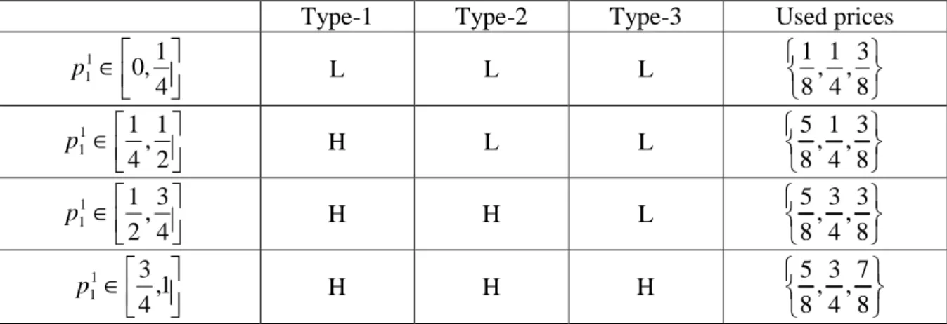
The objective of the boss is to minimize the expected loss caused by bounded rationality. He can send four different kinds of reports to his namesake. These reports and their corresponding perceived categories for each type are given in Table 1. For example, if the boss chooses to report a price in [0,1/2], then all the types consider their low categories, and use 1/8, 1/4, 3/8 as representative, respectively.

Table 1 - Action Space

Type-1 Type-2 Type-3 Used prices

      ∈ 4 1 , 0 1 1 p L L L       8 3 , 4 1 , 8 1       ∈ 2 1 , 4 1 1 1 p H L L       8 3 , 4 1 , 8 5       ∈ 4 3 , 2 1 1 1 p H H L       8 3 , 4 3 , 8 5       ∈ ,1 4 3 1 1 p H H H       8 7 , 4 3 , 8 5

We consider a myopic approach in this section. That is, we assume that the boss is only concerned with the expected loss of the current period, not with the aggregate expected loss. A farsighted approach is considered in the following section. Table 2 shows the expected loss for each possible combination of price realizations on the first market ( ) and actions taken by the boss.

Each number in bold gives the minimum expected loss for the relevant price realization. Under the myopic approach, the action that corresponds to each bold number is optimal for the relevant price realization. For example, if the boss observes a price on the first market that belongs to interval [0,1/8], he will report a price that belongs to interval [0,1/4]. At this point we make another assumption about the boss. We assume that he prefers to tell the truth whenever it is among the optimal actions. This assumption together with the fact that [0,1/8]⊂[0,1/4] (truth-telling is among optimal actions) imply that the boss reports the observed value in this case. However, if [1/4,3/8] it is optimal to report [0,1/4]. In this case, the reported price is less than the observed value (the boss under-states the price). The other case in which the boss lies is when [5/8,3/4]. The optimal action of the boss, in this case, is to report [3/4,1], i.e., he reports a price that is higher than the observed value (the boss over-states the price).

Table 2 - Expected Loss (common multiplier: ₃ 8 6 1 × ) Observed Price \ Report ∈ 1 p [0,1/4] p1∈ [1/4,1/2] p1∈ [1/2,3/4] p1∈ [3/4,1] ∈ 1 1 p [0,1/8] 9 29 57 93 ∈ 1 1 p [1/8,1/4] 3 15 35 63 ∈ 1 1 p [1/4,3/8] 3 7 19 39 ∈ 1 1 p [3/8,1/2] 9 5 9 21 ∈ 1 1 p [1/2,5/8] 21 9 5 9 ∈ 1 1 p [5/8,3/4] 39 19 7 3 ∈ 1 1 p [3/4,7/8] 63 35 15 3 ∈ 1 1 p [7/8,1] 93 57 29 9

From Table 2 we obtain the following reaction function:              ∈     ∈     ∈     ∈ = . , 4 3 , 48 5 1 , 4 3 , 8 3 , 4 1 4 1 , 0 ) ( 1 ₁1 1 1 1 1 1 otherwise price true report p if p report p if p report p R (1)

Under-statement occurs only if [1/4,3/8] and receiving this report all types use their low (L) categories (see Table 1). However, if [1/4,3/8] and the boss reports the true value of the price rather than under-stating, type-1 uses his high (H) category whereas type-2 and 3 stick to their low (L) categories. So, it is only type-1 who is affected by under-statement. Since the boss prefers to tell the truth whenever it is among the optimal actions and under-statement does not affect other types, the boss uses this strategy only if type-1 is among possible types when the observed price belongs to interval [1/4,3/8].

Over-statement occurs only if [5/8,3/4]. By the same reasoning as above, over-statement affects only type-3, not others. Therefore, the boss uses this strategy only if type-3 is among possible types when [5/8,3/4]. Otherwise, he prefers to report the truth.

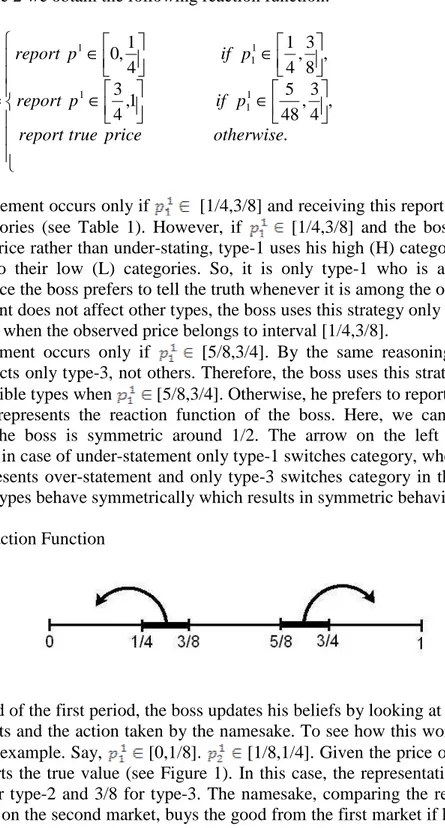
Figure 1 represents the reaction function of the boss. Here, we can observe that the behavior of the boss is symmetric around 1/2. The arrow on the left represents under-statement and in case of under-under-statement only type-1 switches category, whereas the arrow on the right represents over-statement and only type-3 switches category in this case. As noted earlier, these types behave symmetrically which results in symmetric behavior of the boss. Figure 1 - Reaction Function

At the end of the first period, the boss updates his beliefs by looking at the prices realized in both markets and the action taken by the namesake. To see how this works let us consider the following example. Say, [0,1/8]. [1/8,1/4]. Given the price on the first market, the boss reports the true value (see Figure 1). In this case, the representative price is 1/8 for type-1, 1/4 for type-2 and 3/8 for type-3. The namesake, comparing the representative price with the price on the second market, buys the good from the first market if he is of type-1 and buys from the second market otherwise. In such a situation, the namesake's action reveals whether he is of type-1 or not, and the boss updates his belief accordingly.

Figure 2 summarizes the learning process at the end of period-1. Numbers in bold stand for the numbers of possible types of the namesake. The boss starts with three possible and equally likely types. The probability that he learns the exact type, i.e., that the number for possible types reduces to 1, at the end of the first period is 3/32=0.09375. The probability that the number of possible types decreases to 2 (elimination of one type) is 3/16=0.1875, and finally the probability that the boss learns nothing is 23/32=0.71875.

Figure 2 - Learning Process, 1st Period

The boss starts the second period with updated beliefs. The objective is again to minimize the expected loss caused by bounded rationality. When type-1 is among possible types and the observed price on the first market in the second period ( ) belongs to the interval [1/4,3/8], he uses the under-statement strategy described above. Furthermore, when type-3 is among possible types and [5/8,3/4], he uses the over-statement strategy. In all the other cases he reports the true observed value. The reaction function for the second period coincides with the one for the first period (Figure 1) if both type-1 and type-3 are among possible types.

Figure 3 summarizes the learning process for the whole game. If the boss figures out the exact type of the namesake (arrives to node 1) at the end of the first period, there is nothing left to learn and he continues the second period with the relevant strategy. If he arrives to node 2 at the end of the first period, the learning process continues and he might either figure out the type and arrive to node 1 or not learn anything new and stay in node 2. If, at the end of the first period, he does not learn anything about the type (stays at node 3), there are three possibilities for the second period. He might figure out the exact type and arrive to node 1, or he might eliminate only one possible type and arrive to node 2, or he might not learn anything and stay at node 3. The overall probability that the boss figures out the exact type of the namesake by the end of the game is 0.19238, that he eliminates only one possible type is 0.29102 and that he does not learn anything is 0.51660.

Figure 3 - Learning Process, 2nd Period

The transition matrix of the learning process is given in Table 3. It is a finite Markov Chain and has three ergodic states. According to the Theorem by Kemeny and Snell (1976), the probability after n steps that the process is in an ergodic state tends to 1, as n tend to infinity. This means that if the game is repeated for n periods the probability that the boss learns the exact type of the namesake tends to 1 as n gets larger.

Table 2 - Transition Matrix possible types {1,2,3} {1,2} {1,3} {2,3} {1} {2} {3} {1,2,3} 0.71875 0.08333 0.02083 0.08333 0.04167 0.01042 0.04167 {1,2} 0 0.84375 0 0 0.07813 0.07813 0 {1,3} 0 0 0.75000 0 0.12500 0 0.12500 {2,3} 0 0 0 0.84375 0 0.07813 0.07813 {1} 0 0 0 0 1 0 0 {2} 0 0 0 0 0 1 0 {3} 0 0 0 0 0 0 1

The relationship between the number of periods and the probability of learning the exact type is given in Table 4. The probability increases in the number of periods, and it becomes almost 1 after 30 periods.

Table 3 - Number of periods/probability

n p 5 0.46344 7 0.60419 10 0.75543 15 0.89388 20 0.95465 30 0.99178

A crucial point to be noted is that in this section we use a myopic approach to solve the optimization problem. The boss is concerned only with the expected loss of the period he is in, whereas under a farsighted approach, he considers the overall expected loss that is the sum of discounted future expected losses. However, both approaches yield the same results with the given available types. It follows from the fact that a manipulated message affects only one type, while other types stick to their category that they would consider if the message was not manipulated. In other words, a strategy that needs to be used in order to decrease the expected loss caused by one type does not conflict with the strategies that need to be used for other types. For example, the under-statement strategy is used whenever type-1 is among possible types. The fact that type-2 and/or type-3 are among possible types does not change this strategy, because it induces only type-1 to change his category, not the other types. Therefore, the boss can continue to use the reaction function given in Figure 1 even if he knows the exact type of the namesake. It should be noted that if he does so, he might report a manipulated price although reporting the true value is also among optimal actions. Even though this violates our assumption that the boss prefers truth telling whenever it is possible, it yields the same expected loss for the boss. This fact ensures that he can use the same reaction function for each period no matter if he is farsighted or myopic. In the following section we show that myopic and farsighted optimizations do not always coincide.

3. Farsighted Approach

In this section, we consider a farsighted approach and assume that the objective of the boss is to minimize the sum of discounted expected losses. We modify the model by changing the possible types. Here, we assume that the namesake has two possible types. The first type uses two categories (low and high) and his cutoff price level is 1/3. Therefore he uses 1/6 as the representative for low category (L) and 2/3 for high category (H). The second type uses three categories (low, medium and high) and his cutoff price levels are 1/3 and 2/3. Thus 1/6, 1/2 and 5/6 are the representative prices for his low (L), medium (M), and high (H) categories, respectively. The prior belief of the boss is that both types are equally likely.

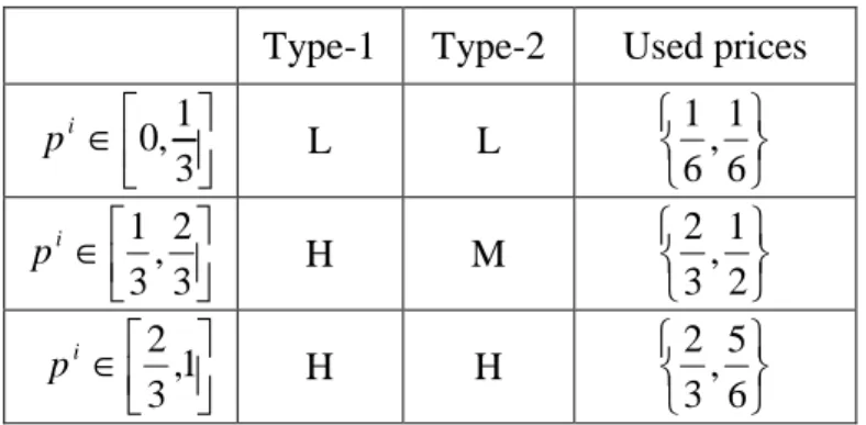
In this setting, the boss can choose his strategy among three different types of action, which are represented in Table 5. If he reports a price belonging to [0,1/3], both types use low categories and 1/6 as representative price. If he reports [1/3,2/3], then type-1 uses his high category and 2/3 as his representative for the first market price, and type-2 uses his medium category and 1/2 as the representative (i∈{1,2}represents the period). Finally, if the boss reports [2/3,1], both types will use high categories and type-1 uses 2/3 whereas type-2 uses 5/6 as representative price.

Table 4 - Action Space

Type-1 Type-2 Used prices

      ∈ 3 1 , 0 i p L L       6 1 , 6 1       ∈ 3 2 , 3 1 i p H M       2 1 , 3 2       ∈ ,1 3 2 i p H H       6 5 , 3 2

We solve the optimization problem by backward induction. If the boss does not learn anything about the type of his namesake during the first period, he starts the second period with the belief that both types are equally likely. Following the same reasoning of the previous section, we get the following reaction function:

        ∈     ∈ = , , 60 23 , 3 1 3 1 , 0 ) 2 & 1 | ( 2 1 2 2 1 otherwise price true report p if p report type type p R (2)

where R(p12|type1 &type2) stands for the reaction function for the second period given that both type-1 and type-2 are among possible types. And the expected loss in this case is

. 17280 151 ) 2 & 1 | ( 2 L type type = E (3)

If the boss learns that his namesake is of type-1 during the first period, his reaction function for the second period is

        ∈     ∈ = , , 60 25 , 3 1 3 1 , 0 ) 1 | ( 2 1 2 2 1 otherwise price true report p if p report type p R (4)

and the expected loss in this case is

. 576 7 ) 1 | ( 2 L type = E (5)

Finally, if the boss starts the second period with the information that his namesake is of type-2, his reaction function in this period is to always report the true value. This follows from the fact that this type uses optimal categorization given the number of categories and the distribution of the price. In this case, the expected loss is

. 216 1 ) 2 | ( 2 L type = E (6)

Now, we move to the first period. If the boss, after observing the price on the first market, reports [0,1/3] then both types use low category and 1/6 as representative price for the first market (see Table 5). Therefore, it is impossible for the boss to distinguish between the two types. In this case, the overall expected loss is

(7)

where

δ

If the boss reports [1/3,2/3] then type-1 uses his high category and 2/3 as representative price for the first market, whereas type-2 uses his medium category and 1/2 as representative (see Table 5). In such a case, both types act in the same way conditional on the price realization of the second market being either lower than 1/2 or greater than 2/3. In the former case they both buy from the second, whereas in the latter case they buy from the first market. The two types take diverse actions only if [1/2,2/3]; type-1 buys from the second and type-2 buys from the first market. Hence, with this strategy the probability that he boss figures out the type of his namesake is 1/6 and his expected loss is

(8)

Finally, if the reported price is such that [2/3,1] then both types consider their high category and use 2/3 and 5/6 as representative price, respectively (see Table 5). In this case,

the two types take different actions only if the price realization on the second market belongs to [2/3,5/6], which occurs with probability 1/6. Hence, the expected loss in this case is

(9)

Inserting (3), (5) and (6) into (7), (8) and (9) we derive the reaction function of the boss as follows:

[ ]

Taking into account the assumption that the boss prefers to tell the truth whenever possible, the above reaction function becomes

        ∈     ∈ = . , , 3 1 3 1 , 0 ) ( 1 1 1 1 1 otherwise price true report a p if p report p R (10)

The reaction function (10) depends on the discount factor . This implies that the optimal strategy of the boss when he is myopic ( =0) is different than when he is farsighted ( >0). This follows from the fact that a farsighted boss wants to invest in learning the type since he is concerned with his future losses as well as the current one. The difference here is quite small because the game we consider has only two periods. When the number of periods increases, not only the occasions in which he can learn about his namesake but also the value of knowing the type grows for a farsighted boss. As a result, the difference becomes important.

4. Conclusion

We have constructed a model in order to study the interaction between fully and boundedly rational agents when they are in a team and have perfectly aligned preferences. In an environment with abundance of product information (type, quality, brand, age of the good, length of the warranty, payment arrangements and service fees), boundedly rational agents are having difficulties in making decision due to their cognitive limitations. In order to simplify the situation, they try to group events, objects or numbers into categories. In our model we consider a boundedly rational agent who partitions the price space into connected sets. The decision made by this agent might be non-optimal in some cases, since he is using categories instead of realized prices and regards prices belonging to the same category as equal.

Assuming different types for the boundedly rational agent that differ in categories used, we show that during his interaction, the fully rational agent may learn about the type of the boundedly rational agent. He can improve the outcome by using this additional information. The probability that he learns the type of the boundedly rational agent increases in the length of this interaction, whereas it decreases in the number of available types.

Finally, we show that myopic and farsighted approaches yield different results, depending on the available types. This difference is caused by the tradeoff between investing in learning the agent's type with the aim of decreasing future losses and minimizing the current period's expected loss.

References

Allport, G.W. (1954). The Nature of Prejudice. Reading, MA: Addison Wesley.

Chen, Y., Iyer G. & Pazgal A. (2010). Limited Memory, Categorization, and Competition. Marketing Science, 29(4), 650-670.

Crawford, V. & Sobel J. (1982). Strategic Information Transmission. Econometrica, 50, 1431-1451.

Dow, J. (1991). Search Decisions with Limited Memory. Review of Economic Studies, 58, 1-14.

Eliaz, K. & Spiegler R. (2006). Contracting with Diversely Naive Agents. Review of Economic Studies, 73(3), 689-714.

Fryer, R. & Jackson M. O. (2008). A Categorical Model of Cognition and Biased Decision Making. The B.E. Journal of Theoretical Economics, Vol. 8: Iss. 1 (Contributions), Article 6.

Hong, L. & Page S. (2009). Interpreted and Generated Signals. Journal of Economic Theory, 144, 2174-2196.

Kemeny, J. G. & Snell J. L. (1976). Finite Markov chains. New York: Springer-Verlag. Luppi, B. (2006). Price Competition over Boundedly Rational Agents, mimeo.

Macrae, N. & Bodenhausen G. (2000). Social Cognition: Thinking Categorically About Others. Annual Review of Psychology, 51, 93-120.

Piccione, M. & Rubinstein, A. (2003). Modeling the Economic Interaction of Agents with Diverse Abilities to Recognize Equilibrium Patterns. Journal of European Economic Association, 1, 212-223.

Radner, R. (1962). Team Decision Problems. Annals of Mathematical Statistics, 33, 857-881. Rosch, E. & Mervis C. B. (1975). Family resemblances: Studies in the Internal Structure of

Categories. Cognitive Psychology, 7, 573-605.

Rubinstein, A. (1993). On Price Recognition and Computational Complexity in a Monopolistic Model. Journal of Political Economy, 101, 473-484.

Simon, H. A. (1987). Bounded Rationality. In The New Palgrave: A Dictionary of Economics, Vol. 1, eds. J. Eatwell, M. Milgate, P. Newman, 266-286. London: MacMillan.

Tversky, A., & Kahneman D. (1981). The Framing of Decision and the Psychology of Choice. Science, 211, 453-458.