Sensitivity analysis of directivity effects on PSHA
E. ChioCCarElliand i. iErvolinoDipartimento di Ingegneria Strutturale, Università Federico II, Napoli, Italy (Received: June 11, 2011; accepted: April 16, 2013)
ABSTRACT Careful characterization of seismic hazard is especially important in structural
engineering if critical facilities (e.g., strategic buildings, chemical deposits, energy production plants, etc.) are the object of analysis. Moreover, if the construction site is close to active faults, particular attention is required. In fact, in this condition, the fault’s dynamics affect ground motion differently from site to site, resulting in systematic spatial variability, and, generally, in higher seismic demand, with respect to the far-source case. The most important of the near-source (NS) effects is known as forward rupture directivity, and can be identified by a large full-cycle pulse at the beginning of the velocity records, and containing the most of carried energy. Recent research demonstrates that, from the structural engineering point of view, hazard assessment should account for NS effects (i.e., pulse-like ground motions), but ordinary probabilistic seismic hazard analysis (PSHA) is not able to do it appropriately. On the other hand, semi-empirical models calibrated for introducing NS effects in classical PSHA are now available, and some preliminary attempts of numerical implementation of NS-PSHA exist. In the presented study, numerical applications of strike-slip (SS) fault scenarios are provided and, for a fixed return period, uniform hazard spectra are computed in order to quantify hazard increments (HIs) due to NS-PSHA with respect to ordinary-PSHA. It is shown that: i) depending on source-site geometry, these may be significant (more than a 100% increment); ii) different spectral periods are affected by significantly different values of HIs, which have their shape controlled only by the magnitude of generated earthquakes; iii) it is possible to identify a zone beyond which directivity effects are expected to become negligible, at least with a first-order approximation, independently of the characteristics of the considered SS fault.
Key words: hazard increments, pulse-like records, near-fault, fault scenario.
1. Introduction In near-source (NS) conditions, ground motions and seismic structural response, may show spatial variability systematically different from what shown in far-source condition. This is mainly because of rupture’s forward directivity, which may most likely affect near-fault sites in particular geometrical configurations with respect to the rupture. The resulting phenomenon, of largest engineering interest, is a large full-cycle pulse at the beginning of velocity record
containing most of its energy, and mainly observed in fault-normal (FN) component (Somerville et al., 1997)1.
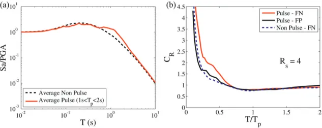
A discussion of directivity effects was given with respect to the recent L’Aquila 2009 (central Italy) earthquake (moment magnitude equal to 6.3), and a detailed analysis can be found in Chioccarelli and Iervolino (2010). In this same study, analyzing a large American data set [next generation attenuation (NGA) database, http://peer.berkeley.edu/nga/ (last access June 2013)], three main features of engineering interest characterizing pulse-like records, if compared to those non-pulse-like (hereafter referred to as ordinary), were found: 1) pulse-like signals are characterized by FN components generally stronger than fault parallel (FP) (non-pulse-like ground motions have equivalent median FN and FP components); 2) FN pulse-like signals are characterized by a non-standard spectral shape with an increment of spectral ordinates in a range around the pulse period (Tp); 3) the CR factor, defined as the ratio between inelastic spectral displacements [of a single degree of freedom (SDoF) system with given strength reduction factor, RS] to the corresponding elastic spectral displacement, can be, for FN pulse-like records, 20% ÷ 70% larger than that of ordinary motions, depending on the non-linearity level (see also Iervolino et al., 2012). Such increments are displayed in a range of periods between about 30% and 50% of pulse period. This is especially relevant for earthquake resistant structural design and assessment. An analysis of inelastic displacement demand associated to forward-directivity ground-motions is also provided in Ruiz-Garcìa (2011).
In Fig. 1a, the average of the FN elastic spectra, normalized to peak ground acceleration (PGA) is given for pulse-like records considered herein, with Tp between 1 and 2 s (Average Pulse), and for ordinary ground motions (Average Non Pulse), both taken from NGA. In Fig. 1b, referring to the same database, CR for an RS = 4 is given for pulse-like and non-pulse-like records (Pulse - FN and Non Pulse - FN, respectively). The figures allow the appreciation of the systematic differences summarized above, especially points 2) and 3), among the considered classes2. Moreover, C
R for the FP components of the pulse-like FN records (which not
necessarily are pulse-like, even if indicated as Pulse - FP), is shown: it appears that FP records have a shape similar to FN in the low T/Tp range, yet with lower amplitudes.
Identification of design seismic actions is a fundamental step in the assessment of structural seismic risk and the most consolidated framework to deal with this issue is the probabilistic seismic hazard analysis (PSHA) (Cornell, 1968; McGuire, 2004): it allows to build hazard curves for selected ground motion intensity measures (IMs), starting from seismic source models and ground motion prediction equations (GMPEs). However, it has been formulated for ordinary conditions and needs adjustments for sites close to a seismic fault and, then, potentially subjected to pulse-like directivity effects. Therefore, because ordinary PSHA is adopted by most advanced seismic codes worldwide (e.g., CEN, 2003; C.S.LL.PP., 2008), such codes provide design actions with respect to which directivity may represent an unexpected demand. This seems especially important in the case of critical structures. On the other hand, NS-PSHA 1 Generally, in seismology the term directivity is used to indicate the azimuthal variation of the radiated seismic energy due to the geometry of the rupture growth (Boatwright and Boore, 1982). In this study, the term directivity is referred to the physical phenomena producing pulse-like ground motions.
2 A T
P can be assigned also to ordinary records (even if non-significant), rendering possible a representation as a
Fig. 1 - a) Elastic 5% damped spectra for FN pulse-like with 1 s < Tp < 2 s and ordinary records; b) empirical CR for FN pulse-like records, for their FP components, and for ordinary records, at RS = 4. Figure adapted from Iervolino et al. (2012). requires an increased computational effort because, as shown in the following, additional random variables are involved with respect to the classical case. The aim of this work is to provide quantification of directivity effects in hazard assessment if compared to ordinary analysis, together with some preliminary indications about the geographic area around a strike-slip (SS) fault in which significant directivity effects should be expected. The paper is structured so that modified PSHA accounting for pulse-like issues is presented first, recalling all the necessary models already available in literature. Then, some illustrative applications are carried out3; results of ordinary and modified PSHA are compared referring
to a fixed return period of seismic action. Selecting a specific site, analyses of the whole pseudo-acceleration uniform hazard spectra (UHS) are shown, discussing trends of hazard increments (HIs) of NS - with respect to ordinary - PSHA. Moreover, directivity effects in the area around the fault are analyzed showing that, with a significant reduction of computational effort, a quantitative estimation of HIs in each site can be provided. Although results refer to the presented applications, trends expected to be systematic can be identified.
2. Modified PSHA for near-source conditions
As mentioned, ordinary PSHA cannot account for spatial ground motion variability, which may affect NS sites. More specifically, the two main limits can be found in the GMPEs, and in the identification of relative site-source configuration. In fact, ordinary GMPEs are fitted on ground motion databases in which pulse-like records, if any, are usually scarce, and often rotated differently to FN and FP directions. Moreover, because each record is characterized by a different 3 All of them refer to single fault scenarios because NS-PSHA requires the knowledge of size and location of the rupture, and cannot be directly applied using seismic source zones (e.g., Meletti et al., 2008). However, if critical facilities are of concern, it is reasonable to imagine a deeper knowledge of seismic faults in the building area.
Tp, the influence of pulse-like spectral shape on such GMPEs is masked and/or spread over a broad range of periods (Shahi and Baker, 2011). On the other hand, not all NS sites are equally prone to be subjected to directivity effects (Somerville et al., 1997; Iervolino and Cornell, 2008) and the simple source-to-site distance, used in ordinary PSHA, is not enough to identify where probability of pulse-like records is larger.
Recent attempts in solving these issues were aimed at retaining the general PSHA framework, introducing some directivity-related adjustments (e.g., Abrahamson, 2000; Tothong et al., 2007; Iervolino and Cornell, 2008). All required probabilistic models are available nowadays, and preliminary applications may be found in Chioccarelli (2010) and Shahi and Baker (2011).
Herein, in order to describe the modified procedure, the standard approach to PSHA is first recalled. Assuming a homogenous Poisson model of earthquake occurrence, Eq. (1) is used for computing the mean annual frequency (MAF, or PSHA
IM
λ ) of exceeding a ground motion intensity
measure threshold, in the case a single seismic source is considered. Hereafter, the chosen IM is the elastic spectral acceleration (Sa) at a fixed period T, that is Sa(T). M is the magnitude of the earthquake (hereafter moment magnitude) and R is the source-to-site distance, ν is the mean annual rate of earthquakes occurrence on the source within a magnitude range of interest, fM, R is the joint probability density function (PDF) of M and R. Finally GSa|M, R is the complementary cumulative distribution function (CCDF) of Sa (usually lognormal, if obtained by a GMPE).
λ PSHA
(
S a)
= ν ·�
m�
r GSa | M, R(
Sa |m, r)
· fM, R(
m, r)
· dm · dr (1) Sa NS-PSHA considers the MAF(
NS PSHA)
Sa λ − to be a linear combination of two hazard termswhich account for the absence or the occurrence of the pulse, λSa,NoPulse and λSa,Pulse respectively, as reported in Eq. (2).
. (2)
The two terms of Eq. (2) are implicitly weighted by the pulse occurrence probability, P[Pulse|Z], which is provided by Iervolino and Cornell (2008).4 The latter, in fact, depends
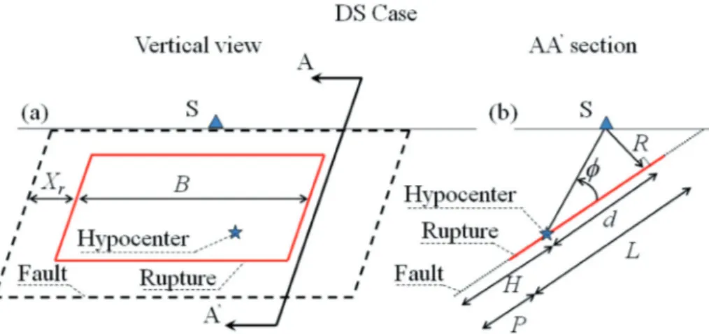
on the relative source-site configuration, which is identified by simple geometrical parameters represented by the Z vector of variables. Such variables are known once rupture, hypocentre, and site positions are known. In the case of SS rupture (Fig. 2a), Z is comprised of rupture-to-site distance (R), the distance from the epicenter to the site measured along the rupture direction (s), and angle between the fault strike and the path from epicenter to the site (θ). It should be noted that the probability model in Iervolino and Cornell (2008) is defined for R, s and θ varying in the intervals of (0 - 30 km), (0 - 40 km) and (0° - 90°), respectively. In the applications to follow, zero pulse probabilities are associated to values outside the covariates’ intervals where model applies.
Two other issues, which are not faced in traditional hazard analysis, appear in NS-PSHA: i) pulse period prediction; ii) pulse amplitude prediction.
( )
,( )
,( )
NS PSHA
Sa sa Sa NoPulse sa Sa Pulse sa
λ − =λ +λ
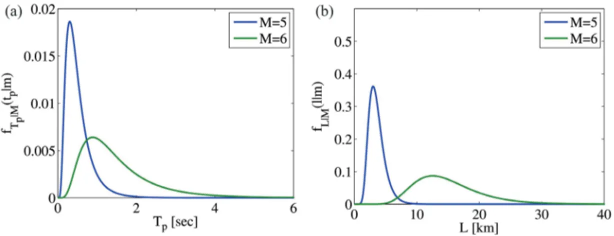
The former (i) has been addressed by many authors referring to a lognormal random variable conditional on the event magnitude; i.e., fTp|M (tp|m), the parameters of which were retrieved on an empirical basis. The model considered herein is from Chioccarelli and Iervolino (2010) (Fig. 2b), but others are available; see Tang and Zhang (2010) for a review.
The latter issue (ii) should be accounted for fitting a new GMPE on pulse-like records generated by rupture directivity effects only. Alternatively, an easier procedure was proposed by Baker (2008) referring to the already available ordinary GMPE of Boore and Atkinson (2008) and modifying it in order to be representative of pulse-like spectra. Thus, the modification factor, operating on the mean value of logarithms of spectral pseudo-acceleration, is a function of Tp as shown in Eq. (3). It consists of adding a ‘bump’ of spectral ordinates around the pulse period. In the equation, ln
(
Sa(T))
is the expected value of logarithms of spectral acceleration predicted by the original GMPE (GSa in the following), and ln(
Sa,mod (T))
is the value provided by modified GMPE (GSa,mod). . (3) Eqs. (4) and (5), expand Eq. (2) in the case of a single fault with SS style. In numerical applications of this rupture case (to follow), the geometrical parameters required by pulse occurrence probability model are transformed in the rupture length (L), the position of the rupture on the fault (P), and the epicenter location (E), as reported in Fig. 2a. A deterministic relationship between these parameters and {R, s, θ} vector exists. Thus, the Z vector can be replaced by a vector comprised of L, P and E. This allows to more easily simulate the uncertainty involved for hazard computations, that is, distributions can be conveniently assigned for {L, P, E}, then {R, s, θ} may be retrieved and pulse occurrence probability can be calculated: (4) Fig. 2 - SS geometrical parameters in plan (a) and regression model for TP (b).( )
(
)
(
)
( )
( )
, , , , , , , , , = ⋅ ⋅ ⋅ ⋅ ⋅ ⋅ ⋅ ⋅ ⋅∫ ∫ ∫ ∫
Sa NoPulse a Sa M L P a m l p e M P E L L M s P NoPulse l p e G s m l p f p e l f l m f m dm dl dp de λ ν(5)
.
In Eqs. (4) and (5) statistical dependencies are explicitly indicated for all the distributions already introduced; indeed, fP, E|L (p, e|l) is the uniform distribution of P and E on the rupture length, fL|M (l|m) is the distribution of L on the event magnitude [provided by Wells and Coppersmith (1994)], fM (m) is the model of magnitude distribution.
Eq. (4) refers to the case of pulse absence: ordinary5 GMPE depending on geometrical
parameters (L and P) is used6, G
Sa|M,L,P, and results are weighted for the corresponding pulse
absence probability, P [NoPulse|l, p, e] = 1 – P [Pulse|l, p, e]. All the other terms are equal to those of Eq. (1), in which pulse-like effects are not considered. Conversely, Eq. (5) refers to the case of pulse occurrence as indicated by the pulse occurrence probability P [Pulse|l, p, e] and by the modified GMPE, GSa,mod|Tp,M,L,P, in which the additional dependency on Tp, fTp|M (tp|m), has to be considered to model the spectral increments around the pulse period according to Eq. (3). Further details on the terms appearing in the equations and not shared by classical PSHA can be found in Chioccarelli and Iervolino (2013).
2.1. NS-PSHA for dip-slip faulting style
Eqs. (4) and (5) can also be written for dip-slip (DS) ruptures. The general framework and numerical procedure are not significantly different from what already shown. In fact, Eq. (2) and all the models introduced in the previous section can be applied; however, minor differences can be identified; they are due to the different geometrical configuration of DS ruptures with respect to SS. More specifically, at least with respect to the issues addressed in this work, DS ruptures cannot be represented by a bi-dimensional scheme (as for the SS case in Fig. 2a), thus (at least) one additional random variable has to be introduced. In Fig. 3 two orthogonal sections of DS rupture are represented assuming the hypothesis of rectangular fault and rectangular rupture.
Eqs. (6) and (7) can be used for DS case considering the following differences with respect to Eqs. (4) and (5):(4) and (5):
1) position of the epicentre, E, has to be replaced by the position of the hypocentre (H); 2) the rupture’s geometrical parameter dependent on event magnitude is assumed to be the
rupture length L, in analogy with the SS case (in principle it should be the area of the rupture from which B and L depend); moreover, the B/L ratio is assumed to be constant for the sake of simplicity;
3) to compute pulse occurrence probability, rupture location within the fault (Xr) is required (for computation of R, along L, P, and H); it is the additional random variable;
4) the introduction of Xr requires knowledge of its PDF conditional to L, fXr|L (xr|l):
( )
(
)
(
)
(
)
( )
( )
, ,mod , , , , , , , , , , = ⋅ ⋅ ⋅ ⋅ ⋅ ⋅ ⋅ ⋅ ⋅ ⋅ ⋅∫ ∫ ∫ ∫ ∫
p p p Sa Pulse a Sa T M L P a p t m l p e p M p T M P E L L M s P Pulse l p e G s t m l p f t m f p e l f l m f m dt dm dl dp de λ ν5 As explained, percentage of pulse-like records in ground motions databases and heterogeneity of pulse periods suggest that directivity effects may be neglected in ordinary GMPEs and the latter can be used for non-pulse hazard contribution. However, a deamplification factor of mean (Sa) predicted by the GMPE of Boore and Atkinson (2008)
was recently proposed Shahi and Baker (2011) in the (0 - 10 km) range of Rjb (i.e., Joyner and Boore, 1981) distance
and for magnitude higher than 6.0. In the same paper, no corrections are suggested for standard deviation of considered GMPE model.
6 If R
(6)
(7)
.
In Chioccarelli and Iervolino (2013) it is shown that numerical results of SS and DS cases have similar general trends independently on the specific rupture mechanism. Thus in the following, SS ruptures are considered for simplicity.
( )
(
)
(
)
(
)
(
)
( )
, , , , , , , , , , , , r r r Sa NoPulse a r Sa M X L P a r m l p h x r M r P H L X L L M s P NoPulse l p h x G s m l p x f p h l f x l f l m f m dm dl dp dh dx λ =ν⋅ ⋅ ⋅ ⋅ ⋅ ⋅ ⋅ ⋅ ⋅ ⋅ ⋅∫ ∫ ∫ ∫ ∫
( )
(
)
(
)
(
)
(
)
(
)
( )
, ,mod , , , , , , , , , , , , , p r p r p r Sa Pulse a r Sa T M X L P a p r t m l p h x p r M p r T M P H L X L L M s P Pulse l p h x G s t m l p x f t m f p h l f x l f l m f m dt dm dl dp dh dx λ =ν⋅ ⋅ ⋅ ⋅ ⋅ ⋅ ⋅ ⋅ ⋅ ⋅ ⋅ ⋅ ⋅∫ ∫ ∫ ∫ ∫ ∫
Fig. 3 - DS rupture representations through two vertical and mutually orthogonal sections.
3. Illustrative applications
Preliminary analyses of directivity effects in terms of spectral response were provided by cited studies (i.e., Chioccarelli, 2010; Shahi and Baker, 2011; Chioccarelli and Iervolino, 2013), which address HIs due to NS-PSHA with respect to the ordinary one. Results therein show that numerical values of such increments are dependent on geometrical parameters determining the source-to-site configuration, such as fault dimensions and site location. In order to deepen this issue, additional illustrative applications are presented here retaining the hypothesis of known fault geometry, which is common to all the previous works regarding this topic. In fact, the results’ sensitivity to uncertainties related to the fault is not discussed here, although believed to be relevant. As shown in Eqs. (4) and (5), rupture length and rupture position are, in principle, random variables: the former can be assumed lognormal conditional on the event magnitude (Wells and Coppersmith, 1994) and the latter uniformly distributed on the fault. However, applications are
here implemented in the simplifying hypothesis of fixed rupture dimension and position. Such hypothesis appears to be acceptable if a single magnitude can be generated by the considered fault (as assumed in the following). The hypothesis of uniform distribution of the epicenter position on the rupture is retained.
Two cases of single generated magnitude, equal to 5.0 and 6.0, are considered. In Fig. 4a, PDF of Tp (Chioccarelli and Iervolino, 2010) is reported for the two fixed values of magnitude because, as shown in the following section, results are strongly dependent on such distributions.
Starting from the Wells and Coppersmith (1994) prediction model which assumes a lognormal distribution (base 10) of rupture dimension (Fig. 4b), two fixed source length are associated to each magnitude scenario. More specifically, fifth and fiftieth percentiles of rupture length distributions are chosen: 2.0 and 3.4 km SS lengths are associated to M 5.0, while 8 and 14 km are obtained for the M 6.0 scenarios.
In the following, seismic hazard is estimated via the uniform hazard spectrum for a return period (Tr) equal to 475 years; used GMPE is that of Boore and Atkinson (2008); mean annual rate of earthquake occurrence on the fault is 0.05. Attention is focused on HIs if ordinary PSHA is replaced by its modified version for NS sites. In most of the advanced seismic codes worldwide (e.g., CEN, 2003; C.S.LL.PP., 2008), the seismic threat is characterized by UHS computed by ordinary PSHA and quantification of HIs in NS conditions is useful to understand the consequences of neglecting pulse-like directivity effects in hazard analysis. For each spectral period T and for the chosen Tr = 475, hazard increments HI (T) are analytically defined by the percentage factor in Eq. (8):
Sa (T)NS–PSHA – Sa (T)PSHA
HI (T) = ––––––––––––––––––––– · 100 (8)
Sa (T)PSHA
Analyses of a specific site is reported first (Section 3.1), then, contours of HI (T) in the area around the seismic sources are studied for single spectral periods (Section 3.2). This is in order to extend previous site-specific results to a wider area. In fact, contours are also useful
for identification of the distance from the fault beyond which NS-PSHA provides negligible differences with respect to PSHA.
3.1. Analysis of spectral pulse-like effects for a specific site
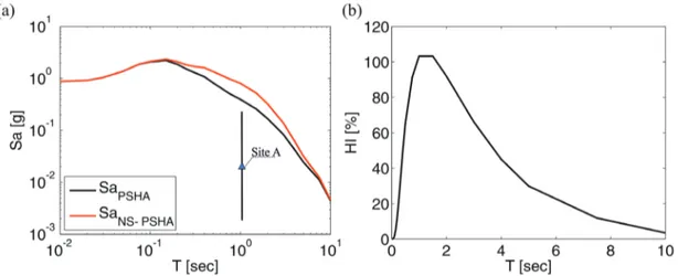
A 8 km SS fault is considered with a M 6.0 associated to all generated events (Fig. 5a). UHS are computed with ordinary and modified PSHA for the site in the middle of the fault (site A) where the influence of directivity effects was checked to be the largest (Chioccarelli and Iervolino, 2011; Shahi and Baker, 2011; Chioccarelli and Iervolino, 2013). Pseudo-acceleration response spectra are reported in Fig. 5a while HI (T) are shown in Fig. 5b. As expected, the shape of increments is strictly related to the prediction model of pulse periods (Chioccarelli and Iervolino, 2010) (Fig. 4a) and maximum increments (larger than 100%) affect a range of periods around the median of Tp distribution for M 6.0 (equal to 1.3 s). Conversely, structural periods far from 1.3 s are interested by lower values of HI (T).
Assuming a 2 km SS fault capable of generating M 5 events, UHS and HIs are computed for the site in the middle of the fault (as per the previous case) and are reported in Figs. 6a and 6b, respectively. Again, maximum hazard increments are in accordance with median value of predicted Tp for M 5.0 (Fig. 4a), which is equal to 0.43 s.
It is interesting to note that, in both cases, maximum values of HI (T) are about 100% (107% and 102% for M 5.0 and M 6.0, respectively) which means that NS-PSHA induces actions twice as large than the PSHA in these case-studies. It suggests that, independently on the absolute value of spectral accelerations and on the magnitude of generated events, similar geometrical location of the site on the fault determines similar maximum numerical HI (T). This issue will be verified in Section 3.2. In both cases, spectral periods interested by maximum HI (T) are closely related to the Tp prediction model (see Fig. 4a), which is dependent on the event magnitude only. This suggests that the fault’s characterization, in terms of generated magnitudes, can be used for the prediction of most dangerous range of periods which results from NS-PSHA [see Chioccarelli and Iervolino (2010) and Ruiz-Garcìa (2011) for details about the relationship betweenRuiz-Garcìa (2011) for details about the relationship between for details about the relationship between Tp, T, and inelastic structural demand].
3.2. Pulse-like-prone near-source areas
In this section the analysis of hazard increments is extended to the whole area affected by the considered sources. UHS and HIs were computed for 64 sites influenced by the 8 km SS fault. Studied sites were identified by a 5 by 10 km lattice over a 40 by 60 km area. Results, not shown herein for the sake of brevity, indicate that HI (T) at each site have a similar shape of the site A of Fig. 5b. This is a partly expected result because, in accordance with considered models, and neglecting other possible local effects (which are out of the aim of this work), pulse period distribution (i.e., the shape of HI (T)) is dependent only on the event magnitude, which is common to the all sites influenced by the same fault. For this reason, HI (T) are synthetically represented in terms of contours of maximum values at each site (Fig. 7a). Similarly, contours of maximum HI (T) due to a 14 km fault generating M 6.0 events are reported in Fig. 7b. In both cases, maximum HI (T) correspond to 1 s spectral period (see Fig. 5).
The case of M 5.0 generating fault is also studied with the fault length of 2.0 and 3.4 km (Figs. 7c and 7d, respectively) chosen from Wells and Coppersmith (1994). In these cases, in accordance with Fig. 6b, maximum HI (T) are computed for 0.4 s spectral period.
In all the plots, sites with distances from the rupture higher than 30 km are shaded because a zero pulse probability is associated to them (ordinary and NS-PSHA are formally equivalent).
It should be noted that, for each site in the maps, an approximation of HI (T) in the whole range of spectral period, can be derived applying a scaling factor (SF) to HI (T) of Figs. 5b or 6b (depending of the magnitude generated by the fault). Such a SF [Eq. (9)] is equal to the ratio between maximum HI (T) reported by contours in the considered site (HIsite) and maximum HI (T) of the site in the middle of the fault assumed as reference (HIref) (i.e., 102% or 107% for M 5.0 or 6.0, respectively). HIsite SF = –––– (9) HIref It is also to note that contours of HI (T) are similar even if different generated magnitudes are considered. The reason is the absence of magnitude dependency in the used pulse occurrence Fig. 6 - UHS (a) and HIs (b) for the site located in the middle of the 2 km SS fault.
probability model. Two symmetry axes are apparent for the contours, while the elongated shape of HI (T) contours comes from the dependency of pulse occurrence probability on the θ parameter. The minor differences between Figs. 7a, 7b, 7c and 7d depend only on the different rupture lengths. In all cases, the red dotted lines approximate an area near the fault with HI (T) higher than 10%: these lines are 15 km far from the fault and are parallel to it. It means that, at least in these applications, directivity effects can be considered negligible for all the sites external to the selected zone (the threshold is arbitrarily chosen).
4. Conclusions
In this work NS-PSHA was briefly recalled along with all the necessary semi-empirical models. Because all of them require the knowledge of size and location of the rupture, illustrative applications are implemented in the case of single fault scenarios. Knowing the seismic sources affecting the construction site is a rational hypothesis for real cases if critical facilities are of concern.
The aim of the illustrative applications was to provide quantitative characterization of Fig. 7 - Contours of HI (1s) for the 8 (a) and 14 km (b) faults generating M 6.0 events and contours of HI (0.4s) for the 2.0 (c) and 3.4 km (d) faults generating M 5.0 events.
hazard increments due to NS-PSHA with respect to ordinary PSHA. Two specific sites are first considered in the middle of two SS faults generating earthquakes of magnitude equal to 5.0 and 6.0, respectively. In both cases, maximum values of hazard increments are equal to about 100%, that is, NS-PSHA induces elastic actions as large as twice than PSHA.
HIs are found to be strongly dependent on the considered spectral ordinate. Periods to which maximum HIs are associated depend on the magnitude of generated events. Thus, more hazardous spectral periods can be predicted with the knowledge of the fault’s characteristics in terms of generated magnitudes.
Referring to the spectral periods with maximum HIs (1.0 or 0.4 s if fault generates M 5.0 or M 6.0 events, respectively), which are approximated by the median of Tp distribution conditional on magnitude, contours of directivity effects were reported. Because the whole region influenced by the same fault (same magnitude) is expected to be subjected to similar HI shapes, contours of maximum HIs can be used for deriving an approximation of HIs in the whole range of periods for each site multiplying HIs, of a reference site, by a site-specific scaling factor.
Shapes of contours are similar even if different generated magnitudes are considered and minor differences could depend only on the different rupture lengths. For investigated cases, it was also possible to geometrically identify the area affected by relevant directivity effects, independently of the specific characteristics of the considered fault in terms of event magnitude. Results suggest that, increasing the number of investigated cases, more general rules can be identified along these same lines.
Acknowledgements. The study presented in this paper was developed within the activities of Rete dei
Laboratori Universitari di Ingegneria Sismica (ReLUIS) for the research program funded by the Dipartimento della Protezione Civile (2010-2013). Authors want to thank the two anonymous reviewers, who provided comments which lead to improved quality and readability of this paper. Finally, Ms. Racquel K. Hagen of Stanford University, who has proofread the paper, is gratefully acknowledged.
REFERENCES
Abrahamson N.A.; 2000: Effects of rupture directivity on probabilistic seismic hazard analysis. In: Proc. 6th Int. Conf. Seismic Zonation, Palm Springs, CA, 12-15 November 2000, Earthquake Engineering Research Institute. Baker J.W.; 2008: Identification of near-fault velocity and prediction of resulting response spectra. In: Proc. Geotech.
Earthquake Eng. Struct. Dyn. IV, Sacramento, CA, USA, 10 pp.
Boatwright J. and Boore D.M.; 1982: Analysis of the ground acceleration radiated by the 1980 Livermore valley earthquake for directivity and dynamic source characteristics. Bull. Seismol. Soc. Am., 72, 1843-1865.
Boore D.M. and Atkinson G.M.; 2008: Ground-motion prediction equations for the average horizontal component of PGA, PGV and 5% damped PSA at spectral period between 0.01 s and 10.0 s. Earthquake Spectra, 24, 99-138. CEN; 2003: Eurocode 8: Design Provisions for Earthquake Resistance of Structures, Part 1.1: general rules, seismic
actions and rules for buildings, PrEN1998-1. European Committee for Standardization TC250/SC8/, Brussels, Belgium.
Chioccarelli E.; 2010: Design earthquakes for PBEE in far-field and near-source conditions. PhD Thesis,PhD Thesis, Dipartimento di Ingegneria Strutturale, Università degli Studi di Napoli Federico II, Napoli, Italy, http://www. dist.unina.it/doc/tesidott/PhD2010.Chioccarelli.pdf.
Chioccarelli E. and Iervolino I.; 2010: Near-source seismic demand and pulse-like records: a discussion for L’Aquila earthquake. Earthquake Eng. Struct. Dyn., 39, 1039-1062.
Chioccarelli E. and Iervolino I.; 2011: Near-source design scenarios for critical facilities. In: Proc. 30° ConvegnoIn: Proc. 30° Convegno Gruppo Nazionale di Geofisica della Terra Solida (GNGTS), Trieste, Italy, pp. 243-245.
Chioccarelli E. and Iervolino I.; 2013: Near-source hazard and design scenarios. Earthquake Eng. Struct. Dyn., 42, 603-622.
Cornell C.A.; 1968: Engineering seismic risk analysis. Bull. Seismol. Soc. Am.,Bull. Seismol. Soc. Am., 58, 1583-1606.
C.S.LL.PP.; 2008: DM 14 gennaio 2008, Norme Tecniche per le Costruzioni. Gazzetta Ufficiale della Repubblica Italiana, 29, Roma, Italy, in Italian.
Iervolino I. and Cornell C.A.; 2008: Probability of occurrence of velocity pulses in near-source ground motions. Bull.Bull. Seismol. Soc. Am., 98, 2262-2277.
Iervolino I., Chioccarelli E. and Baltzopoulos G.; 2012: Inelastic displacement ratio of near-source pulse-like ground motions. Earthquake Eng. Struct. Dyn., 41, 2351-2357, doi:10.1002/eqe.2167.
Joyner W.B. and Boore D.M.; 1981: Peak horizontal acceleration and velocity from strong-motion records including records from the 1979 Imperial valley, California earthquake. Bull. Seismol. Soc. Am., 71, 2011-2038.
McGuire R.K.; 2004: Seismic hazard and risk analysis. Earthquake Eng. Res. Inst., Oakland, CA, USA, Report MNO-10, 240 pp.
Meletti C., Galadini F., Valensise G., Stucchi M., Basili R., Barba S., Vannucci G. and Boschi E.; 2008: A seismic source zone model for the seismic hazard assessment of the Italian territory. Tectonophys., 450, 85-108.
Ruiz-Garcìa J.; 2011: Inelastic displacement ratios for seismic assessment of structures subjected to forward-directivity near-fault ground motions. J. Earthquake Eng., 15, 449-468.
Shahi S. and Baker J.W.; 2011: An empirically calibrated framework for including the effects of near-fault directivity in probabilistic seismic hazard analysis. Bull. Seismol. Soc. Am., 101, 742-755.
Somerville P.G., Smith N.F., Graves R.W. and Abrahamson N.A.; 1997: Modification of empirical strong motion attenuation relations to include the amplitude and duration effect of rupture directivity. Seismol. Res. Lett., 68, 199-222.
Spudich P. and Chiou B.S.J.; 2008: Directivity in NGA earthquake ground motion: analysis using isochrones theory. Earthquake Spectra, 24, 279-298.
Tang Y. and Zhang J.; 2010: Response spectrum-oriented pulse identification and magnitude scaling of forward directivity pulses in near-fault ground motions. Soil Dyn. Earthquake Eng., 31, 59-76, doi:10.1016/ j.soildyn.2010.08.006.
Tothong P., Cornell C.A. and Baker J.W.; 2007: Explicit directivity-pulse inclusion in probabilistic seismic hazard analysis. Earthquake Spectra, 23, 867-891.
Wells D.L. and Coppersmith K.J.; 1994: New empirical relationships among magnitude, rupture length, rupture width, rupture area, and surface displacement. Bull. Seismol. Soc. Am.,Bull. Seismol. Soc. Am., 87, 974-1002..
Corresponding author: Eugenio Chioccarelli
Dipartimento di Ingegneria Strutturale,
Università degli Studi di Napoli, via Claudio 21, 80125 Naples, Italy