Uncertainty and Risk-aversion
in a Dynamic Oligopoly with
Sticky Prices
003.2019
Edilio Valentini, Paolo Vitale
March 2019
Working
Paper
Economic Theory
Series Editor: Matteo Manera
Uncertainty and Risk-aversion in a Dynamic Oligopoly with Sticky
Prices
By Edilio Valentini, Department of Economics, University of Chieti-Pescara Paolo Vitale, Department of Economics, University of Chieti-Pescara Summary
In this paper we present a dynamic discrete-time model that allows to investigate the impact of risk-aversion in an oligopoly characterized by a homogeneous non-storable good, sticky prices and uncertainty. Our model nests the classical dynamic oligopoly model with sticky prices by Fershtman and Kamien (Fershtman and Kamien, 1987), which can be viewed as the continuous-time limit of our model with no uncertainty and no risk-aversion. Focusing on the continuous-time limit of the infinite horizon formulation we show that the optimal production strategy and the consequent equilibrium price are, respectively, directly and inversely related to the degrees of uncertainty and aversion. However, the effect of uncertainty and risk-aversion crucially depends on price stickiness since, when prices can adjust instantaneously, the steady state equilibrium in our model with uncertainty and risk aversion collapses to Fershtman and Kamien’s analogue.
Keywords: Uncertainty, Risk-aversion, Dynamic Oligopoly JEL Classification: D8, D81, L13
We thank participants at the “Economic Theory and Applications” Summer Workshop held in Pescara in 2018 and the 2018 Annual Meeting of the Italian Economics Society. The usual disclaimers apply.
Address for correspondence:
Edilio Valentini
Department of Economics, University of Chieti-Pescara Viale Pindaro 42
65127 Pescara Italy
Uncertainty and Risk-aversion in a Dynamic
Oligopoly with Sticky Prices
*
Edilio Valentini
†Paolo Vitale
‡November 2018
Abstract
In this paper we present a dynamic discrete-time model that allows to investigate the impact of risk-aversion in an oligopoly characterized by a homogeneous non-storable good, sticky prices and uncertainty. Our model nests the classical dynamic oligopoly model with sticky prices by Fershtman and Kamien (Fershtman and Kamien, 1987), which can be viewed as the continuous-time limit of our model with no uncertainty and no risk-aversion. Focusing on the continuous-time limit of the infinite horizon for-mulation we show that the optimal production strategy and the consequent equilibrium price are, respectively, directly and inversely related to the degrees of uncertainty and risk-aversion. However, the effect of uncertainty and risk-aversion crucially depends on price stickiness since, when prices can adjust instantaneously, the steady state equi-librium in our model with uncertainty and risk aversion collapses to Fershtman and Kamien’s analogue.
*We thank participants at the “Economic Theory and Applications” Summer Workshop held in Pescara in
2018 and the 2018 Annual Meeting of the Italian Economics Society. The usual disclaimers apply.
†Department of Economics - University of Chieti-Pescara,Viale Pindaro 42, 65127 Pescara (Italy); email:
‡Department of Economics - University of Chieti-Pescara, Viale Pindaro 42, 65127 Pescara (Italy); e-mail:
1
Introduction
How do price stickiness, uncertainty and risk aversion affect the equilibrium outcome of an oligopoly where firms compete over the demand of a homogeneous, non-storable good? This might be a relevant question for many markets. For instance, in the electricity market end-use consumers are served by few firms selling a good which is perfectly homogeneous and cannot be stored (at least at reasonable costs). Moreover, in these markets retail prices adjust only very gradually to changes in market conditions. Thus, Bils and Klenow (2004) estimate that the average monthly frequency of price changes in the US electricity market is 43.4 percent corresponding to an average time between price variations of about 1.8 months. This is a particularly striking level of stickiness for retail prices, given that wholesale electric-ity prices change hour by hour (Borenstein and Holland, 2005). Price stickiness in electricelectric-ity markets is also a regulatory issue as it may represent an obstacle to efficient prices (Joskow and Wolfram, 2012).
We answer to the question above by extending Fershtman and Kamiem’s differential game for an oligopolistic market with sticky prices and a non-storable good to a formulation with uncertainty and risk-aversion. We derive the optimal (sub-game perfect) production strat-egy, and the corresponding equilibrium price, and compare it to the Nash equilibria ob-tained by Fershtman and Kamien (1987). In our extension we show how uncertainty and risk-aversion affect the steady state market equilibrium: as uncertainty or risk-aversion in-creases, oligopolistic firms are forced to produce more and consequently the equilibrium price falls. Indeed, we see that risk-averse entrepreneurs find it optimal to increase pro-duction vis-`a-vis their risk-neutral counterparts, as this leads to a smaller variability for their future payoffs and hence reduces their risk-exposure. However, the impact of uncer-tainty and risk-aversion crucially depends on price stickiness, as we show that the stationary equilibrium collapses to Fershtman and Kamien’s analogue when prices can adjust instan-taneously.
Our paper contributes to the literature dealing with oligopolistic differential games. Ap-plications of differential games are widespread and span across macroeconomics, interna-tional trade and environment economics (see Turnovsky, Basar, and D’Orey (1988), Dockner and Haug (1990), van der Ploeg and De Zeeuw (1992) and Dockner and Long (1993) among the others). In industrial organization differential games have been fruitfully employed to investigate oligopolies characterized by adjustment costs (Driskill and McCafferty (1989), Karp and Perloff (1989), Karp and Perloff (1993) and Wirl (2010), among the others) and the first applications to an oligopoly problem with sticky prices are Simaan and Takayama (1978) and Fershtman and Kamien (1987). Both papers employ the same continuous-time
model with identical firms, a linear demand function, quadratic production costs and where price stickiness is modeled by assuming that prices evolve according to a differential equa-tion that is funcequa-tion of the difference between the actual price and the price that would clear the market at the current level of production.
Fershtman and Kamien (1987) derive the equilibrium production and the corresponding equilibrium price under both the hypotheses that firms employ open- and closed-loop (i.e. feedback) strategies. Under the hypothesis of open-loop strategies firms decide a production plan at time zero and stick to it forever while under the alternative hypothesis of feedback strategies firms optimize their production decisions instant-by-instant, taking into account the current price. Therefore, if a price reduction occurs under the feedback hypothesis, no commitment is possible or credible and each firm increases its production. What emerges is that the stationary level of production arising in a (symmetric) feedback Nash equilibrium is greater than the stationary level of production arising in a (symmetric) open-loop equi-librium and both are greater than the equiequi-librium level of production of the corresponding static Cournot game. Consequently the feedback equilibrium is characterized by a station-ary price which is lower than the stationstation-ary price of the open-loop equilibrium that, in turn, is lower than the equilibrium price of static Cournot game. Fershtman and Kamien (1987) show also that, when price adjusts instantaneously, the stationary equilibrium price con-verges to the static Cournot equilibrium price if firms use open-loop strategies, while it converges to a lower value if firms follow feedback strategies. Therefore, removing price stickiness would not result in a dynamic oligopoly converging to its static counterpart as this requires also that firms can pre-commit to their initial output strategies. This is intrigu-ing since open-loop strategies are judged less interestintrigu-ing than feedback ones in the study of dynamic games (Tsutsui and Mino, 1990) because they are generally not subgame perfect1.
The model developed by Fershtman and Kamien (1987) has been extended in several di-rections. Dockner (1988), for instance, generalizes it to the case of more than two firms2 showing that the dynamic oligopoly price converges to the long run (zero profit) competitive price when the number of firms goes to infinity, independent of the assumption of open-loop or feedback strategies. Tsutsui and Mino (1990) introduce the possibility of price ceilings to consider the case of nonlinear feedback strategies finding that, when the price ceiling is not too high, feedback equilibrium prices can be higher than the equilibrium price that arises under the linear feedback strategy assumed by Fershtman and Kamien (1987). Piga (2000) shows that when firms can invest in advertising the nonlinear feedback equilibrium price may be greater than the open-loop equilibrium price, while the latter is above the linear
1See Cellini and Lambertini (2004) for a short review of the papers showing under what conditions
open-loop strategies can be subgame perfect.
feedback equilibrium price. Other extensions include Dockner and Gaunerdorfer (2001) and Benchekroun (2003) who analyze the profitability of horizontal mergers, Cellini and Lam-bertini (2007) dealing with the case of firms selling differentiated products, Wiszniewska-Matyszkiel, Bodnar, and Mirota (2015) focusing on firms’ behavior off the steady state price path, and the recent paper by Xin and Sun (2018) who deal with production planning and water savings.
Our model nests the classical dynamic oligopoly with sticky prices of Fershtman and Kamien (1987) that can be viewed as its continuous-time limit with no uncertainty and no risk aversion. Our analysis starts from a discrete-time formulation of a dynamic oligopolis-tic market with soligopolis-ticky prices which allows to introduce uncertainty and risk-aversion in a tractable manner by means of a special form of the recursive preferences proposed by Hansen and Sargent (1995). Thus, we derive the optimal (sub-game perfect) production strategy for symmetric firms and, focusing on the continuous-time limit of the infinite time formulation, we obtain several results. Notably, in presence of demand volatility risk-averse entrepreneurs choose to produce larger quantities of the non-storable good, vis-`a-vis their risk-neutral counterparts, since this reduces the variability of their payoffs. Such behavior is exacerbated when demand shocks are more volatile and, as a result, the steady state value of the equilibrium price results to be decreasing in both uncertainty and risk-aversion. The same result applies when the number of firms rises as they are induced to sacrifice their marginal revenues in the attempt to protect their market share.
Other interesting results are derived from the analysis of specific limit cases:
1. As it happens for the case without uncertainty and risk-aversion analyzed by Dockner (1988), when the number of firms goes to infinity the steady state price converges to the marginal cost. This is interesting because it shows that his result is robust with respect to the introduction of uncertainty and risk-aversion.
2. When the time-discounting factor goes to zero the steady state price converges to the value that would prevail in a static equilibrium with price-taker firms. In this case firms behave as price-takers because they do not take their future profits into account and, given the characterization of price stickiness, their production choices do not af-fect the current price level either.
3. The steady state price converges to the equilibrium value of a perfectly competitive static market also when prices tend to be infinitely sticky. Obviously, here the result arises because firms’ production choices can affect neither present nor future prices. 4. When prices become infinitely flexible the steady state price converges to a limit value
lower than that of the static Cournot oligopoly. Since in a duopoly such limit case coincides with the deterministic analogue discussed in Fershtman and Kamien (1987), we see that the impact of uncertainty and risk-aversion on a dynamic oligopoly where firms compete over the production of a homogeneous and non-storable good crucially hinges on the presence of price-stickiness.
5. When we instead consider the special case of a unique firm in the market, we observe that an infinitely flexible price brings about the convergence of the stationary price towards the static Cournot price (coinciding in this case with the monopoly price). In oligopoly, both in Fershtman and Kamien (1987) and in our paper, under the hypothesis of perfectly flexible prices, the steady state price converges to a level which is lower than the static Cournot equilibrium price because of the assumption of feedback strategies. Only by removing this assumption, either by imposing open-loop strategies - as in Fershtman and Kamien (1987) - or by eliminating the necessity of behaving strategically - as it is in our paper when we consider the special case with only one firm - we allow the firms to pre-commit to an initial production strategy and the dynamic oligopoly to converge to its static counterpart.
The rest of the paper is organized as follows. In Section 2 we first introduce uncertainty and risk-aversion in a discrete-time formulation of a market for a non-storable good with sticky prices, then we consider its continuous-time limit and characterize the equilibrium solutions. In Section 3 we concentrate on the stationary solution for the infinite horizon for-mulation and derive important comparative statics results pertaining to the impact of risk-aversion, uncertainty and the number of firms. Finally, Section 4 investigates what happens to the stationary equilibrium of the infinite horizon formulation when time-discounting col-lapses to zero and when prices become either infinitely sticky or perfectly flexible. The proofs of all results discussed in the paper relegated in a separate Appendix.
2
A Market for a Non-storable Good with Sticky Prices
We start from a discrete-time formulation of a market for a non-storable good with sticky prices which allows to introduce uncertainty and risk-aversion in a simple, intuitive and tractable manner. We then consider its continuous-time limit and derive several theoretical results. The discrete-time formulation is set out so that its continuous-time limit is consis-tent with that of Fershtman and Kamien (1987). In this way we can unveil the impact of uncertainty and risk-aversion on a market for a non-storable good with sticky prices, com-paring our analysis vis-`a-vis the existing literature on differential games for markets with
price-inertia and imperfect competition.
2.1
A Discrete-time formulation
Let us assume that production and consumption take place at equally spaced in time mo-ments between time 0 and time T. These momo-ments are t1, . . .,tn, tn+1, . . ., tN, where tn+1 =
tn+∆, with ∆ some positive interval of time, while tN coincides with the final date T in which production is interrupted. This value can easily be pushed towards infinity to con-sider an infinite horizon formulation and consequently study a stationary equilibrium. Pe-riod n will correspond to time tn. The continuous-time limit will be reached when ∆ con-verges to zero. The discrete-time counterpart of the continuous-time formulation for the dynamics of the price of the non-storable consumption good is as follows
pn+1 = α s ∆ + (1−s∆)pn − s∆xn + ϵn+1, (1)
where pn is the price of the non-storable good at time tn,∆xn is the corresponding quantity produced and brought to the market,ϵn+1is an idiosyncratic shock to its demand function,
with ϵn+1 ∼ N(0,σϵ2∆), while α and s are positive constants with s representing a measure of the speed of price adjustment.
The quantity produced and brought to the market∆xn is the product of the time interval ∆ and the output rate/intensity xn for period n.3 In oligopoly, where M identical firms produce the non-storable good,∆xn = ∆u1,n+∆u2,n. . .+∆uM,n, where∆um,ncorresponds to the quantity produced by firm m in period n. This is the product of∆ and firm m’s output rate/intensity um,n.
The dynamics of the price described by the first-order difference equation (1) represents the discrete time counterpart of that employed by Fershtman and Kamien (1987) and most of the papers dealing with dynamic oligopolies and sticky prices. Equation (1) can be refor-mulated as
pn+1−pn = s∆(ˆpn − pn) + ϵn+1, (2)
where ˆpn = α − xn is the inverse demand function which prevails in a market in which prices adjust immediately to the level determined by the demand function for a given level of output. Equation (2) shows that in our formulation the price does not adjust instanta-neously to reach this static equilibrium price. Because of price stickiness the adjustment process takes time and in fact equation (2) indicates that the price variation from period n to
3Fershtman and Kamien refer to u
period n+1 is a linear function of the of the gap between the price indicated by the demand function for the currently produced quantity and the current market price. The degree of price stickiness depends on the constant parameter s that measures how much of the dif-ference between ˆpn and pn is corrected in a period of time. Thus, a larger s would allow a faster convergence of the price to its static equilibrium level with immediate convergence when s goes to infinity. On the other hand, when s =0 we have maximum stickiness and a limit case is reached in which changes in the production level do not provoke any variation in prices. Moreover, it is worthwhile to note that what firms produce today has an effect on tomorrow price but it does not affect the current price pn whose level depends, in turn, on production decisions occurred at tn−1. As it will be clearer later, this assumption is crucial for the results that we derive.
In order to concentrate on symmetric equilibria we assume the M firms are perfectly sym-metrical in that they share the same cost function, while the entrepreneurs which own and run them share the same degree of risk-aversion.4
Now, without loss of generality, let us analyze the optimal production strategy of firm 1. As in Fershtman and Kamien (1987) firm 1 is characterized by quadratic production costs. Specifically, in n the intensity of these costs is 12u2n, where for simplicity we write u1,n = un. The sale of the non-storable good generates a revenue which is linear in the quantity brought to the market. This implies that the intensity of the firm’s revenue in n is pnun, while that of the corresponding profits is pnun−12u2n.
In Fershtman and Kamien (1987) the entrepreneur maximizes the discounted value of all the profits her firm generates. In our formulation, as the future prices at which the firm will be able to sell the quantity of the non-storable good it produces are subject to idiosyncratic shocks, this discounted value is uncertain. Therefore, we assume the entrepreneur is risk-averse and is endowed with a special form of recursive preferences proposed by Hansen and Sargent (Hansen and Sargent, 1995). In particular in period n, with n = 1, 2, . . . , N, the entrepreneur solves the following recursive optimization
Vn = min un { ∆cn + 2 ρ ln ( En [ exp(δ∆ ρ 2Vn+1 )])} , (3)
where ρ (with ρ > 0) is a risk-enhancement coefficient, δ (with 0 < δ < 1) is a time-discounting factor, ∆cn is the (per-period) loss function, with cn = 12un2 −pnun, and Vn is the value function (with final conditionVN+1=0).
The optimization criterion in (3) accommodates risk-aversion through the curvature of
4With different degrees of risk-aversion on the part of the M entrepreneurs we would not be able to
the exponential function. As the convexity of ln(E[exp(δ∆ ρ2Vn+1)]) increases with ρ, this
coefficient determines the entrepreneur’s degree of risk-aversion. Importantly, for ρ ↓ 0, the recursive optimization in (3) converges to Vn = minunEn[∆cn +δ∆Vn+1].5 As this is
the Bellman equation a risk-neutral entrepreneur will solve in our formulation, we conclude that our formulation subsumes that of Fershtman and Kamien, when ρ = 0, and extends it by allowing for risk-sensitive preferences, whenρ >0.
Exploiting results by Vitale (2017) the following Lemma can be established.
Lemma 1 When M identical firms operate in the oligopolistic market for the production of the
non-storable good, in period n the optimal production strategy of a generic firm is
un = κp,npn + κe,n(αs∆ ˜πn+1 − ϑ˜n+1), with (4) κp,n = 1 2 + s(1−s∆)πn˜ +1 1 2 + M s2∆ ˜πn+1 , κe,n = s 1 2 + Ms2∆ ˜πn+1 , (5) ˜ πn+1 = δ∆πn+1(1−δ∆ρ σϵ2∆ πn+1)−1, ϑ˜n+1 = δ∆ϑn+1(1−δ∆ρ σϵ2∆ πn+1)−1, (6) πn = 1 2∆ κ 2 p,n − ∆ κp,n + [ (1−s∆) − M s∆ κp,n]2 πn˜ +1, (7) ϑn = [1 − (M−1)s ˜πn+1∆ κe,n][−Ms∆ κp,n + (1 − s∆)](ϑ˜n+1 − αs∆ ˜πn+1) (8)
and boundary conditionsπN+1 =0 andϑN+1 =0.
Proof. See the Appendix.
Solving the recursive system of equations (5), (6), (7) and (8) for n = 1, 2, . . . , N, with the boundary conditions πN+1 = 0 and ϑN+1 = 0 is fairly cumbersome and can be achieved
only numerically. However, we are interested in investigating what happens when we con-sider the continuous-time limit, for∆↓ 0.
2.2
The Continuous-time Limit
For∆ ↓ 0 this discrete-time formulation converges to a continuous-time limit. In particular, the continuous-time analogue of equation (1) is given by the following expression
dp(t)
dt = s(α − x(t) − p(t)) + ϵ(t), (9) where x(t) = u1(t) +. . .+uM(t). Importantly, for M = 2 andϵ(t) ≡ 0 we have equation (1.2) in Fershtman and Kamien (1987). Given our formulation the condition that no variation
in the price is expected is Et [ dp(t) dt ] = 0 .
It can be said that if this condition is met the good market is in steady state in that the good price p(t) adjusts instantaneously to the equilibrium level that would prevail in a static model. In our dynamic model prices are sticky. When a production decision is taken, the good price does not reach immediately its static equilibrium value. However, let p∗(t) ≡
α − x(t)be such a price. Substituting it out in equation (9) we find that dp(t)
dt = −s(p(t) − p
∗(t)) + ϵ(t), (10)
which is the continuous-time correspondent of equation (2) unveiling mean-reverting dy-namics toward the static equilibrium price.
Using Lemma 1 it is possible to prove the following Proposition, which characterizes the optimal production strategy of the generic firm in the continuous-time limit.
Proposition 1 When M identical firms operate in the oligopolistic market for the production of the
non-storable good, in t the optimal production strategy of the generic firm is
u(t) = κ(t)p(t) − 2 sϑ(t), with κ(t) = (1 + 2 sπ(t)) (11) andπ(t)andϑ(t)satisfying the following differential equations
dπ(t) dt − 2 ( sπ(t) + 1 2 ) ( (2M−1)sπ(t) + 1 2 ) + (lnδ − 2s)π(t) + ρσϵ2π(t)2 =0 , (12) dϑ(t) dt + ( lnδ − (1 + M)s ) ϑ(t) − ( 2(2M−1)s2 − ρσϵ2) π(t)ϑ(t) − αs π(t) = 0 , (13) with boundary conditionsπ(T) = 0 andϑ(T) =0.
Proof. See the Appendix.
Solving the two differential equations in Proposition 1 is involved. In particular, an ex-plicit solution exists only for the former and hence numerical procedures are called for to describe the dynamics of the equilibrium presented in Proposition 1. However, in the in-finite horizon formulation, where the final date T is pushed forward to inin-finite, we easily characterize the stationary equilibrium. Indeed, using the differential equations (12) and (13), we can establish that in such stationary equilibrium
¯ κ =1+2s ¯π , ¯π =−1 2 λ γ + 1 2 D γ and ¯ϑ= α ¯πs lnδ − s(1 + M) − γ ¯π, withλ=(2(1+M)s−lnδ),γ=2(2M−1)s2−ρσϵ2andD = [λ2−2γ]1/2.
The characteristics of ¯κ, ¯π and ¯ϑ are discussed in the Appendix. In particular, by in-vestigating the sign of ¯κ, ¯π and ¯ϑ we will establish also the required positiveness of the equilibrium price and the expected quantity produced by any oligopolistic firm.
3
Comparative Statics
As we concentrate on the stationary solution for the infinite horizon formulation, we have several important results pertaining to the impact of risk-aversion, the volatility of the de-mand shocks and the number of firms operating in the market.
3.1
Risk-aversion and Uncertainty
The following Lemma provides a first hint on the relationship between risk-aversion, uncer-tainty and firms’ production strategies.
Lemma 2 In the stationary equilibrium, the production strategy of an oligopolistic firm is more
aggressive for a largerρ and/or larger σϵ, in that ¯κ is larger.
Proof. See the Appendix.
This Lemma posits that the firm will select a more aggressive production strategy when more risk-averse and when more uncertain about future shocks to the demand function. Indeed, in a stationary equilibrium the price of the homogeneous non-storable good fluc-tuates around a steady state value p∗. Correspondingly, the quantity produced by a firm in a stationary equilibrium, u(t) = κp¯ (t)−2s ¯ϑ, fluctuates around the steady state value u∗ = κp¯ ∗−2s ¯ϑ. Since ¯κ depends positively on both ρ and σϵ, the first term of u∗ is also increasing inρ and σϵ. Therefore firms react aggressively to a greater uncertainty by increas-ing their productions for any given level of price and such behavior is further amplified by higher degrees of risk-aversion. However, if all firms increase their production, in steady state, the price will be smaller, so that the term ¯κp∗could either increase or decrease. More-over, ¯ϑ depends on ρ and σϵ too. This suggests that establishing the overall effect of risk-aversion and uncertainty on the optimal production strategy and on the equilibrium price is a complicated endeavor.
However, the following two Propositions confirm the intuition suggested by Lemma 2 as they show that the steady state price is decreasing in the risk-adjustment coefficient and in the volatility of demand shocks and that, ceteris paribus, the M firms produce larger quanti-ties of the non-storable good.
Proposition 2 For any parametric constellation, the steady state price, p∗, of the stationary
equilib-rium is decreasing inρ, the coefficient of risk-aversion, and σϵ, the volatility of demand shocks.
Proof. See the Appendix.
Proposition 3 For any parametric constellation, in a stationary equilibrium, the expected quantity
produced by an oligopolistic firm in steady state, u∗, is increasing inρ, the coefficient of risk-aversion, andσϵ, the volatility of demand shocks.
Proof. See the Appendix.
Summing up we conclude that uncertainty and risk aversion affect the strategies of firms producing a homogeneous non-storable good in a dynamic oligopoly market with sticky prices. In particular, we observe that the optimal firms’ reaction to a higher degree of uncer-tainty is to increase their production in order to reduce the variability of their payoffs. This behavior is exacerbated when firms exhibit a higher degree of risk-aversion and it is driven by the positive impact ofρ and σϵon ¯κ that brings about an increase in the aggregate supply of the good with a consequent reduction in its steady state price. This result is driven by the Epstein and Zins recursive preferences employed in this paper. In fact, as it is discussed in Vitale (2017) and Valentini and Vitale (2019),ρ >0 implies that the relative risk-aversion is greater than the inverse of the inter-temporal elasticity of substitution. Kreps and Porteus (1978) show that under these circumstances agents are pushed towards an earlier resolution of uncertainty vis-a-vis the standard case of expected utility.
3.2
The Number of Firms
Another interesting and apparently counterintuitive result pertains to the impact of the number of firms in the oligopolistic market. This is introduced by the following Lemma.
Lemma 3 For any parametric choice ¯κ is increasing in M, the number of firms in the market.
Lemma 3 shows that when the number of firms augments risk-averse entrepreneurs react aggressively and indeed the increase in ¯κ captures their incentive to produce larger quan-tities of the non-storable good. This behavior suggests that firms prefer to sacrifice part of their marginal revenues in order to protect their market share from the greater competitive pressure due to an increase of M.
This result is in contradiction with the static Cournot oligopoly where the impact of the number of firms on the production strategy of single firms is negative. However, Lemma 3 captures only part of the effect that M has on the production strategy as the overall effect depends also on how the number of firms affect p∗ and ¯ϑ. In fact, when the number of firms raises to infinite, the steady state price converges to the firms’ marginal production cost, as established in the following Proposition.
Proposition 4 When the number of firms goes to infinity the steady state price p∗ converges to the
firms’ per period marginal production cost.
Proof. See the Appendix.
This result is important in that it suggests that in the limit the strategic interaction be-tween firms leads to a competitive equilibrium. The convergence of the steady state price p∗ towards firms’ marginal cost in the limit case of M going to infinity was firstly showed by Dockner (1988) in a dynamic oligopoly without uncertainty. Therefore, Proposition 4 re-veals that i) Dockner’s result is robust to the introduction of uncertainty and risk-aversion and ii) the degree of uncertainty and risk aversion do not affect the steady state price when the number of firms producing a homogeneous non-storable good in the dynamic market with sticky prices becomes infinity.
4
The Nexus Between Static and Dynamic Formulations
In order to deepen our understanding of the impact of risk-aversion and price stickiness on a oligopoly, we now compare our dynamic formulation with a static one in which prices are always equal to the level dictated by the demand schedule, while entrepreneurs are risk-neutral. In such a static formulation two alternative scenarios can prevail. In the former firms are price-takers and act competitively, while in the latter they act strategically as they take into account the impact that their output has on the equilibrium price.It is relatively simple to establish that in the former scenario the expected equilibrium price for the homogeneous good, E[pt], is equal to pcomp= 1+αM, while the production
strate-gically, instead, the expected equilibrium price is equal to pstra = 2+2αM, while ut = κstratpt withκstrat= 12.
We conjecture that the steady state of the stationary equilibrium of our dynamic formula-tion with sticky prices and risk-averse entrepreneurs lies in between the two extremes of the strategic and competitive static equilibria. More precisely, we conjecture that the following inequalities hold
pcomp ≤ p∗ ≤ pstra, (14)
κcomp ≥ κ¯ ≥κstra. (15)
These conjectures are substantiated by some numerical analysis alongside some analytical results for special limit cases. In particular, we are able to determine what happens to the steady steady of our dynamic formulation when time-discounting collapses to zero (δ ↓
0) and when prices become either infinitely sticky or perfectly flexible (s ↓ 0 and s ↑ ∞ respectively). Investigating these limit scenarios is interesting per se but also because they help unveiling how risk-aversion, time-discounting and price stickiness interact.
Thus, forδ ↓ 0 the steady state of our dynamic formulation converges to the equilibrium of the static model with price-taker firms, as suggested by the following Proposition.
Proposition 5 When the time-discounting factor falls to zero the steady state price of the stationary
equilibrium with M firms converges to the expected price, E[pt], of the static equilibrium with price-taker firms, in that
lim δ↓0 p
∗ = p
comp.
Proof. See the Appendix.
This result is not surprising. In fact, as δ collapses to zero firms do not take into account future profit opportunities when selecting their production policies. Moreover, since prices are sticky firms’ current output only affects future prices. Consequently, as current prices are not affected by their current production choices, firms just behave as price-taker agents. A second implication of Proposition 5 is that forδ ↓0 the steady state of our dynamic for-mulation coincides with the competitive equilibrium of the static forfor-mulation of the model presented by Fershtman and Kamien (1987).6Indeed, in our formulation firms, when choos-ing their output, know the current price for the homogeneous good, but are uncertain about its future values. Thus, their risk-aversion affects their production strategies insofar they
6More precisely, this happens for M=2 when in their formulation the linear cost coefficient is set equal to
care for future profits. Whenδ ↓ 0 they no take into account future profits and hence their uncertainty about future prices and their risk-aversion become irrelevant.
The steady state of our dynamic formulation manifests similar properties when prices become infinitely sticky. In fact, also when s collapses to zero our steady state converges to the equilibrium of the static model with price-taker firms. This result is posited in the following Proposition.
Proposition 6 When prices become infinitely sticky (s ↓ 0), the steady state price of the stationary
equilibrium converges to the expected price, E[pt], of the static equilibrium with M price-taker firms, in that
lim s↓0 p
∗ = p
comp.
Proof. See the Appendix.
In this extreme scenario firms are aware that their output does not affect prices. In ad-dition, while they care for future profit opportunities they also know that their current de-cisions will not bear upon the future. Consequently, firms act as price-taker agents which maximize their expected current profits exactly as in Fershtman and Kamien’s original for-mulation.
When prices become perfectly flexible the properties of the steady state of our formulation change dramatically, as shown in the following Proposition.
Proposition 7 When prices become perfectly flexible (s↑ ∞), the steady state price of the stationary
equilibrium converges to a limit value which for M ≥ 2 lies between the expected price, E[pt], of the static equilibrium with price-taker firms and that of the static equilibrium with strategic firms, in that
pcomp < lim
s↑∞ p
∗ < p
strat,
while for M = 1 coincides with the expected price, E[pt], of the static equilibrium with a strategic monopolist, in that
lim s↑∞p
∗ = p
strat.
Proof. See the Appendix.
When prices become perfectly flexible they immediately adjust to the level determined by the demand for the homogeneous good. This means that the management of a monopolis-tic firm will choose its production policy taking into account the immediate and complete impact that this will have on the the price of the homogeneous good. More precisely, in t it will select the optimal production quantity u(t)considering its effect through the inverse
demand schedule p(t) =α−u(t). In this way the monopolist acts as a single strategic agent and the steady state of the stationary equilibrium converges to the corresponding static equi-librium.
Interestingly, in oligopoly the steady state of the stationary equilibrium does not converge to the corresponding static equilibrium with strategic firms. The steady state price is in fact smaller. This is because in oligopoly firms not only consider the impact that their output has on the equilibrium price, but also on the output of their competitors. Thus, a firm’s management knows that if it increases its output not only it will depress the price of the homogeneous good, but it will also induce the other firms to produce less. Firms find it optimal to eat into their competitors’ market shares and hence choose to increase output above the level consistent with the static equilibrium with strategic firms.
Proposition 7 shows that with perfectly flexible prices, for M ≥ 2, the limit steady state price of the stationary equilibrium can be considered a weighted average of the expected equilibrium prices which prevail in the static equilibrium under competitive and strategic behavior, in that
lim s↑∞ p
∗ = ω p
strat + (1−ω) pcomp.
In particular, for M = 2 pstrat = 12α and pcomp = 13α, while ω = 2 √
2/3
1+2√2/3 which coincides
with the corresponding formula presented by Fershtman and Kamien (1987) when produc-tion costs do not include a linear component, ie. for c=0 in their formulation,
lim s↑∞ p ∗ = pcomp + 2 √ 2 √ 3 pstrat 1+2 √ 2 √ 3 .
Indeed, for M = 2, when s ↑ ∞ our formulation collapses to the stochastic analogue of the static model discussed by Fershtman and Kamien (1987). This suggests that when prices become perfectly flexible the impact of uncertainty and risk-aversion on the firms’ production strategies and the market equilibrium in our dynamic formulation dissipates. Indeed, this is a general result which we posit in the following Proposition.
Proposition 8 When prices become perfectly flexible (s ↑ ∞), the production strategies of the
risk-averse entrepreneurs collapse to those of their risk-neutral counterparts.
Proof. See the Appendix.
The intuition for this result is immediate. In fact, as prices become perfectly flexible they immediately converge to the level determined by the demand for the homogeneous good.
This implies that uncertainty over future prices vanquishes and the optimal production strategy of the oligopolistic firms is unaffected by the entrepreneurs’ degree of risk-aversion. We conclude that the impact of risk-aversion and uncertainty on the optimal production strategies of oligopolistic firms crucially hinges on the stickiness of the good price. Only when prices adjust slowly the attitude of the firms’ management and their uncertainty on the dynamics of future prices affect their production decisions.
The results illustrated in Propositions 5 to 7 pertain to limit scenarios. However, numerical analysis conducted for other parametric constellations comforts the main conclusions we have drawn so far. Thus, in Figure 1 we plot the steady-state price, p∗, and the production coefficient, ¯κ, against the time discounting factor δ and compare them to the corresponding reference values for the static formulation both when M = 1 and M = 2. In Figure 2 we repeat the same exercise with respect to the degree of price stickiness, 1/s.
Figure 1 reveals that, both when M =1 and M =2, forδ >0 the coefficient ¯κ is smaller in the dynamic version and hence that, as firms produce more slowly, the equilibrium price is larger. The difference stems from the fact that in the dynamic model firms take into account the impact of their current production choice on future prices and profits and optimally decide to restrain their production. However, consistently with Propositions 5 when δ ↓ 0, as concern for future profits vanquishes, the optimal production policy collapses to that of the static formulation with price-taking behavior. In fact, both when M =1 and M =2, for δ ↓ 0 ¯κ ↑ κcomp, where κcomp is the coefficient κ of the static formulation with price-taking
behavior. Interestingly, Figure 1 also shows that convergence to this limit case is fairly slow, in that forδ close to zero there is some sizable difference between the static equilibrium and the steady-state of the dynamic one.
Figure 2 confirms our conjecture that the steady state price of the dynamic formulation lies between the expected equilibrium prices that prevail in the static formulation when firms act as price-taker agents and strategic ones. In fact, for any value of 1/s, pcomp ≤ p∗ ≤ pstrat.
Similarly we see that, as conjectured,κcomp ≥ κ¯ ≥ κstrat. Moreover, from the Figure we see
that as 1/s increases, both when M = 1 and M = 2, the steady state price, p∗, decreases, while the corresponding production coefficient, ¯κ increases. This unveils a clear monotonic relationship between the degree of price stickiness and the characteristics of the dynamic equilibrium. In particular, as prices adjust more slowly, firms find it optimal to produce more so that the steady state price drops.
In addition, consistently with Proposition 6, we see that as 1/s rises to infinity, and hence prices become infinitely sticky, the steady state of the dynamic formulation converges to the corresponding static equilibrium with price-taker firms both when M = 1 and M = 2. On the contrary, coherently with Proposition 7, when 1/s drops to zero, and prices become
per-0 0.2 0.4 0.6 0.8 1
Time Discounting Coefficient
4.5 5 5.5 6 6.5 7 p* Stationary Price
Dynamic Model Static Model with Price-taker Monopolist
0 0.2 0.4 0.6 0.8 1
Time Discounting Coefficient
0.7 0.75 0.8 0.85 0.9 0.95 1
Control Rule Function
Dynamic Model Static Model with Price-taker Monopolist
0 0.2 0.4 0.6 0.8 1
Time Discounting Coefficient
3.2 3.4 3.6 3.8 4 4.2 4.4 p* Stationary Price
Dynamic Model Static Model with Price-taker Firms
0 0.2 0.4 0.6 0.8 1
Time Discounting Coefficient
0.8 0.82 0.84 0.86 0.88 0.9 0.92 0.94 0.96 0.98 1
Control Rule Function
Dynamic Model Static Model with Price-taker Firms
Figure 1 : Dependence of p ∗and ¯ κ on δ for M = 1 (top panels) and M = 2 (bottom panels) with s = 1, α = 10, ρ = 1 and σ 2 ϵ = 0.1. The continuous lines repr esent the values of p ∗ and ¯κfor the dynamic formulation, the dotted ones repr esent the corr esponding values of the static formulation with price-taker firms.
fectly flexible, while for M = 1 the steady state of the dynamic formulation approaches the corresponding static equilibrium with a strategic monopolist, for M=2 it does not converge to the corresponding static equilibrium with strategic firms. Indeed, in the latter scenario the limit steady state price is smaller than the equilibrium price of the static formulation with strategic firms, while the corresponding production coefficient is larger.
Concluding Remarks
This paper has shown how price stickiness, uncertainty and risk aversion interact in oligopolis-tic markets of homogeneous and non-storable goods. Such markets are not just a theoreoligopolis-tical curiosity. Electricity, for instance, is perfectly homogeneous, difficult to store and typically provided by few firms in retail markets which are characterized by demand uncertainty and prices adjusting very slowly to changes in the wholesale electricity prices.
To analyze these markets we have extended a classical dynamic oligopoly game with sticky prices by developing a discrete-time formulation that allows to introduce uncertainty and risk-aversion via recursive preferences `a la Hansen and Sargent (1995). Starting from a discrete-time formulation allows both to move easily to the continuous-time counterpart and to put in evidence the role of price stickiness and uncertainty in our results. In fact, focusing on the infinite horizon limit of the continuous- time formulation, we have obtain several results that we can compare to those already known in the extant literature. Thus, we have seen that as uncertainty and risk-aversion increase, firms produce more and, con-sequently, the equilibrium price falls. However, the effect of uncertainty and risk-aversion on production and price levels crucially depends on the presence of price stickiness as it is greater when price stickiness increases and disappears when prices can adjust instanta-neously. Indeed, since uncertainty on price dynamics pertains solely to next periods, the strategic behavior of risk-averse firms collapses that of risk-neutral ones when the current price can converge instantaneously to its equilibrium value. Therefore, the introduction of uncertainty and risk aversion does not help to cope with the Fershtman and Kamien’s issue of non-convergence towards the static Cournot equilibrium price when we remove price stickiness and firms use feedback strategies.
This paper provides a preliminary analysis of the impact of uncertainty and risk-aversion within a dynamic oligopoly game with stick prices. Such analysis could be extended in sev-eral directions. In particular, consumption decisions could be incorporated by introducing financial assets. Similarly, a storable good would allow to smooth production and reduce profit variability. However, despite its possible limitations, the model we presented
per-mits immediate comparison with Fershtman and Kamien (1987) and the related literature on dynamic oligopoly games with sticky prices within a deterministic context.
0 20 40 60 80 100
Coefficient of Price Stickiness
4.5 5 5.5 6 6.5 7 p* Stationary Price
Dynamic Model Static Model with Price-taker Monopolist Static Model with Strategic Monopolist
0 20 40 60 80 100
Coefficient of Price Stickiness
0.5 0.55 0.6 0.65 0.7 0.75 0.8 0.85 0.9 0.95 1
Control Rule Function
Dynamic Model Static Model with Price-taker Monopolist Static Model with Strategic Monopolist
0 20 40 60 80 100
Coefficient of Price Stickiness
3 3.2 3.4 3.6 3.8 4 4.2 4.4 4.6 4.8 5 p* Stationary Price
Dynamic Model Limit of Price in Dynamic Model Static Model with Price-taker Firms Static Model with Strategic Firms
0 20 40 60 80 100
Coefficient of Price Stickiness
0.5 0.55 0.6 0.65 0.7 0.75 0.8 0.85 0.9 0.95 1
Control Rule Function
Dynamic Model Limit of Kappa in Dynamic Model Static Model with Price-taker Firms Static Model with Strategic Firms
Figure 2 : Dependence of p ∗ and ¯ κ on 1 / s for M = 1 (top panels) and M = 2 (bottom panels) with α = 10, δ = 0.5, ρ = 1 and σ 2 =ϵ 0.1. The bleu continuous lines repr esent the values of p ∗and ¯ κ for the dynamic formulation, the dotted and dashed lines repr esent the corr esponding values of the static formulation with respectively price-taker and strategic firms. The red continuous lines in the bottom panels repr esent the limit values of p ∗and ¯ κ in the dynamic formulation for s ↑ ∞ .
References
BENCHEKROUN, H. (2003): “The Closed-loop Effect and the Profitability of Horizontal Mergers,” Canadian Journal of Economics, 36, 546–565.
BILS, M., AND P. J. KLENOW(2004): “Some Evidence on the Importance of Sticky Prices,”
Journal of Political Economy, 112(5), 947–985.
BORENSTEIN, S., AND S. HOLLAND (2005): “On the Efficiency of Competitive Electricity
Markets with Time-invariant Retail Prices,” RAND Journal of Economis, 36(3), 469–493. CELLINI, R., AND L. LAMBERTINI (2004): “Dynamic Oligopoly with Sticky Prices:
Closed-Loop, Feedback and Open-Loop Solutions,” Journal of Dynamical and Control Systems, 10, 303–314.
(2007): “A Differential Oligopoly Game with Differentiated Goods and Sticky Prices,” European Journal of Operational Research, 176, 1131–1144.
DOCKNER, E. (1988): “On the Relation between Dynamic Oligopolistict Competition and
Long-Run Competitive Equilibrium,” European Journal of Political Economy, 4(1), 47–64. DOCKNER, E.,ANDA. GAUNERDORFER(2001): “On the Profitability of Horizontal Mergers
in Industries with Dynamic Competition,” Japan and the World Economy, 13, 195–216. DOCKNER, E.,ANDA. HAUG(1990): “Tariffs and Quotas under Dynamic Duopolistic
Com-petition,” Journal of International Economics, 29:, 147–160.
DOCKNER, E. J., AND N. V. LONG (1993): “International Pollution Control: Cooperative
versus Noncooperative Strategies,” Journal of Environmental Economics and Management, 24, 13–29.
DRISKILL, R., AND S. MCCAFFERTY (1989): “Dynamic Duopoly with Adjustment Costs: A Differential Game Approach,” Journal of Economic Theory, 49, 324–338.
FERSHTMAN, C.,ANDM. I. KAMIEN(1987): “Dynamic Duopolistic Competition with Sticky
Prices,” Econometrica, 55, 1151–1164.
HANSEN, L., ANDT. J. SARGENT(1995): “Discounted Linear Exponential Quadratic
Gaus-sian Control,” IEEE Transactions on Automatic Control, 40, 968–971.
JOSKOW, P. L., AND C. D. WOLFRAM (2012): “Dynamic Pricing of Electricity,” American Economic Review, 102(3), 381–385.
KARP, L. S., AND J. M. PERLOFF (1989): “Dynamic Oligopoly in the Rice Export Market,” Review of Economics and Statistics, 71, 462–470.
(1993): “Open-loop and Feedback Models of Dynamic Oligopoly,” International Jour-nal of Industrial Organization, 11, 369–389.
KREPS, D. M., AND E. L. PORTEUS (1978): “Temporal Resolution of Uncertainty and
Dy-namic Choice Theory,” Econometrica, 46, 185–200.
PIGA, C. (2000): “Competition in a Duopoly with Sticky Price and Advertising,” Interna-tional Journal of Industrial Organization, 18, 595–614.
SIMAAN, M.,ANDT. TAKAYAMA(1978): “Game Theory Applied to Dynamic Duopoly Prob-lems with Production Constraints,” Automatica, 14, 161–166.
TSUTSUI, S., ANDK. MINO(1990): “Nonlinear Strategies in Dynamic Duopolistic
Competi-tion with Sticky Prices,” Journal of Economic Theory, 52, 136161.
TURNOVSKY, S. J., T. BASAR,ANDV. D’OREY(1988): “Dynamic Strategic Monetary Policies
and Coordination in Interdependent Economies,” American Economic Review, 78(3), 341– 361.
VALENTINI, E.,ANDP. VITALE(2019): “Optimal Climate Policy for a Pessimistic Social Plan-ner,” Environmental and Resource Economics, forthcoming.
VAN DER PLOEG, F., ANDA. J. DE ZEEUW(1992): “International Aspects of Pollution
Con-trol,” Environmental and Resource Economics, 2, 117–139.
VITALE, P. (2017): “Pessimistic Optimal Choice for Risk-averse Agents: The
Continuous-time Limit,” Computational Economics,, 49, 17–65.
WIRL, F. (2010): “Dynamic Demand and noncompetitive Intertemporal Output Adjust-ments,” International Journal of Industrial Organization, 28, 220229.
WISZNIEWSKA-MATYSZKIEL, A., M. BODNAR,ANDF. MIROTA(2015): “Dynamic Oligopoly
with Sticky Prices: Off-Steady-state Analysis,” Dynamic Games and Applications, 5, 568–598. XIN, B.,ANDM. SUN(2018): “A Differential Oligopoly Game for Optimal Production
Appendix
Proof of Lemma 1
Suppose firm 1’s entrepreneur conjectures that in n firms 2, 3, . . ., M will all choose to produce the same quantity ∆yn. In addition, assume that Vn+1 = πn+1p2n+1−2ϑn+1+νn+1, where πn+1 and
ϑn+1are some time-variant coefficients. Under this assumption, Lemma 4 in Vitale (2017) shows that
solving the recursion in (3) is equivalent to solving the double recursion
Fn(pn) = LLeFn+1(pn+1), where Fn+1 ≡ πn+1pn2+1 − 2ϑn+1, e Lϕ(p) = max ϵ [ δπ(p+ϵ)2 − 2δϑ(p+ϵ) − 1 ρ 1 σ2 ϵ∆ϵ 2 ] and Lϕ(p) = min u [ ∆c + ϕ ( αs∆ + (1−s∆)p − s∆[u+ (M−1)y] )] .
Applying the eL operator to Fn+1 we find that eLFn+1(pn+1) = π˜n+1p2n+1−2 ˜ϑn+1pn+1 with ˜πn+1 =
δ∆π
n+1(1−δ∆ρ σϵ2∆ πn+1)−1, ˜ϑn+1 = δ∆ϑn+1(1−δ∆ρ σϵ2∆ πn+1)−1 and the second order condition
thatδ∆πn+1 − 1ρ σ12
ϵ < 0, which will always be satisfied insofarπn+1<0.
In applying the L operator to Fn+1(pn+1) = π˜n+1p2n+1−2 ˜ϑn+1pn+1 we find the following first
order condition ( 1 2 + s 2∆ ˜π n+1 ) un − ( s(1−s∆)π˜n+1+ 1 2 ) pn + (M−1)s2∆ ˜πn+1yn−s(αs∆ ˜πn+1−ϑ˜n+1) = 0
and hence the optimal production is
un = 1 2 + s(1−s∆)π˜n+1 1 2 + (M−1)s2∆ ˜πn+1 pn + (M−1)s∆ ˜πn+1 1 2 + (M−1)s2∆ ˜πn+1 yn + s (αs∆ ˜πn+1−ϑ˜n+1) 1 2 + (M−1)s2∆ ˜πn+1 .
Crucially, firm 1’s conjecture will need to be verified in equilibrium. This is trivially achieved by assuming a symmetric equilibrium in that we posit that un =yn. Under such restriction we find that
un = κp,npn + κe,n(αs∆ ˜πn+1 − ϑ˜n+1), with κp,n = 1 2 + s(1−s∆)π˜n+1 1 2 + M s2∆ ˜πn+1 and κe,n = 1 s 2 + Ms2∆ ˜πn+1 .
Inserting this expression into the argument of theLoperator it is found that
πn = 1 2∆ κ 2 p,n − ∆ κp,n + [ (1−s∆) − M s∆ κp,n ]2 ˜ πn+1, ϑn = [1 − (M−1)s ˜πn+1∆ κe,n][−Ms∆ κp,n + (1 − s∆)](ϑ˜n+1 − αs∆ ˜πn+1).2
Proof of Proposition 1
Reconsider the optimal production strategy described in Lemma 1. In the limit, for∆ converging to zero (M−1)s∆ ˜πn+1
1
2+(M−1)s2∆ ˜πn+1 → 0. In addition, for∆↓0, as ˜πn+1 → π(t)(while ˜ϑn+1 →ϑ(t)), 1 2+s(1−s∆)π˜n+1 1 2+(M−1)s2∆ ˜πn+1 converges to 1+2sπ(t), while s(αs∆ ˜πn+1−ϑ˜n+1) 1 2+ (M−1)s2∆ ˜πn+1 converges to−2sϑ(t). Hence, in the limit, the optimal demand function for firm 1 in t is
u(t) = κ(t)p(t) − 2 sϑ(t), with κ(t) = 1 + 2 sπ(t),
whereκ(t) =lim∆↓0κp,n, 2s=lim∆↓0κe,n,π(t) =lim∆↓0πnandϑ(t) =lim∆↓0ϑn. To identify the limit
functionsπ(t)andϑ(t), firstly consider that since[(1−s∆)− M s∆ κn]2 = (1−2s∆) − 2 M s∆ κn+
o(∆2), it follows that equation (7) can also be written as
πn = π˜n+1 + ∆ ( 1 2κ 2 p,n − κp,n − 2s ˜πn+1 − 2 M sκp,nπ˜n+1 ) + o(∆2), where o(∆)indicates a term of order∆ or superior. This implies that
πn − πn+1 ∆ = ˜ πn+1 − πn+1 ∆ − 2s ˜πn+1 + κp,n ( 1 2κp,n − 1 − 2 M s ˜πn+1 ) + o(∆). Notice, that it can be established that
κn ( 1 2κp,n − 1 − 2 M s ˜πn+1 ) = 1 2 ( 1 2 + s ˜πn+1 1 2 + M s2∆ ˜πn+1 ) ( 1 2 + (2M−1)s ˜πn+1 1 2 + M s2∆ ˜πn+1 ) + o(∆). Now, lim∆↓0πn−∆πn+1 = −dπdt(t), lim∆↓0 π˜n+1−∆πn+1 =lnδ π(t) +ρσϵ2π(t)2and lim∆↓0π˜n+1=lim∆↓0πn+1=
π(t). Given the expression above we also see that lim∆↓0κp,n
(1
2κp,n − 1 − 2 M s ˜πn+1
)
= −2(12 +
sπ(t))(12 + (2M−1)sπ(t)). We conclude that in the limit π(t) solves the following differential equation dπ(t) dt − 2 ( sπ(t) + 1 2 ) ( (2M−1)sπ(t) + 1 2 ) − 2sπ(t) + lnδ π(t) + ρσϵ2π(t)2 = 0 . Similarly, equation (8) can also be written as follows
ϑn = ϑ˜n+1 − ∆ ( s + M sκp,n + (M−1)sκe,nπ˜n+1 + o(∆) ) ˜ ϑn+1 − ∆(α s + o(∆))π˜n+1, so that ϑn − ϑn+1 ∆ = ˜ ϑn+1 − ϑn+1 ∆ − ( s + M sκp,n + (M−1)sκe,nπ˜n+1 ) ˜ ϑn+1 − α s ˜πn+1 + o(∆)).
Considering that lim∆↓0 ϑn−∆ϑn+1 = −dϑdt(t), lim∆↓0 ˜
ϑn+1−ϑn+1
∆ = lnδ ϑ(t) +ρσϵ2π(t)ϑ(t), lim∆↓0ϑ˜n+1 =
in the limitϑ(t)solves the second differential equation dϑ(t) dt + ( lnδ − (1+M)s ) ϑ(t) − ( 2(2M−1)s2 − ρσϵ2 ) π(t)ϑ(t) − απ(t) = 0 .2
Before we prove Lemma 2 and the various Propositions we presented in Sections 2.2 to 4, we establish a few preliminary results.
Lemma 4 In a stationary equilibrium limt↓−∞π(t) =π where¯
¯ π =−1 2 λ γ+ 1 2 D γ with λ= ( 2(1+M)s−lnδ) and γ=2(2M−1)s2−ρσϵ2.
Proof. Consider the differential equation forπ(t). We can write it asdπd t(t) = 12+λπ(t) +γπ(t)2. This
can be transformed into a homogeneous ordinary differential equation of order two,d2dz2(tt)−λ
d z(t) d t + 1 2γz(t) = 0, withπ(t) = − 1 γ d z(t) d t
z(t). Assume then that z(t) = m exp(ζ t). We have a solution of the ODE iffζ2m exp(ζ t)−ζλm exp(ζ t) +12γm, exp(ζ t) =0 , ie. iff mζ2−mλζ+m12γ=0. This admits two roots equal toζ =
{
ζ1 = 12λ + 12D
ζ2 = 12λ − 12D
, withD = [λ2−2γ]1/2. Thus, z(t) = m1 exp(ζ1t) +
m2 exp(ζ2t). Given thatπ(t) =−1γ
d z(t) d t
z(t), we can write thatπ(t) =−
m1ζ1exp(ζ1t)+m2ζ2exp(ζ2t)
γ(m1exp(ζ1t)+m2exp(ζ2t)). We can impose the terminal conditionπ(T) =0 to find that
m1ζ1 exp(ζ1T) +m2ζ2 exp(ζ2T) = 0 ⇔ m2 = −ζζ1 2 m1
exp((ζ1−ζ2)T) = −ζ1
ζ2 m1
exp(DT). Re-inserting this expression in that forπ(t)we find that
π(t) = − 1
γ
(
ζ1 exp(ζ1t) − ζ1 exp(DT)exp(ζ2t)
exp(ζ1t) − ζ1 ζ2 exp(DT)exp(ζ2t) ) = −ζ1 γ ( 1 − exp(DT)exp(−(ζ1−ζ2)t) 1 − ζ1 ζ2 exp(DT)exp(−(ζ1−ζ2)t) ) = − ζ1 γ ( 1 − exp(− D (t−T)) 1 − ζ1 ζ2 exp(−D (t−T)) ) = − ζ1 γ ( exp(D (T−t)) − 1 ζ1 ζ2 exp(D (T−t)) − 1 ) ,
asζ1−ζ2 =D. Importantly, we can find the stationary value ofπ pushing t to−∞,
lim
t↓−∞π(t) = π¯ = −
ξ2
γ .2
Notice also that ¯π corresponds to the root ¯π+ = −12 λγ + 12 Dγ of the following quadratic equation
γ ¯π2+λ ¯π+ 1
2 = 0, which is obtained from the differential equation (12) by imposing thatπ(t) =π¯
Lemma 5 For any parametric constellation ¯κ is positive
Proof. Let w denote s ¯π with w. From the expression solved by ¯π we see that w is a root of the
quadratic equation Aw2−Bw+12 = 0, where A= ( 2(2M−1)−ρσϵ2 s2 ) and B= ( 2(1 + M)− lnsδ ) . Now w>−1/2. To verify this inequality notice that it is equivalent to the condition that B−
√
B2−2A
A >
−1. This is equivalent to B+A > √B2−2A for A > 0 and B+A < √B2−2A for A < 0. In the
former case, as we take squared values, we see that B+A > √B2−2A corresponds to A2+2A+
AB > 0. This is inequality is obviously satisfied as both A and B are positive. In the latter case, as
A < 0 we notice that √B2−2A > B > B+A. Because w > −1
2 we conclude that ¯κ = 1+2w is
positive.2
Lemma 6 For any parametric constellation p∗is positive
Proof. In a stationary symmetric equilibrium, dpdt(t) = αs−sp(t)−sMu(t) +ϵ(t) and u(t) =
¯
κp(t)−2s ¯ϑ. It follows that dpdt(t) = αs−Ap(t) +2s2M ¯ϑ+ϵ(t), with A = s(1 + M ¯κ). From this it is immediately to derive that the steady state price is p∗ = A−1(αs+ 2Ms2ϑ¯). Consider that from the differential equation (13) it can be concluded that in a stationary equilibrium ¯ϑ= lnδ−s(1α ¯πs+M)−γ ¯π. Substituting the expression for ¯ϑ into that for p∗ we conclude that p∗ = αsA
(
1+lnδ−s2Ms(1+2Mπ¯)−γ ¯π )
. Then, notice that we can write lnδ−s(1+M)−γ ¯π =lnδ−s(1+M) +s(1+M)− 12lnδ− 12D =
1
2(lnδ− D) ≡ Q. Since both Q and ¯π are negative, while A = s(1+M ¯κ)is positive we conclude
that p∗is positive.2
Lemma 7 In a stationary equilibrium, for any parametric constellation, the expected quantity produced by an
oligopolistic firm in is positive.
Proof. In a stationary symmetric equilibrium, the expected quantity produced by a generic firm is
u∗ = κp¯ ∗−2s ¯ϑ. Hence, consider that p∗ = ( 1
1+M ¯κ) (
α + 2Ms ¯ϑ). Therefore, u∗ = 1+1M ¯κ(κα¯ −2s ¯ϑ), which will be positive if ¯κα−2s ¯ϑ> 0. Then, consider the expressions for ¯κ = 1+2s ¯π and ¯ϑ = α ¯πsQ . Substituting the expressions for ¯κ and ¯ϑ into that for u∗, we find that u∗ = α
[ 1 2+ ( Q−1 Q ) s ¯π ] . Because 0< QQ−1 <1. Then, since s ¯π>−12, as seen in the proof of Lemma 5, we see that u∗is positive.2
Proof of Lemma 2.
As indicated ¯π corresponds to a particular root of the equation γ ¯π2+λ ¯π+1
2 =0. Then, we rely on
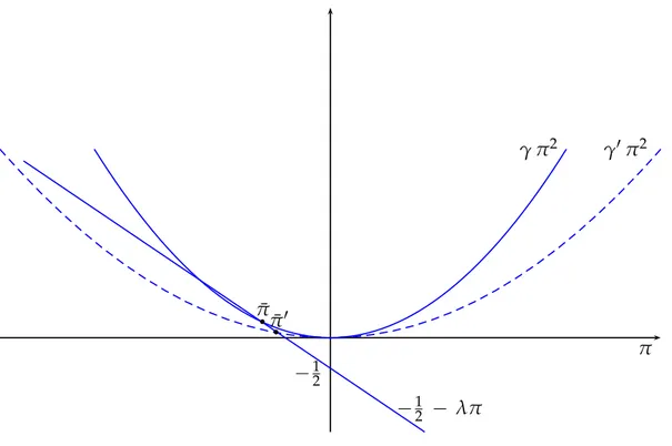
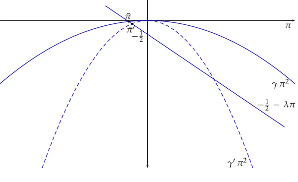
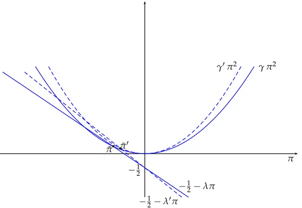
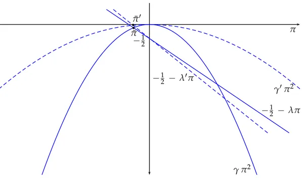
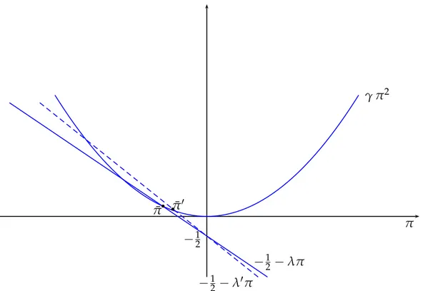
a graphical argument. In Figures A.1 and A.2 we show how the determination of ¯π+changes when eitherρ or σ2
ϵ augments. In Figure A.1 we consider the case in whichγ is positive, while in Figure
A.2 that in which it is negative.
Both Figures allow to determine what happens when an increase inρ and/or in σϵ2 brings about a reduction inγ. In both cases graphical inspection shows that for a larger degree of risk-aversion and/or a larger volatility of the demand shocks the stationary value ¯π, which is always negative,