With or without U(K): A pre-Brexit network
analysis of the EU ETS
Simone BorghesiID1,2*, Andrea FloriID3
1 FSR Climate, European University Institute, Florence, Italy, 2 Department of Political and International
Sciences, University of Siena, Siena, Italy, 3 Department of Management, Economics and Industrial Engineering, Polytechnic University of Milan, Milan, Italy
Abstract
The European Emission Trading System (EU ETS) is commonly regarded as the key pillar of the European climate policy and as the main unifying tool to create a unique carbon price all over Europe. The UK has always played a crucial role in the EU ETS, being one of the most active national registry and a crucial hub for the exchange of allowances in the market. Brexit, therefore, could deeply modify the number and directions of such exchanges as well as the centrality of the other countries in this system. To investigate these issues, the pres-ent paper exploits network analysis tools to compare the structure of the EU ETS market in its first two phases with and without the UK, investigating a few different scenarios that might emerge from a possible reallocation of the transactions that have involved UK part-ners. We find that without the UK the EU ETS network would become in general much more homogeneous, though results may change focusing on the type of accounts involved in the transactions.
Introduction
The implications of Brexit are today the object of a heated debate and have gained much atten-tion in the public opinion, both in the UK and in the rest of Europe. Among the many different consequences that Brexit could have, an important aspect concerns its impact on the EU cli-mate and energy policies and, in particular, on the European Emission Trading Scheme (henceforth EU ETS) that represents the cornerstone of the EU policy to fight climate change. The EU ETS was in fact deployed in January 2005 as the first transboundary cap-and-trade scheme and nowadays covers more than 11,000 installations from several emission-intensive sectors and across 31 States (the 28 EU Member States plus Norway, Iceland and Liechten-stein). Overall, these sectors account for about 50% of the total European CO2 emissions and 45% of all GHG emissions [1]. The EU ETS was originally divided in three phases: Phase I from 2005 to 2007, Phase II from 2008 to 2012, and Phase III from 2013 to 2020, while a new Directive [2] has been recently adopted to reform the EU ETS for Phase IV (2021-2030). The EU ETS represents the largest ETS in the world and has stimulated the adoption of similar a1111111111 a1111111111 a1111111111 a1111111111 a1111111111 OPEN ACCESS
Citation: Borghesi S, Flori A (2019) With or without
U(K): A pre-Brexit network analysis of the EU ETS. PLoS ONE 14(9): e0221587.https://doi.org/ 10.1371/journal.pone.0221587
Editor: Alessandro Spelta, Universita Cattolica del
Sacro Cuore, ITALY
Received: April 26, 2019 Accepted: August 9, 2019 Published: September 9, 2019
Copyright:© 2019 Borghesi, Flori. This is an open access article distributed under the terms of the Creative Commons Attribution License, which permits unrestricted use, distribution, and reproduction in any medium, provided the original author and source are credited.
Data Availability Statement: The data underlying
the results presented in the study are available from the European Transaction Log, URL:http://ec. europa.eu/environment/ets/transaction.do; EUROPA_JSESSIONID=2ftK1xBz5n1BQ3AYKj_ nZtcOdTm8NlFWJPCFpAN92yYt61TtXe1t! 1363888161.
Funding: SB received funding from the University
of Siena (2017-2019 Research Grant) and by the Italian Ministry of Education (PRIN). The funders had no role in study design, data collection and analysis, decision to publish, or preparation of the manuscript.
ETS in several other regions [3,4] (e.g., Alberta and Quebec in Canada, China, Japan, Kazakh-stan, South Korea, California and the Eastern part of the US).
The possible effects that Brexit could have for the EU ETS have been mainly ignored so far. Nevertheless, in our opinion, the Brexit effect on the structure and effectiveness of the EU ETS deserves greater attention being of crucial importance for the effectiveness of this instrument and for the future design of both the EU and UK climate policies. At the moment of writing the outcome of the UK-EU negotiations on the UK exit from the EU ETS appears still rather uncertain. In November 2017, UK and EU agreed that UK emitters will have to surrender car-bon units before the scheduled Brexit date. In March 2018, negotiators reached a deal on a transition period to the end of 2020, during which the UK will no longer participate in EU decision-making processes but will still be subject to the single market rules [5].
Some timely studies have started to examine how Brexit could affect the EU-UK relation-ships in terms of their climate and energy policies. For instance, changes in the UK climate policies following the vote to leave have been found to be likely to have small global economic consequences given the limited amount of UK emissions [6], but still generating a surplus of allowances in the short-term, since UK companies would want to sell their allowances that are no longer needed, and a tightening of the system in the long term [7]. In addition, studies focusing on the neighbouring states that have physical energy interconnections with the UK indicate that Brexit would have limited impact on gas and electricity prices both in UK and EU [8]. Assuming the extension of the EU ETS to non-ETS sectors in the future, numerical simu-lations find that a hard Brexit could have a negative effect on the UK’s climate policy costs and a positive one on the remaining EU member states [9]. As discussed in [10], the impact of Brexit on the remaining 27 member states would be limited if the EU accepts a weaker emis-sions cap. On the contrary, such impact is likely to be much larger for the UK in terms of increased compliance costs with its climate policy targets (estimated to range between 0.2 and 0.4 percent of its GDP), transition costs to replace the EU ETS on short notice, possible busi-ness loss as the carbon trade leaves London (that played a pivotal role as a relevant hub in the system so far), and distortions at the border due to differences between UK and EU GHG regulations.
No one has investigated so far the potential effects that Brexit could have on the structure of the EU ETS itself. The UK, in fact, plays a crucial role within the EU ETS, being one of the most active national registries with about 1,000 accounts actively involved in the exchange of allowances in the market, facilitated also by the presence of a key devoted platform for trading permits (namely, the Intercontinental Exchange—ICE). Brexit, therefore, could deeply modify the number and directions of such transactions as well as the centrality of the other registries operating in the system.
To investigate these issues, the present paper examines the structure of the EU ETS market with and without the UK, using network analysis instruments. Network theory can potentially be used to study many environmental topics [11], such as the structure of common property resources in the presence of multiple sources and users [12], how social interactions affect the adoption of eco-innovation [13], the stability of International Environmental Agreements when pollution has both global and local effects [14], how network structure influences resource exploitation [15] or global commodity trade [16] or how climate variability affects food resource availability [17]. Building upon [18], who analyze the network dynamics of the EU ETS, and [19], who use network theory to describe the structure of the EU ETS at national registry-level, in this paper we will exploit network measures to investigate the impact of Brexit on the EU ETS structure proposing a few different scenarios that might emerge from a possible reallocation of the transactions that are currently involving UK partners. Our findings indicate that, without the UK, the EU ETS would resemble a much more homogeneous network in
Competing interests: The authors have declared
which a small club of national registries would probably replace the leading role of UK, at least with respect to operations performed by pure trading accounts.
Materials and methods
Data: EU ETS transactions and account types
Data are retrieved from theEuropean Union Transaction Log—EUTL, the European
infrastruc-ture containing all available information on the transactions under the EU ETS (http://ec. europa.eu/environment/ets/transaction.do). Transactions in the EU ETS can be categorized along at least two main dimensions: i) the type of the counterparts involved in the trade, and ii) the transaction type. As to the first dimension, participants in the EU ETS can be either compliance liable entities that refer to installations responsible for greenhouse gases emissions (named, “Operator Holding Accounts”—OHAs) or voluntary accounts that operate mainly for trading purposes (named, “Person Holding Accounts”—PHAs); in addition, a bundle of players refers to governmental accounts through which allowances are managed for compli-ance purposes. As to the second dimension, transactions may be distinguished either in terms of internal vs. external exchanges (i.e., within the same national registry or across different reg-istries) or for the reason underlying the transaction (e.g., trade, issuance, allocation, surrender-ing, cancellation, correction, etc.).
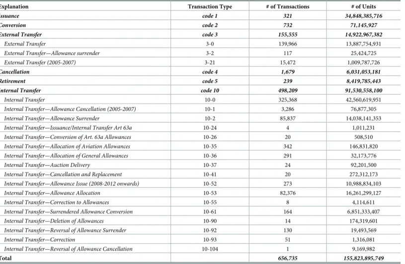
In this analysis we refer to the period from January 2005 to December 2012 in order to completely include two compliance phases, namely both Phase I and Phase II of the program. In this interval, EU ETS transactions amounted to 656, 735 operations corresponding to 155, 823, 895, 749 transferred units (seeTable 1). Total external transactions were 155, 555 (equiva-lent to about 23.68 per cent of the overall transactions) involving 14, 922, 967, 382 units being transferred. Total internal transactions were 498, 209 (75.86 per cent of all transactions) corre-sponding to 91, 530, 558, 100 units being transferred. Transactions involving OHAs and PHAs represented about 43 per cent of the transferred amount. In that period, UK transferred 26, 617, 737, 094 units and received 27, 492, 932, 700 allowances. Hence, it was responsible for more than 17 per cent of the traded units as either transferring or acquiring registry. These fig-ures confirm the relevant role of UK as a very active registry within the EU ETS.
In that period, the EU ETS was composed by the following national registries, each repre-sented as a node in the network: AT (Austria), BE (Belgium), BG (Bulgaria), CH (Switzerland), CY (Cyprus), CZ (Czech Republic), DE (Germany), DK (Denmark), EE (Estonia), ES (Spain), FI (Finland), FR (France), UK (United Kingdom), GR (Greece), HU (Hungary), IE (Ireland), IS (Iceland), IT (Italy), LI (Liechtenstein), LT (Lithuania), LU (Luxembourg), LV (Latvia), MT (Malta), NL (Netherlands), NO (Norway), PL (Poland), PT (Portugal), RO (Romania), SE (Sweden), SI (Slovenia), SK (Slovakia), UA (Ukraine). We represent with a separate node the allowances managed by the EC (European Commission), and we create the residual player
RoW to include: (i) non-EU countries having a marginal role in the system, such as AU
(Aus-tralia), JP (Japan), NZ (New Zealand), RU (Russian Federation), and (ii) allowances related to CDM (Clean Development Mechanism), the Kyoto Protocol mechanism providing allowances that may be traded in an ETS in exchange for emission reductions projects implemented in developing countries.
Network representation
Network theory techniques have been applied to study the features of a wide variety of systems (see e.g., [20] and [21]). Economic systems can be represented as a graph or networkG = (V, E), where V are the nodes representing the agents operating in the system and E stands for the
national registry, while the directed link (i, j) in E is weighted according to the number of
exchanged allowances from the transferring national registryi to the acquiring national
regis-tryj. The structure of the network is thus summarized by the adjacency matrix W, where Wij=
0 if there is not a link fromi to j, while is Wij=wijif such link exists and corresponds to the
amount of allowanceswijtransferred fromi to j.
To capture differences between the two Phases, we consider network representations for the intervals 2005-07 (Phase I) and 2008-12 (Phase II), separately. We focus on either “pure trade” transactions only (i.e., external transactions, codes 3-0 and 3-21, and internal transac-tions, code 10-0; hereinafter, theTrade specification) or the entire list of transaction types
which includes also, for instance, the issuance, allocation and surrendering of the allowances (hereinafter, theAll specification). In addition, we split data according to the two main
account types, thus focusing only on PHAs or OHAs.
To characterize the EU ETS we have applied topological measures of the nodes and network properties for the whole graph (for details on network centrality measures see [21–23], among others). Both the degree and the strength scores (and similarly their in-out variants) provide a preliminary representation of the structure of the network based on the amount of links, and possibly their weights, among connected nodes. For instance, a node with a high in-degree
Table 1. Descriptive statistics: EU ETS. First column shows the description of each transaction type. The second column indicates the codes corresponding to the
transac-tion type. The third column reports the number of transactransac-tions for each type. The fourth column shows the amount of transferred allowances. Source: authors’ own elabo-rations based on the EUTL transactions data set for the first two Phases.
Explanation Transaction Type # of Transactions # of Units
Issuance code 1 321 34,848,385,716
Conversion code 2 732 71,145,927
External Transfer code 3 155,555 14,922,967,382
External Transfer 3-0 139,966 13,887,754,931
External Transfer—Allowance surrender 3-2 117 25,424,725
External Transfer (2005-2007) 3-21 15,472 1,009,787,726
Cancellation code 4 1,679 6,031,053,181
Retirement code 5 239 8,419,785,443
Internal Transfer code 10 498,209 91,530,558,100
Internal Transfer 10-0 325,368 42,560,619,951
Internal Transfer—Allowance Cancellation (2005-2007) 10-1 3,286 76,877,305
Internal Transfer—Allowance Surrender 10-2 85,837 14,038,141,353
Internal Transfer—Issuance/Internal Transfer Art 63a 10-24 4 1,011,231
Internal Transfer—Conversion of Art. 63a Allowances 10-26 20 508,510
Internal Transfer—Allocation of Aviation Allowances 10-35 342 146,831,820
Internal Transfer—Allocation of General Allowances 10-36 291 32,173,776
Internal Transfer—Auction Delivery 10-37 24 92,201,500
Internal Transfer—Cancellation and Replacement 10-41 20 272,312,173
Internal Transfer—Allowance Issue (2008-2012 onwards) 10-52 273 10,988,834,103
Internal Transfer—Allowance Allocation 10-53 82,376 16,261,299,127
Internal Transfer—Correction to Allowances 10-55 8 4,114,611
Internal Transfer—Surrendered Allowance Conversion 10-61 164 6,851,333,407
Internal Transfer—Deletion of Allowances 10-90 14 174,319,601
Internal Transfer—Reversal of Allowance Surrender 10-92 130 19,493,569
Internal Transfer—Correction 10-93 51 1,316,081
Internal Transfer—Reversal of Allowance Cancellation 10-104 1 9,169,982
Total 656,735 155,823,895,749
refers to a registry which is able to attract transactions from many other registries of the sys-tem, while a node with high out-strength and low in- strength stands for a registry more active in transferring allowances than in acquiring them. Betweenness, closeness and eigenvector are also applied to enrich the characterization of the nodes by means of the whole configuration of the network and, in particular, of the neighborhood of each node. A node with a high value of betweenness suggests that it plays a role similar to an intermediary between many other nodes in the network, while a high value for closeness indicates that the node is likely to trade with other nodes directly. Instead, the eigenvector centrality poses importance not only in the amount of incoming links (as approximated for instance by the in-strength of the node), but it also considers how this node is connected to its neighbourhoods. As regards the network as a whole, we compute the assortativity coefficient to analyze the tendency to form connections among “similar” nodes, while centralization measures are introduced to describe the extent to which the cohesion of the graph is set around specific points. For instance, with respect to the degree distribution, the level of centralization may vary from low values corresponding to an almost complete graph to high values achieved for a star-like configuration. Finally, further topological diagnostic is provided by the diameter, the reciprocity and the transitivity. The first indicates a simple upper bound in the connectivity of the graph, the second shows the level of symmetry in links formation, while the third provides a proxy for the emergence of local clusters in the network.
In the EU ETS, for instance, not liable entities (i.e., PHAs) could opt to open accounts in certain registries according to the presence of favourable account set up requirements, fiscal advantages or the establishment of dedicated exchange platforms. Overall, these aspects can affect how national registries are connected between each other. More generally, since these conditions could have changed over time, they may have contributed to move the EU ETS from a centralized system with a few very active nodes, which were initially facilitated by infra-structure advantages, to a more uniform system.
Scenarios: With or without UK
We propose the following competing reassignment rules to study the removal of the UK from the EU ETS:
• No reassignment: we simply remove all the links in which at least one counterpart refers to
UK, but we do not reassign the corresponding amount of transferred allowances to the remaining nodes/registries;
• Proportional reassignment: we reassign links with UK as one of the counterpart to the other
national registries proportionally to the UK neighborhood. Basically, UK has a set of regis-tries from which it imports allowances (namely, its in-neighborhood) and another set to which it exports them (namely, its out-neighborhood). We allocate those links exiting from UK to registries in its neighborhood proportionally to their respective weight in the in-strength of UK, while we assign those links entering to UK to registries in its out-neighbor-hood proportionally to their respective weight in the out-strength of UK. In formula, given the in-strength of UK assIn
uk¼
PN j¼1
wj;ukand the link from UK to a certain registryx belonging
to its out-neighborhood (namely,w(uk, x)), then the latter is assigned proportionally to each
j registry in the in-neighborhood of UK as follows: ^wðj; xÞ ¼ wðj; xÞ þ wðuk; xÞ �wj;uk
sIn uk
, where the first term on the rhs refers to the true link betweenj and x and the second term indicates
the additional flow related to the proportional reassignment ofw(uk, x). Similarly, for the
in-flows into UK it will be: ^wðk; iÞ ¼ wðk; iÞ þ wðk; ukÞ �wuk;i sOut uk
• Random reassignment: the reassignment of links with UK as one of the counterpart is
per-formed randomly. This is done by generating 1000 simulated realizations, where transferred allowances referred to UK are reassigned to each combination of the remaining registries according to a weight that is drawn from a uniform distribution.
For both theProportional and Random scenarios we thus analyze a reassignment which
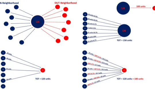
considers only transactions with UK as one of the counterpart, while those transactions involv-ing UK as both transferrinvolv-ing and acquirinvolv-ing counterparts are discarded (namely, in network jar-gon we remove the UK self-loop). The latter, in fact, refer to domestic transactions performed by UK accounts, which are therefore less likely to be alternatively operated by other accounts potentially located in other national registries.Fig 1shows a representative example of the mechanism behind the proportional reassignment, which is considered as the reference sce-nario in the study.
Results
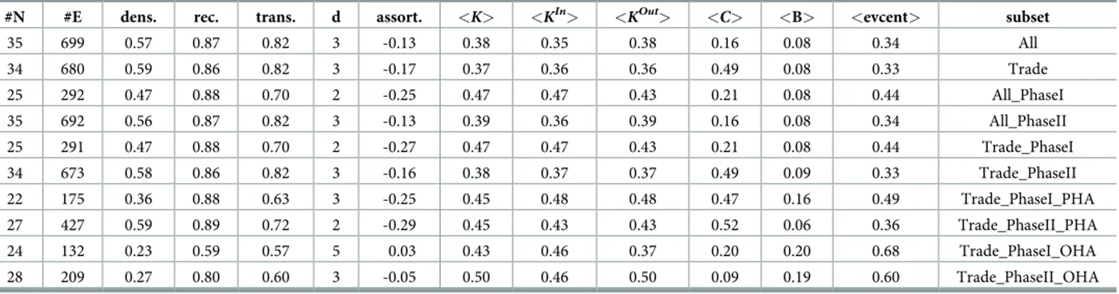
As shown inTable 2, the original system (specificationAll) is very dense, transactions between
two registries usually go in both directions, and the likelihood these nodes are part of triangles is pretty high. Hence, the EU ETS seems a very connected network and its nodes are likely to trade with many counterparts as both acquiring and transferring peers. Results are very similar if we circumscribe the analysis to the specificationTrade. Interestingly, we also notice that
despite the enlargement of the program to additional national registries (compare, e.g., #N and the diameter), Phase II coincides in general with a more connected network than the one emerging in Phase I. Finally, configurations arising from subsetting the system with only PHAs or only OHAs as both counterparts clearly highlight that the former are more connected than the latter, thus suggesting that not liable entities (i.e., PHAs) are more prone to trade
Fig 1. Example: Proportional reassignment. Plot on top-left shows the neighborhood of UK: in blue those registries
that transfer units to UK, in red those registries that acquire units from UK. Plot on the top-right isolates in red an outflow from UK to registryx (100 units), while in blue indicates the inflows of UK (a total of 150 units from registries
A-to-G). Plots on the bottom show the mechanism behind the proportional reassignment of a link exiting from UK. Bottom-left figure reports effective links from registries in the in-neighborhood of UK to registryx; bottom-right
figure explains that final links from blue nodes to the red one are the sum of the original links plus the proportional assignment of 100 units based on the weight of blue nodes in the inflows connecting them to UK.
across national registries. This may be due to the fact that PHAs mostly include brokerage firms and financial intermediaries [24], which can actually facilitate transactions across differ-ent national registries and exchange platforms. By contrast, OHAs seem more oridiffer-ented to trade with a few counterparts, thus making the related system more fragmented.
Table 2also shows that the EU ETS is a slightly disassortative network, meaning that coun-terparts usually tend to be connected with nodes dissimilar in terms of degree distribution, thus in line with other infrastructural networks (see e.g., [25–27]). This result is particularly evident in the PHAs specification, which is coherent with the activity carried out by this group: since this set of accounts mainly refers to financial intermediaries then diversification is more likely to occur and should actually be put in place by PHAs. Finally, centralization scores indicate the graph-level centrality for different centrality measures. Although the aforemen-tioned centrality measures provide different perspectives of node centrality, our findings seem to depict the EU ETS as a more centralized network during Phase I. This reasonably reflects the presence of a few very central national registries during the first years of the program, while progressively the system became less polarized. For instance, Denmark and the Nether-lands had favourable conditions to set up accounts during the early stages of the program, while other Member States such as France, Germany and the United Kingdom were among the few countries in Europe with dedicated exchange platforms for allowances. No less impor-tantly, the centrality of some national registries may have been heavily influenced by carbon carousel frauds such as that occurred in the France’s Bluenext exchange in June 2009 [28,29], which weakened the platform and contributed to its closure at the end of 2012. For instance, such episodes affected transferred volumes through France, placing this node as a very active player during the VAT fraud but then limiting its centrality once France changed its VAT rules in 2009 to respond against the fraud.
What would have been the EU ETS configuration without UK?
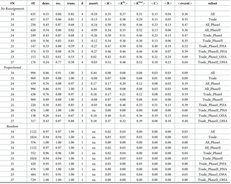
The topological investigation we will propose in this subsection offers a clear picture: the UK was involved in a huge portion of transactions which -if not performed via UK- would have been reassigned to the remaining registries producing a substantial reshuffle within the EU ETS. We can only advance some hypotheses on how these transactions might have been reas-signed. We introduce three scenarios as milestones to investigate how the EU ETS would have been without UK.
Table 2. EU ETS network diagnostic. Columns labels refer to: number of nodes (#N); number of edges (#E); density (dens); reciprocity (rec); transitivity (trans); diameter
(d); assortativity (assort). Centralization measures are indicated with symbol <x>, where x is the degree (K), the closeness (C), the betweenness (B) or the eigenvector
cen-trality (evcent). Results refer to the period 2005-2012. Source: Authors’ own elaborations.
#N #E dens. rec. trans. d assort. <K> <KIn> <KOut> <C> <B> <evcent> subset
35 699 0.57 0.87 0.82 3 -0.13 0.38 0.35 0.38 0.16 0.08 0.34 All 34 680 0.59 0.86 0.82 3 -0.17 0.37 0.36 0.36 0.49 0.08 0.33 Trade 25 292 0.47 0.88 0.70 2 -0.25 0.47 0.47 0.43 0.21 0.08 0.44 All_PhaseI 35 692 0.56 0.87 0.82 3 -0.13 0.39 0.36 0.39 0.16 0.08 0.34 All_PhaseII 25 291 0.47 0.88 0.70 2 -0.27 0.47 0.47 0.43 0.21 0.08 0.44 Trade_PhaseI 34 673 0.58 0.86 0.82 3 -0.16 0.38 0.37 0.37 0.49 0.09 0.33 Trade_PhaseII 22 175 0.36 0.88 0.63 3 -0.25 0.45 0.48 0.48 0.47 0.16 0.49 Trade_PhaseI_PHA 27 427 0.59 0.89 0.72 2 -0.29 0.45 0.43 0.43 0.52 0.06 0.36 Trade_PhaseII_PHA 24 132 0.23 0.59 0.57 5 0.03 0.43 0.46 0.37 0.20 0.20 0.68 Trade_PhaseI_OHA 28 209 0.27 0.80 0.60 3 -0.05 0.50 0.46 0.50 0.09 0.19 0.60 Trade_PhaseII_OHA https://doi.org/10.1371/journal.pone.0221587.t002
The first scenario is the one obtained by simply removing all the transactions in which UK is a counterpart; this is a limit case where we assume that exchanging allowances with UK is the main reason for that trade, so that dropping UK determines the deletion of that transaction and the impossibility to perform the same trade via a different registry. The second scenario reassigns the share of UK transactions proportionally to its neighborhood; in this scenario, we hypothesize that UK plays an intermediary role between some registries and that allowances passing through UK can be reasonably reassigned to registries in its neighborhood according to their weight in the market share of UK. The third scenario is a purely agnostic approach in which, to verify whether some properties of the network are confirmed, we randomly reassign the bundle of UK transactions to other registries without specific assumptions about the way these allowances are reallocated.Table 3summarizes the respective estimates.
Table 3. EU ETS network diagnostic: Alternative scenarios. Columns labels refer to: number of nodes (#N); number of edges (#E); density (dens); reciprocity (rec);
transi-tivity (trans); diameter (d); assortativity (assort). Centralization measures are indicated with symbol <x>, where x is the degree (K), the closeness (C), the betweenness (B)
or the eigenvector centrality (evcent). The first panel exhibits the No Reassignment scenario, the second panel shows the Proportional scenario, while the last panel reports
theRandom scenario. Results refer to the period 2005-2012. Source: Authors’ own elaborations.
#N #E dens. rec. trans. d assort. <K> <KIn> <KOut> <C> <B> <evcent> subset
No Reassignment 34 635 0.55 0.86 0.82 4 -0.10 0.35 0.37 0.31 0.15 0.04 0.36 All 33 617 0.57 0.86 0.81 3 -0.13 0.35 0.38 0.29 0.15 0.05 0.35 Trade 24 250 0.43 0.87 0.68 2 -0.24 0.50 0.50 0.46 0.23 0.13 0.47 All_PhaseI 34 628 0.54 0.86 0.82 4 -0.09 0.34 0.35 0.32 0.13 0.06 0.36 All_PhaseII 24 249 0.43 0.87 0.68 2 -0.26 0.50 0.51 0.46 0.23 0.13 0.47 Trade_PhaseI 33 610 0.56 0.85 0.81 3 -0.12 0.34 0.36 0.30 0.13 0.06 0.35 Trade_PhaseII 21 147 0.33 0.88 0.59 3 -0.27 0.47 0.50 0.50 0.49 0.19 0.52 Trade_PhaseI_PHA 26 374 0.55 0.88 0.70 2 -0.27 0.46 0.46 0.46 0.56 0.07 0.39 Trade_PhaseII_PHA 23 115 0.22 0.61 0.53 5 0.02 0.43 0.45 0.36 0.21 0.24 0.69 Trade_PhaseI_OHA 27 176 0.24 0.77 0.58 4 -0.03 0.52 0.48 0.52 0.10 0.23 0.64 Trade_PhaseII_OHA Proportional 34 996 0.86 0.91 1.00 2 0.44 0.08 0.08 0.08 0.03 0.03 0.09 All 33 969 0.89 0.88 1.00 2 -0.08 0.07 0.08 0.08 0.01 0.00 0.09 Trade 24 439 0.76 0.88 0.97 2 0.17 0.17 0.20 0.12 0.08 0.02 0.19 All_PhaseI 34 996 0.86 0.91 1.00 2 0.44 0.08 0.08 0.08 0.03 0.03 0.09 All_PhaseII 24 438 0.76 0.88 0.97 2 0.18 0.17 0.21 0.12 0.08 0.02 0.19 Trade_PhaseI 33 969 0.89 0.88 1.00 2 -0.08 0.07 0.08 0.08 0.01 0.00 0.09 Trade_PhaseII 21 220 0.50 0.85 0.85 3 -0.03 0.40 0.48 0.33 0.51 0.15 0.39 Trade_PhaseI_PHA 26 676 1.00 1.00 1.00 1 na 0.00 0.00 0.00 0.00 0.00 0.00 Trade_PhaseII_PHA 23 138 0.26 0.61 0.67 5 0.10 0.40 0.41 0.36 0.19 0.15 0.64 Trade_PhaseI_OHA 27 317 0.43 0.87 0.88 3 0.18 0.37 0.32 0.39 0.08 0.10 0.40 Trade_PhaseII_OHA Random 34 1122 0.97 0.97 1.00 1 na 0.02 0.03 0.00 0.00 0.00 0.03 All 33 1024 0.94 0.94 1.00 1 na 0.03 0.03 0.03 0.00 0.00 0.03 Trade 24 576 1.00 1.00 1.00 1 na 0.00 0.00 0.00 0.00 0.00 0.00 All_PhaseI 34 1122 0.97 0.97 1.00 1 na 0.02 0.03 0.00 0.00 0.00 0.03 All_PhaseII 24 552 0.96 0.96 1.00 1 na 0.02 0.04 0.00 0.00 0.00 0.04 Trade_PhaseI 33 1024 0.94 0.94 1.00 1 na 0.03 0.03 0.03 0.00 0.00 0.03 Trade_PhaseII 21 420 0.95 0.95 1.00 1 na 0.03 0.00 0.05 0.00 0.00 0.00 Trade_PhaseI_PHA 26 676 1.00 1.00 1.00 1 na 0.00 0.00 0.00 0.00 0.00 0.00 Trade_PhaseII_PHA 23 484 0.91 0.91 1.00 1 na 0.05 0.04 0.04 0.00 0.00 0.05 Trade_PhaseI_OHA 27 729 1.00 1.00 1.00 1 na 0.00 0.00 0.00 0.00 0.00 0.00 Trade_PhaseII_OHA https://doi.org/10.1371/journal.pone.0221587.t003
The first panel inTable 3shows the scenario obtained by simply removing UK and all the links in which UK is at least one of the counterpart of the transaction. Even in this case we notice a few differences between theAll and the Trade specifications, and we confirm the
increasing connectivity from Phase I to Phase II. More generally, the network appears slightly less dense and connected under this scenario with respect to the actual EU ETS representation reported inTable 2. Similarly, the centralization measures for both theAll and the Trade
speci-fications are usually lower than those computed for the original case. Interestingly, the parti-tion based on each Phase indicates that previous result is the combined effect of a rise in Phase I and a drop in Phase II, thus suggesting that the central role of UK seems to have been more effective during Phase II than Phase I when other national registries were very pivotal as well. Also, the subset of only PHAs shows that the removal of UK increases the centralization mea-sures in both Phases, while the OHAs specification appears much more stable with no substan-tial changes in the reported measures with and without the UK (cfr.Table 2). It is well-known, in fact, the important role played by a club of other national registries (e.g., Denmark, France, Germany, and the Netherlands) as key market places for trading allowances thanks to the pres-ence of devoted exchange platforms and favourable set-up conditions. By dropping a competi-tor as UK, their role is further enhanced and they emerge even more clearly as very pivotal nodes, especially if we focus on PHAs which are more likely to represent financial intermediar-ies very active across these stock exchanges.
The second panel inTable 3exhibits the case corresponding to theProportional scenario.
We assume that links to UK are assigned to each target node in the out-neighborhood of UK proportionally to its weight among all flows departing from the UK (i.e., its weight in the UK allowance exports flow); similarly, links exiting from UK are assigned to each source node in the in-neighborhood of UK in proportion to its weight in the in-strength of the UK (i.e., its weight in the UK allowance import flows). The network arising in this scenario is highly con-nected and dense. This is due to the fact that UK is involved in a significant share of transac-tions where it plays a role as a hub/intermediary between national registries otherwise poorly connected. By creating links between the in- and the out-neighborhood of UK, we replace the hub node represented by UK with links connecting almost every node. This occurs because UK is basically connected to each Member State of the EU ETS, which highlights the central role of UK in the program and explains why we get this very dense configuration under the
Proportional scenario. Furthermore, we still observe the same regularities already commented
about the increasing connectivity during Phase II with respect to Phase I. Note also that in this scenario the assortativity coefficient is often positive, meaning that transferring and acquiring counterparts are here much more similar than in the original case (i.e., when connected via UK). Remarkably, when we circumscribe the analysis to only PHAs, the system becomes totally connected in Phase II, thus emphasizing the role of UK as a key player in facilitating trades among market participants spread in the EU ETS. Finally, we remark that the system without UK and with proportional reassignment is very uniform as indicated by the centraliza-tion measures.
We also propose a basicRandom scenario in which UK’s links are randomly reassigned to
the remaining pairs of registries. Results in the third panel ofTable 3indicate a well-connected system in line with the discussion for theProportional scenario. Hence, if those transactions
originally performed via UK would be reassigned to the remaining nodes either proportionally to their weight in the UK’s neighborhood or even randomly, still we will get a more uniform and connected network than the actual EU ETS. A peculiar result emerges in theRandom
sce-nario if we focus on only OHAs: randomization allows to bypass some kind of country-barri-ers that force transactions for liable installations to be biased towards domestic transactions or a few other registries. Finally, as expected due to the relevant amount of transactions involving
UK, their random reassignment is able to basically generate a network configuration that is weakly structured. The removal of UK could be interpreted as a shock to the system: indeed, the agnostic reassignment of the UK-related transactions without any particular rule is likely to generate a significant perturbation which seems able to modify substantially the original configuration of the network.
Winners and losers from the removal of UK
Once a very central node like UK is dropped from the system, links will be reorganized, the centrality of the remaining nodes might result reshuffled, and the overall structure of the sys-tem may eventually change. The topological investigation discussed in the previous subsection suggests that in each of the three alternative scenarios, the removal of UK’s transactions signifi-cantly affects the configuration of the network. This subsection discusses the topological impact at the level of single nodes to detect which registries would be, eventually, more affected by such reassignment. Some registries could gain positions in the centrality rankings becoming more influential in the network, while others may reach even more peripheral positions once UK is removed. The former can be seen as the “winners” who gain from removing the UK node, while the latter are the “loosers” who, conversely, achieve even more marginal roles in the system.
To perform such analysis, the first panel ofTable 4focuses on observations related only to Phase II to provide a representation of the most recently concluded EU ETS phase (Phase III being still on-going). It also refers to the pureTrade specification because the other types of
transactions, such as the issuance, allocation and surrendering of allowances, are more coun-try-specific and affected by the relationships with governmental counterparts. Instead, the second panel ofTable 4refers to those transactions involving only PHAs to further verify vari-ations in centrality scores among those accounts (mainly financial intermediaries, banks, and brokers) for which is easier to switch across different national registries.
As shown inTable 4, we note that the UK is a very central node, while the club of the other key nodes usually encompasses: Denmark, France, Germany, the Netherlands and sometimes Italy. Together with the UK, these registries form a core of very connected nodes surrounded by a cloud of registries related to peripheral countries within the EU ETS. Among the latter it is clear that the UK plays for them a role as hub/intermediary between these nodes otherwise poorly connected, so the removal of UK without the reassignment of its links is likely to reduce the connectivity of these registries with the rest of the system. Con-versely, those already very central nodes usually appear even more central once the UK and its links are removed.
The first three blocks inTable 4refer to degree and its variants (in-degree and out-degree). These indicators provide a simple representation of the network configuration based on a binary view which assigns links regardless the transferred amount. This basic perspective is helpful for two reasons: i) it clearly indicates that Denmark, France, Germany, Italy, the Neth-erlands and the United Kingdom are key counterparts in the system being connected to almost every registry; ii) conversely, there is a cloud of less central registries mostly related to geo-graphically peripheral countries. Only a few differences appear between the first and second panel of the table; however, when we circumscribe the analysis to only PHAs (bottom panel), fewer active registries are present and some of them, e.g. Austria, Italy or Spain, appear less active compared to the configuration including the other account types (top panel).
A more effective representation of the EU ETS is offered by the second block of the topolog-ical measures (namely, strength, in-strength and out-strength). In the actual EU ETS configu-ration (case I), the UK is involved in a significant portion of transactions, although other
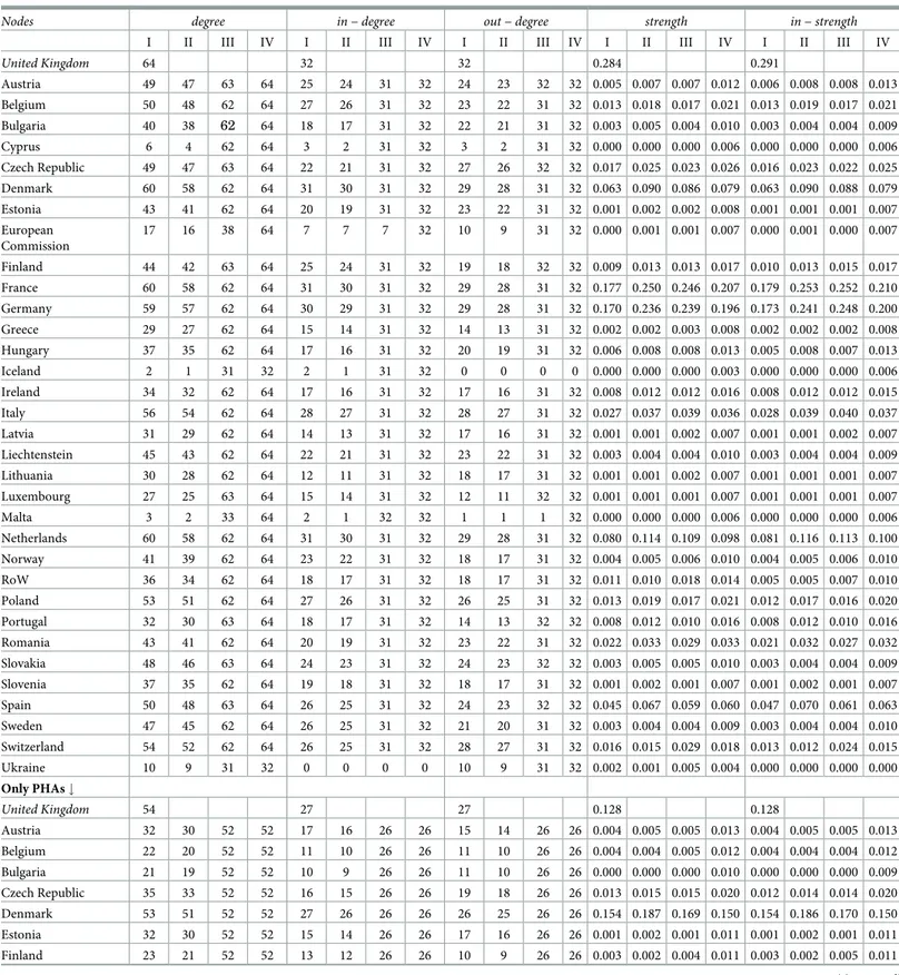
Table 4. Network centrality statistics. This table reports the following scenarios: the actualEU ETS (I), No Reassignment (II), Proportional (III), and Random (IV). Data
refer to Phase II. The first panel includes both internal and external transactions (Trade specification). The second panel refers to PHAs only. Notice that due to the
pres-ence of some registries poorly connected with the rest of the system, centrality measures for some nodes appear higher than those for the others. Source: Authors’ own elaborations.
Nodes degree in − degree out − degree strength in − strength
I II III IV I II III IV I II III IV I II III IV I II III IV
United Kingdom 64 32 32 0.284 0.291 Austria 49 47 63 64 25 24 31 32 24 23 32 32 0.005 0.007 0.007 0.012 0.006 0.008 0.008 0.013 Belgium 50 48 62 64 27 26 31 32 23 22 31 32 0.013 0.018 0.017 0.021 0.013 0.019 0.017 0.021 Bulgaria 40 38 62 64 18 17 31 32 22 21 31 32 0.003 0.005 0.004 0.010 0.003 0.004 0.004 0.009 Cyprus 6 4 62 64 3 2 31 32 3 2 31 32 0.000 0.000 0.000 0.006 0.000 0.000 0.000 0.006 Czech Republic 49 47 63 64 22 21 31 32 27 26 32 32 0.017 0.025 0.023 0.026 0.016 0.023 0.022 0.025 Denmark 60 58 62 64 31 30 31 32 29 28 31 32 0.063 0.090 0.086 0.079 0.063 0.090 0.088 0.079 Estonia 43 41 62 64 20 19 31 32 23 22 31 32 0.001 0.002 0.002 0.008 0.001 0.001 0.001 0.007 European Commission 17 16 38 64 7 7 7 32 10 9 31 32 0.000 0.001 0.001 0.007 0.000 0.001 0.000 0.007 Finland 44 42 63 64 25 24 31 32 19 18 32 32 0.009 0.013 0.013 0.017 0.010 0.013 0.015 0.017 France 60 58 62 64 31 30 31 32 29 28 31 32 0.177 0.250 0.246 0.207 0.179 0.253 0.252 0.210 Germany 59 57 62 64 30 29 31 32 29 28 31 32 0.170 0.236 0.239 0.196 0.173 0.241 0.248 0.200 Greece 29 27 62 64 15 14 31 32 14 13 31 32 0.002 0.002 0.003 0.008 0.002 0.002 0.002 0.008 Hungary 37 35 62 64 17 16 31 32 20 19 31 32 0.006 0.008 0.008 0.013 0.005 0.008 0.007 0.013 Iceland 2 1 31 32 2 1 31 32 0 0 0 0 0.000 0.000 0.000 0.003 0.000 0.000 0.000 0.006 Ireland 34 32 62 64 17 16 31 32 17 16 31 32 0.008 0.012 0.012 0.016 0.008 0.012 0.012 0.015 Italy 56 54 62 64 28 27 31 32 28 27 31 32 0.027 0.037 0.039 0.036 0.028 0.039 0.040 0.037 Latvia 31 29 62 64 14 13 31 32 17 16 31 32 0.001 0.001 0.002 0.007 0.001 0.001 0.002 0.007 Liechtenstein 45 43 62 64 22 21 31 32 23 22 31 32 0.003 0.004 0.004 0.010 0.003 0.004 0.004 0.009 Lithuania 30 28 62 64 12 11 31 32 18 17 31 32 0.001 0.001 0.002 0.007 0.001 0.001 0.001 0.007 Luxembourg 27 25 63 64 15 14 31 32 12 11 32 32 0.001 0.001 0.001 0.007 0.001 0.001 0.001 0.007 Malta 3 2 33 64 2 1 32 32 1 1 1 32 0.000 0.000 0.000 0.006 0.000 0.000 0.000 0.006 Netherlands 60 58 62 64 31 30 31 32 29 28 31 32 0.080 0.114 0.109 0.098 0.081 0.116 0.113 0.100 Norway 41 39 62 64 23 22 31 32 18 17 31 32 0.004 0.005 0.006 0.010 0.004 0.005 0.006 0.010 RoW 36 34 62 64 18 17 31 32 18 17 31 32 0.011 0.010 0.018 0.014 0.005 0.005 0.007 0.010 Poland 53 51 62 64 27 26 31 32 26 25 31 32 0.013 0.019 0.017 0.021 0.012 0.017 0.016 0.020 Portugal 32 30 63 64 18 17 31 32 14 13 32 32 0.008 0.012 0.010 0.016 0.008 0.012 0.010 0.016 Romania 43 41 62 64 20 19 31 32 23 22 31 32 0.022 0.033 0.029 0.033 0.021 0.032 0.027 0.032 Slovakia 48 46 63 64 24 23 31 32 24 23 32 32 0.003 0.005 0.005 0.010 0.003 0.004 0.004 0.009 Slovenia 37 35 62 64 19 18 31 32 18 17 31 32 0.001 0.002 0.001 0.007 0.001 0.002 0.001 0.007 Spain 50 48 63 64 26 25 31 32 24 23 32 32 0.045 0.067 0.059 0.060 0.047 0.070 0.061 0.063 Sweden 47 45 62 64 26 25 31 32 21 20 31 32 0.003 0.004 0.004 0.009 0.003 0.004 0.004 0.010 Switzerland 54 52 62 64 26 25 31 32 28 27 31 32 0.016 0.015 0.029 0.018 0.013 0.012 0.024 0.015 Ukraine 10 9 31 32 0 0 0 0 10 9 31 32 0.002 0.001 0.005 0.004 0.000 0.000 0.000 0.000 Only PHAs # United Kingdom 54 27 27 0.128 0.128 Austria 32 30 52 52 17 16 26 26 15 14 26 26 0.004 0.005 0.005 0.013 0.004 0.005 0.005 0.013 Belgium 22 20 52 52 11 10 26 26 11 10 26 26 0.004 0.004 0.005 0.012 0.004 0.004 0.004 0.012 Bulgaria 21 19 52 52 10 9 26 26 11 10 26 26 0.000 0.000 0.000 0.010 0.000 0.000 0.000 0.009 Czech Republic 35 33 52 52 16 15 26 26 19 18 26 26 0.013 0.015 0.015 0.020 0.012 0.014 0.014 0.020 Denmark 53 51 52 52 27 26 26 26 26 25 26 26 0.154 0.187 0.169 0.150 0.154 0.186 0.170 0.150 Estonia 32 30 52 52 15 14 26 26 17 16 26 26 0.001 0.002 0.001 0.011 0.001 0.002 0.001 0.011 Finland 23 21 52 52 13 12 26 26 10 9 26 26 0.003 0.002 0.004 0.011 0.003 0.002 0.005 0.011 (Continued )
Table 4. (Continued) France 49 47 52 52 24 23 26 26 25 24 26 26 0.408 0.493 0.449 0.382 0.403 0.486 0.444 0.376 Germany 52 50 52 52 26 25 26 26 26 25 26 26 0.169 0.183 0.202 0.147 0.176 0.190 0.211 0.153 Greece 23 21 52 52 11 10 26 26 12 11 26 26 0.001 0.000 0.001 0.010 0.000 0.000 0.001 0.010 Hungary 18 16 52 52 9 8 26 26 9 8 26 26 0.001 0.001 0.001 0.010 0.001 0.001 0.001 0.010 Ireland 17 15 52 52 8 7 26 26 9 8 26 26 0.002 0.001 0.003 0.010 0.002 0.001 0.004 0.010 Italy 39 37 52 52 20 19 26 26 19 18 26 26 0.018 0.014 0.025 0.020 0.017 0.016 0.022 0.021 Latvia 16 14 52 52 8 7 26 26 8 7 26 26 0.000 0.000 0.000 0.010 0.000 0.000 0.000 0.009 Liechtenstein 40 38 52 52 19 18 26 26 21 20 26 26 0.006 0.007 0.006 0.015 0.006 0.007 0.007 0.014 Lithuania 16 14 52 52 6 5 26 26 10 9 26 26 0.000 0.000 0.000 0.009 0.000 0.000 0.000 0.009 Luxembourg 17 15 52 52 8 7 26 26 9 8 26 26 0.000 0.000 0.000 0.010 0.000 0.000 0.000 0.010 Netherlands 53 51 52 52 26 25 26 26 27 26 26 26 0.047 0.042 0.062 0.041 0.048 0.042 0.064 0.041 Norway 27 25 52 52 14 13 26 26 13 12 26 26 0.002 0.001 0.003 0.010 0.002 0.001 0.002 0.010 Poland 41 39 52 52 21 20 26 26 20 19 26 26 0.009 0.011 0.010 0.018 0.009 0.011 0.010 0.018 Portugal 22 20 52 52 13 12 26 26 9 8 26 26 0.002 0.002 0.003 0.011 0.002 0.002 0.003 0.011 Romania 32 30 52 52 16 15 26 26 16 15 26 26 0.002 0.002 0.003 0.011 0.002 0.002 0.002 0.011 Slovakia 31 29 52 52 17 16 26 26 14 13 26 26 0.002 0.003 0.002 0.011 0.002 0.003 0.002 0.011 Slovenia 19 17 52 52 10 9 26 26 9 8 26 26 0.000 0.000 0.001 0.010 0.000 0.000 0.000 0.010 Spain 33 31 52 52 17 16 26 26 16 15 26 26 0.021 0.024 0.025 0.027 0.021 0.024 0.025 0.028 Sweden 37 35 52 52 18 17 26 26 19 18 26 26 0.002 0.002 0.003 0.011 0.002 0.002 0.002 0.011
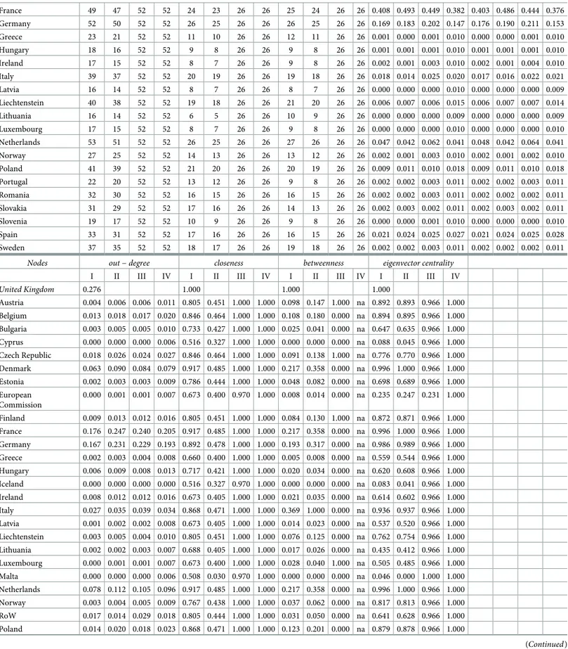
Nodes out − degree closeness betweenness eigenvector centrality
I II III IV I II III IV I II III IV I II III IV
United Kingdom 0.276 1.000 1.000 1.000 Austria 0.004 0.006 0.006 0.011 0.805 0.451 1.000 1.000 0.098 0.147 1.000 na 0.892 0.893 0.966 1.000 Belgium 0.013 0.018 0.017 0.020 0.846 0.464 1.000 1.000 0.108 0.180 0.000 na 0.894 0.895 0.966 1.000 Bulgaria 0.003 0.005 0.005 0.010 0.733 0.427 1.000 1.000 0.025 0.041 0.000 na 0.647 0.635 0.966 1.000 Cyprus 0.000 0.000 0.000 0.006 0.516 0.327 1.000 1.000 0.000 0.000 0.000 na 0.088 0.045 0.966 1.000 Czech Republic 0.018 0.026 0.024 0.027 0.846 0.464 1.000 1.000 0.091 0.138 1.000 na 0.776 0.770 0.966 1.000 Denmark 0.063 0.090 0.084 0.079 0.917 0.485 1.000 1.000 0.217 0.358 0.000 na 0.996 1.000 0.966 1.000 Estonia 0.002 0.003 0.003 0.009 0.786 0.444 1.000 1.000 0.048 0.082 0.000 na 0.698 0.689 0.966 1.000 European Commission 0.000 0.001 0.001 0.007 0.673 0.400 0.970 1.000 0.008 0.014 0.000 na 0.235 0.247 0.231 1.000 Finland 0.009 0.013 0.012 0.016 0.805 0.451 1.000 1.000 0.084 0.130 1.000 na 0.872 0.871 0.966 1.000 France 0.176 0.247 0.240 0.205 0.917 0.485 1.000 1.000 0.217 0.358 0.000 na 0.996 1.000 0.966 1.000 Germany 0.167 0.231 0.229 0.193 0.892 0.478 1.000 1.000 0.193 0.317 0.000 na 0.986 0.989 0.966 1.000 Greece 0.002 0.003 0.004 0.008 0.660 0.400 1.000 1.000 0.005 0.008 0.000 na 0.559 0.544 0.966 1.000 Hungary 0.006 0.009 0.008 0.013 0.717 0.421 1.000 1.000 0.020 0.034 0.000 na 0.620 0.608 0.966 1.000 Iceland 0.000 0.000 0.000 0.000 0.516 0.327 0.970 1.000 0.000 0.000 0.000 na 0.083 0.041 0.966 1.000 Ireland 0.008 0.012 0.012 0.016 0.673 0.405 1.000 1.000 0.021 0.035 0.000 na 0.614 0.602 0.966 1.000 Italy 0.027 0.035 0.039 0.034 0.868 0.471 1.000 1.000 0.369 1.000 0.000 na 0.936 0.937 0.966 1.000 Latvia 0.001 0.002 0.002 0.008 0.673 0.405 1.000 1.000 0.014 0.023 0.000 na 0.537 0.520 0.966 1.000 Liechtenstein 0.003 0.005 0.004 0.010 0.805 0.451 1.000 1.000 0.076 0.125 0.000 na 0.762 0.754 0.966 1.000 Lithuania 0.002 0.002 0.003 0.007 0.688 0.405 1.000 1.000 0.017 0.026 0.000 na 0.435 0.412 0.966 1.000 Luxembourg 0.000 0.001 0.001 0.007 0.673 0.400 1.000 1.000 0.028 0.040 1.000 na 0.505 0.485 0.966 1.000 Malta 0.000 0.000 0.000 0.006 0.508 0.030 0.970 1.000 0.000 0.000 0.000 na 0.046 0.000 1.000 1.000 Netherlands 0.078 0.112 0.105 0.096 0.917 0.485 1.000 1.000 0.217 0.358 0.000 na 0.996 1.000 0.966 1.000 Norway 0.003 0.004 0.005 0.009 0.767 0.438 1.000 1.000 0.037 0.062 0.000 na 0.817 0.813 0.966 1.000 RoW 0.017 0.014 0.029 0.018 0.805 0.444 1.000 1.000 0.031 0.050 0.000 na 0.641 0.628 0.966 1.000 Poland 0.014 0.020 0.018 0.023 0.868 0.471 1.000 1.000 0.123 0.201 0.000 na 0.879 0.878 0.966 1.000 (Continued )
registries are also very active either in terms of transferring or acquiring operations. France and Germany, for instance, would be the most central nodes in the network once the UK is removed, while those registries in the periphery would continue to play a marginal role. In the PHAs specification, the UK is not the most central node and the reassignment of its links clearly identifies France as the key node in the network under all the alternative scenarios. More specifically, theRandom scenario (case IV) penalizes very central nodes (e.g., Denmark,
France, and Germany) with respect to the actual EU ETS configuration, while theProportional
scenario (case III) coincides with a gain in centrality for these registries. The latter are relevant transferring and acquiring counterparts for the UK and would proportionally receive the lion’s share of its transactions once the UK is removed.
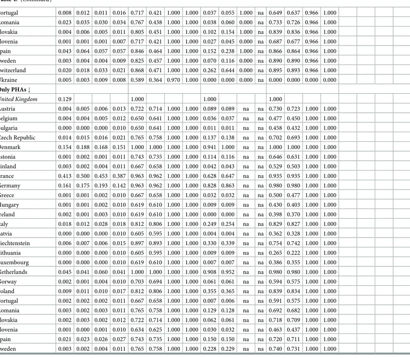
Table 4. (Continued) Portugal 0.008 0.012 0.011 0.016 0.717 0.421 1.000 1.000 0.037 0.055 1.000 na 0.649 0.637 0.966 1.000 Romania 0.023 0.035 0.030 0.034 0.767 0.438 1.000 1.000 0.038 0.060 0.000 na 0.733 0.726 0.966 1.000 Slovakia 0.004 0.006 0.005 0.011 0.805 0.451 1.000 1.000 0.102 0.154 1.000 na 0.839 0.836 0.966 1.000 Slovenia 0.001 0.001 0.001 0.007 0.717 0.421 1.000 1.000 0.027 0.045 0.000 na 0.687 0.677 0.966 1.000 Spain 0.043 0.064 0.057 0.057 0.846 0.464 1.000 1.000 0.152 0.238 1.000 na 0.866 0.864 0.966 1.000 Sweden 0.003 0.004 0.004 0.009 0.825 0.457 1.000 1.000 0.070 0.116 0.000 na 0.890 0.890 0.966 1.000 Switzerland 0.020 0.018 0.033 0.021 0.868 0.471 1.000 1.000 0.262 0.644 0.000 na 0.895 0.893 0.966 1.000 Ukraine 0.005 0.003 0.009 0.008 0.589 0.364 0.970 1.000 0.000 0.000 0.000 na 0.000 0.000 0.000 0.000 Only PHAs # United Kingdom 0.129 1.000 1.000 1.000 Austria 0.004 0.005 0.006 0.013 0.722 0.714 1.000 1.000 0.089 0.089 na na 0.730 0.723 1.000 1.000 Belgium 0.004 0.004 0.005 0.012 0.650 0.641 1.000 1.000 0.036 0.037 na na 0.477 0.450 1.000 1.000 Bulgaria 0.000 0.000 0.000 0.010 0.650 0.641 1.000 1.000 0.011 0.011 na na 0.458 0.432 1.000 1.000 Czech Republic 0.014 0.015 0.016 0.021 0.765 0.758 1.000 1.000 0.137 0.138 na na 0.702 0.693 1.000 1.000 Denmark 0.154 0.188 0.168 0.151 1.000 1.000 1.000 1.000 0.941 1.000 na na 1.000 1.000 1.000 1.000 Estonia 0.001 0.002 0.001 0.011 0.743 0.735 1.000 1.000 0.114 0.116 na na 0.646 0.631 1.000 1.000 Finland 0.003 0.002 0.004 0.011 0.667 0.658 1.000 1.000 0.042 0.043 na na 0.529 0.503 1.000 1.000 France 0.413 0.500 0.453 0.387 0.963 0.962 1.000 1.000 0.628 0.647 na na 0.935 0.935 1.000 1.000 Germany 0.161 0.175 0.193 0.142 0.963 0.962 1.000 1.000 0.828 0.863 na na 0.980 0.980 1.000 1.000 Greece 0.001 0.001 0.002 0.010 0.667 0.658 1.000 1.000 0.032 0.032 na na 0.500 0.477 1.000 1.000 Hungary 0.001 0.001 0.002 0.010 0.619 0.610 1.000 1.000 0.009 0.009 na na 0.430 0.403 1.000 1.000 Ireland 0.002 0.001 0.003 0.010 0.619 0.610 1.000 1.000 0.000 0.000 na na 0.398 0.370 1.000 1.000 Italy 0.018 0.012 0.028 0.018 0.812 0.806 1.000 1.000 0.249 0.254 na na 0.829 0.827 1.000 1.000 Latvia 0.000 0.000 0.000 0.010 0.605 0.595 1.000 1.000 0.004 0.004 na na 0.362 0.328 1.000 1.000 Liechtenstein 0.006 0.007 0.006 0.015 0.897 0.893 1.000 1.000 0.330 0.339 na na 0.754 0.742 1.000 1.000 Lithuania 0.000 0.000 0.000 0.010 0.605 0.595 1.000 1.000 0.009 0.009 na na 0.265 0.222 1.000 1.000 Luxembourg 0.000 0.000 0.000 0.010 0.619 0.610 1.000 1.000 0.007 0.007 na na 0.386 0.355 1.000 1.000 Netherlands 0.045 0.041 0.060 0.041 1.000 1.000 1.000 1.000 0.908 0.952 na na 0.980 0.980 1.000 1.000 Norway 0.002 0.001 0.004 0.010 0.703 0.694 1.000 1.000 0.061 0.061 na na 0.594 0.575 1.000 1.000 Poland 0.009 0.011 0.010 0.017 0.812 0.806 1.000 1.000 0.355 0.365 na na 0.839 0.834 1.000 1.000 Portugal 0.002 0.002 0.002 0.011 0.667 0.658 1.000 1.000 0.007 0.006 na na 0.591 0.575 1.000 1.000 Romania 0.003 0.002 0.003 0.011 0.765 0.758 1.000 1.000 0.129 0.128 na na 0.692 0.682 1.000 1.000 Slovakia 0.002 0.003 0.002 0.012 0.722 0.714 1.000 1.000 0.062 0.061 na na 0.718 0.709 1.000 1.000 Slovenia 0.001 0.000 0.001 0.010 0.634 0.625 1.000 1.000 0.030 0.032 na na 0.463 0.437 1.000 1.000 Spain 0.021 0.023 0.026 0.027 0.743 0.735 1.000 1.000 0.150 0.150 na na 0.720 0.711 1.000 1.000 Sweden 0.003 0.002 0.004 0.011 0.765 0.758 1.000 1.000 0.228 0.229 na na 0.740 0.731 1.000 1.000 https://doi.org/10.1371/journal.pone.0221587.t004
Subsequent blocks ofTable 4present centrality indicators more related to the overall net-work and the way each node is connected to the rest of the system. These measures may not be necessarily positively correlated between each other [30]. An example about the relationships between these centrality measures under each alternative scenario is presented inS1 Fig. Closeness can be interpreted as a measure of how long it will take to spread information from a certain node to all the other nodes sequentially. In the first panel, the UK is among the most central nodes in terms of closeness. Some geographically peripheral registries (e.g., Cyprus, Malta, Iceland, and Ukraine) are more distant from the rest of the system, while in general only a few links are needed to connect each node to the others. Almost all registries are con-nected to the others on average by a couple of steps. Instead, as expected, values for closeness measures would fall if we remove the UK and we do not reassign the corresponding links (case II), while they would increase if we reassign them proportionally to its neighborhood (case III). Overall, this finding confirms that the UK facilitates connections among different parts of the EU ETS. Configurations for only PHAs are dense and highly connected with the UK play-ing a prominent role, although other registries are very central and remain so even if we drop the UK without reassigning its links. Hence, within the PHAs, the system appears well con-nected and removing the UK does not significantly reduce the distance between registries.
Betweenness indicates how frequently a node lies along the geodesic pathways connecting other nodes, thus representing an asymmetric measure of centrality. The UK is the most cen-tral node in this framework, thus emphasizing its role as hub/intermediary between different parts of the network. Denmark, France, Germany, Italy, the Netherlands and Switzerland form a club of central nodes and they benefit more than others from the drop of the UK. Their centrality scores, although higher than those of most other registries, are far from the UK’s value, thus supporting the interpretation that the latter is the only key node in that framework. Instead, if we focus on PHAs only, other nodes appear very central: Denmark, Germany, and the Netherlands are, in fact, almost as central as the UK, while most of the remaining nodes are peripheral.
Finally, we consider the eigenvector centrality. Again the club composed by Denmark, France, Germany, Italy, the Netherlands and UK reach very high central scores, while in the bottom part of the ranking there are those geographically peripheral countries already seen in the previous centrality measures. The eigenvector is an appealing indicator of centrality since it does not only consider the amount of flows impacting to a certain node (as already mea-sured, e.g., by the strength), but it also consider the structure of the network and, in particular, of the nearest nodes from and to which the node operates transactions. Hence, it is worth remarking that central nodes in terms of eigenvector are not necessarily related to registries with high inflows (see, e.g., the high values of the eigenvector centrality for Austria, Finland or Slovakia). In general, removing the UK without reassigning its link causes peripheral nodes to become slightly more marginal, while for more central nodes the effect is spurious. In the PHAs specification, the ranking is instead more clear, especially in the upper tail of the distri-bution. Denmark, France, Germany, and the Netherlands are the most central nodes together with the UK, and the removal of the latter node (without reassignment) basically decreases only the centrality scores of the remaining less central nodes.Proportional and Random
sce-narios are almost fully connected networks, thus the indicator reaches its maximum value. The second panel ofTable 4is likely to represent the most plausible scenario arising from the removal of the UK, since it deals with non-liable entities (namely, PHAs) that can easily switch into a different national registry for trading purposes. This subsection suggests that removing the UK may induce non-liable entities to move from the UK to already very central registries, which are also characterized by the presence of devoted exchanges for trading allowances.
Discussion
The UK has always played a pivotal role in the EU ETS: it is the second-largest GHG emitter in the EU and has long been one of the most ambitious countries in terms of climate policies and targets within the EU. The UK ETS was the first, multi-sector emission trading program and its experience somehow inspired the EU ETS. For all these reasons, if the UK decides to leave the EU ETS after Brexit, this will obviously have significant impacts on the EU ETS (though these might as well be smaller than those on the UK itself).
This study exploits network analysis tools to assess the role played by the UK in the EU ETS and to compare the actual structure of the system (including the UK) with the one that would have emerged without the UK under different scenarios. In particular, in the (basic but proba-bly most realistic) proportionality scenario we evaluate how the structure would change if the large import and export flows involving the UK registry were reassigned to its partners in pro-portion to their weight in the UK relationships.
When the UK is removed from the system the structure of the network turns out to change deeply. Indeed, in some of the configurations taken into account (e.g. theTrade specification
that encompasses both internal and external transactions) the UK was basically an outlier. In these cases the departure of the UK would transform the network from an almost star-like sys-tem (the UK being at the centre of the star and its partners surrounding it) to a core-periphery structure with a club of core countries (Denmark, France, Germany, Netherlands, partly Italy) becoming more central in the network while the others remain at the periphery of the system. As one would expect, therefore, the structure of the EU ETS is not persistent to a large shock such as the UK exit from the system. However, this does not seem to apply to the network composed of PHAs only. In fact, the PHAs network is already very connected and more homo-geneous and it is likely to remain so, with or without the UK. This reflects the very nature of PHAs which, being mainly financial intermediaries, are more likely to trade across national borders, thus establishing links across all nodes within the PHAs network.
Supporting information
S1 Fig. In- vs. strength distributions. Plot shows the distributions of in-strength vs.
out-strength in Phase II. Panela) is the All case; b) is the Trade case; c) is the Trade case for only
OHAs;d) is the Trade case for only PHAs. Colors refer to: the actual EU ETS (designated with
purple); theNo reassignment case (in red); the Proportional case (in green); and the Random
case (in blue). Only very central nodes are highlighted in color, while the orthogonal dotted lines refer to UK under the actual EU ETS network and are introduced as a reference point. Source: Authors’ own elaborations.
(PDF)
Acknowledgments
The authors would like to thank seminar participants at the Workshop “Post-Brexit EU-UK Cooperation in Climate and Energy Policy” (10 April 2018, European University Institute, Florence) and at the 6th World Congress of Environmental and Resource Economists (25–29 June 2018, Gothenburg) for helpful comments and suggestions on a preliminary version of this paper. The usual disclaimer applies.
Author Contributions
Data curation: Andrea Flori. Formal analysis: Andrea Flori. Methodology: Simone Borghesi.
Writing – original draft: Simone Borghesi, Andrea Flori. Writing – review & editing: Simone Borghesi, Andrea Flori.
References
1. European Commission. EU ETS Handbook European Commission, DG Climate Action (CLIMA). 2015.
2. European Parliament and Council of the European Union. Directive (EU) 2018/410 of the European Parliament and of the Council of 14 March 2018 amending Directive 2003/87/EC to enhance cost-effec-tive emission reductions and low-carbon investments, and Decision (EU) 2015/1814 Official Journal of the European Union, 19/3/2018.
3. Ellerman AD, Convery FJ, De Perthuis C. Pricing carbon: the European Union emissions trading scheme. Cambridge University Press. 2010.
4. World Bank, Ecofys. State and Trends of Carbon Pricing 2018. World Bank Publications. Washington, DC, 2018.
5. Carbon Pulse. EU, UK reach deal on transition period to the end of 2020.https://carbon-pulse.com/ 49217/. Published on March 19, 2018.
6. Hepburn C, Teytelboym A. Climate change policy after Brexit. Oxford Review of Economic Policy. 2017; 33(suppl_1), S144–S154.https://doi.org/10.1093/oxrep/grx004
7. European Union. The Impact of Brexit for the EU energy system. Directorate-General for Internal Poli-cies Policy Department A: Economic and Scientific Policy, Bruxelles. 2017.
8. Pollitt MG, Chyong K. A Brexit and its Implications for British and EU Energy and Climate Policy. Centre on Regulation in Europe (CERRE): Brussels, Belgium. 2017.
9. Babonneau FLF, Haurie A, Vielle M. Welfare implications of EU effort sharing decision and possible impact of a hard Brexit. Energy Economics. 2018; 74: 470–489.https://doi.org/10.1016/j.eneco.2018. 06.024
10. Tol RSJ. Policy Brief—Leaving an Emissions Trading Scheme: Implications for the United Kingdom and the European Union. Review of Environmental Economics and Policy. 2017; 12(1), 183–189.https:// doi.org/10.1093/reep/rex025
11. Currarini S, Marchiori C, Tavoni A. Network economics and the environment: insights and perspectives. Environmental and Resource Economics. 2016; 65(1), 159–189. https://doi.org/10.1007/s10640-015-9953-6
12. İlkılıc¸ R. Networks of common property resources. Economic Theory. 2011; 47(1), 105–134.https://doi. org/10.1007/s00199-010-0520-7
13. Conley T, Udry C. Social learning through networks: The adoption of new agricultural technologies in Ghana. American Journal of Agricultural Economics. 2001; 83(3), 668–673.https://doi.org/10.1111/ 0002-9092.00188
14. Gu¨nther M, Hellmann T. International environmental agreements for local and global pollution. Journal of Environmental Economics and Management. 2017; 81, 38–58.https://doi.org/10.1016/j.jeem.2016. 09.001
15. Kyriakopoulou E, Xepapadeas A. Natural Resource Management: A Network Perspective. World Con-gress of Environmental and Resource Economists, Gothenburg, June 25-29. 2018.
16. Kharrazi A, Rovenskya E, Fath BD. Network structure impacts global commodity trade growth and resil-ience. PloS one. 2017; 12.2: e0171184.https://doi.org/10.1371/journal.pone.0171184PMID:28207790 17. Dolfing AG, Leuven JRFW, Dermody BJ. The effects of network topology, climate variability and shocks on the evolution and resilience of a food trade network. PloS one. 2019; 14.3: e0213378.https://doi.org/ 10.1371/journal.pone.0213378PMID:30913228
18. Karpf A, Mandel A, Battiston S. Price and network dynamics in the European carbon market. Journal of Economic Behavior & Organization. 2018; 153: 103–122.https://doi.org/10.1016/j.jebo.2018.06.019 19. Borghesi S, Flori A. EU ETS Facets in the Net: Structure and Evolution of the EU ETS Network. Energy
Economics. 2018; 75, 602–635.https://doi.org/10.1016/j.eneco.2018.08.026
20. Newman MEJ. The structure and function of complex networks mixing in networks. SIAM review. 2003; 45(2), 167–256.https://doi.org/10.1137/S003614450342480
21. Jackson MO. Social and economic networks. Princeton University Press. 2010.
22. Newman MEJ. Networks. Oxford university press. 2018.
23. Caldarelli G. Scale-free networks: complex webs in nature and technology. Oxford University Press. 2007.
24. Betz RA, Schmidt TS. Transfer patterns in Phase I of the EU Emissions Trading System: a first reality check based on cluster analysis. Climate Policy. 2016; 16(4), 474–495.https://doi.org/10.1080/ 14693062.2015.1028319
25. Bagler G. Analysis of the airport network of India as a complex weighted network. Physica A: Statistical Mechanics and its Applications. 2008; 387(12), 2972–2980.https://doi.org/10.1016/j.physa.2008.01. 077
26. Chopra SS, Dillon T, Bilec MM, Khanna V. A network-based framework for assessing infrastructure resilience: a case study of the London metro system. Journal of The Royal Society Interface. 2016; 13 (118), 20160113.https://doi.org/10.1098/rsif.2016.0113
27. Cotilla-Sanchez E, Hines PDH, Barrows C, Blumsack S. Comparing the topological and electrical struc-ture of the North American electric power infrastrucstruc-ture. IEEE Systems Journal. 2012; 6(4), 616–626.
https://doi.org/10.1109/JSYST.2012.2183033
28. Europol. Further investigations into VAT fraud linked to the carbon emissions trading system. Europol. 2010.
29. Frunza MC, Guegan D, Lassoudiere A. Missing trader fraud on the emissions market Journal of finan-cial crime. 2011; 18(2), 183–194.https://doi.org/10.1108/13590791111127750
30. Valente TW, Coronges K, Lakon C, Costenbader E. How correlated are network centrality measures?. Connections (Toronto, Ont.). 2008; 28(1), 16.