Alteration and Contamination of Archaeological Ceramics: the Perturbation Problem

http://www.sciencedirect.com/science/article/pii/S0305440398903909

DOI: 10.1006/jasc.1998.0390 (http://dx.doi.org/10.1006/jasc.1998.0390)

ALTERATION AND CONTAMINATION OF ARCHAEOLOGICAL CERAMICS: THE PERTURBATION PROBLEM.

J. Buxeda i Garrigós

ALTERATION AND CONTAMINATION OF ARCHAEOLOGICAL CERAMICS: THE PERTURBATION PROBLEM.

J. Buxeda i Garrigós (Laboratory of Archaeometry, NCSR "Demokritos", 15310 Aghia Paraskevi, Attiki, Greece).

Abstract.

Alteration and contamination processes modify the chemical composition of ceramic artefacts. This is not restricted solely to the affected elements, but also affects general concentrations. This is due to the compositional nature of chemical data, enclosed by the restriction of unit sum. Since it is impossible to know prior to data treatment whether the original compositions have been changed by such processes, the methodological approach used in provenance studies must be robust enough to handle materials that might have been altered or contaminated. The ability of the logratio transformation proposed by Aitchinson to handle compositional data is studied and compared with that of present data treatments. The logratio transformation appears to offer the most robust approach.

Key words.

Alteration, contamination, perturbation, logratio transformation, variation matrix, statistical treatment, provenance, ceramics.

Introduction.

The two main principles of provenance studies through chemical characterisation were formally established in the 70s: On the one hand, the equation which models all sources of variation (Bieber et al., 1976):

varT=varN+varS+varA, (1)

where varT is the total variance in the determination of concentration of one particular

element for one individual, varN the natural variance, varS the sampling variance, and

varA the analytical variance (vid. Beier & Mommsen, 1994); and on the other hand,

the provenance postulate: "...namely that there exist differences in chemical composition between different natural sources that exceed, in some recognisable way, the differences observed within a given source." (Weigand et al., 1977, 24). Both principles are related and both point to compositional variability as being the basic principle in chemical characterisation.

As used in (1), the term 'natural' simplifies a more complex reality. In addition to the differences that exist between two raw materials of different origin, there are three distinct stages in pottery fabrication that must be taken into consideration as each can introduce variability through the particular technological processes involved. In the first stage, there is the selection of one or more raw materials, which contain the information of provenance (which is not necessarily the same as that of the the pottery, if trade in raw materials have occurred). In the second stage, there exists the variability introduced by the potter during the preparation of one or more pastes, depending on the particular use the pottery is to be put to (Steponaitis, 1984; Cuomo di Caprio, 1985; Arnold, 1992). Finally, the paste can be diversified during firing,

resulting in different transformations which affect mineralogy (Maggetti, 1981), chemical composition (Widemann et al., 1975; Kilikoglou et al., 1988), as well as physical properties including microstructure and colour (Picon, 1973; Tite & Maniatis, 1975; Dufournier, 1982; Béarat et al., 1989). As a result of these changes a paste may then result in the production of one or more fabrics (adapted from Whitbread, 1989, 127). Therefore, in case studies the relation between the paste and the derived fabrics should be satisfactorily explained by a model of transformation during firing, which can then be verified by experimental work (Buxeda et al., 1995). In addition to these three stages, there exists another source of variability, which is the subject of this paper. This final source of variability refers to unintentional alteration and contamination processes that take place during the phases of manufacture, use, burial, excavation, conservation and analysis.

It was at the end of the 60s and the beginning of the 70s, when the processes of alteration and contamination of pottery were first taken into consideration (Freeth, 1967; Millet, 1967; Matson, 1971; Sayre et al., 1971; Duma, 1972). In subsequent years, there has been a not unexpected increase in research in this field, and considerable advances have been made (Béarat, 1990; Picon, 1991). Surprisingly, the effects of alteration and contamination processes on chemical composition have not received the same level of attention. Studies almost exclusively focus on the variations observed in the elements directly affected by these processes. As far as we know, only Picon (1986) has proposed a general correction of the elemental concentrations determined as well as recently pointing out the implications of the ‘residual distances’ that exist when we compare one individual with a previously established reference group (Picon, 1992; Morel & Picon, 1995).

The main purpose of this paper is the theoretical study of the implications that alteration and contamination processes have on elemental concentrations, and their effect on the treatment of the chemical data.

The perturbation problem.

Alteration and contamination processes modify the original composition according to the properties of compositional data. The operation introduced by Aitchinson (1986, 42-43 and 123-125)

x1=u1°x0=C(x0 1u1 1,...,x0 Du1 D) (2)

is defined as perturbation. During that operation, the D-parts compositional vector x0,

which we can identify with the original compositional vector of a ceramic artefact, is operated by the D-parts perturbing vector u1 of positive elements. The result is the

perturbed compositional vector x1. C represents the constraining operator which

transforms each D-parts vector in one vector with unit sum. A generalisation of (2), for the processes that involve a sequence of compositions generated by independent successive perturbations, is possible according to the rules of the ° operator (Aitchinson, 1992):

xn=u°x (x=x0;u=(un°...°u1) (n=1,2,...)). (3)

Thus, taking expression (3) as a starting point, we are able to develop a theory of alteration processes which can deal with more than one perturbation operation.

The values of the components of the perturbing vector will be in the range 0<uj<1 when the perturbation implies a drop in the concentration of the xj component

of the compositional vector, or uj>1 if it implies an increment. Finally, the value will

be uj=1 if it does not imply any change. Thus, 1 is the neutral element for the

perturbation. Then, the operation of perturbation of one compositional vector by one perturbing vector with all its components uj=1 (j=1,...,D), is the identity perturbation.

Now, taking (2) and (3) together, we can develop these expressions to

x_n u x _{D D} j j j D D D j j j D x u x u x u x u x u x u = ° = = = =

∑

∑

and, developing the denominator as

x u_{j j} x u x x u_{D D} x_D k j D = + − + + − = =

∑

we arrive to the expression

xn D D D D x u k x u k x u k x u k =100 1 1 = 100 1 1 100 ( ,..., ) ( ( ),..., ( )). (5)

Note that in these developments the constant 100 has been introduced in order to express the data in percentage values.

According to (5), we can verify that in fact the perturbation operation in compositional data establishes two types of perturbation. The first, which we shall call direct, comes from the fact that one component xj is multiplied by one component uj,

as is established in (2). The second, which we shall call indirect, comes from the fact that one component xj is divided by the value k defined in (4) and is a perturbation

imposed by the constraining operator. Thus, the possible sources of variation in the D components of x0 are actually the direct and indirect perturbations present in all the

perturbation operations.

The value k, as expressed in (4), is the result of the sum of the D components of the original compositional vector x0 plus those terms ((xjuj)-xj) (j=1,...,D) which

are not cancelled when being operated by the neutral element (i.e. uj≠1). Therefore,

the fact that k deviates from 100 depends only on those components of the perturbing vector other than the neutral element. Moreover, it is clear that 100 is the neutral element of the indirect operation because it cancels the indirect operation. Nevertheless, it is possible for k to assume the value of 100,if there are two or more terms ((xjuj)-xj) with uj≠1 producing equal perturbations but in opposite directions. At

the same time, a discrepancy appears between the expected value from the direct perturbation operation and the observed value which arises from the final indirect operation. In this sense, the value determined by the chemical analysis is an overestimation of that value resulting from the direct perturbation if k<100 and, on the contrary, it is an underestimation if k>100.

It is clear from the above that the validity of a methodology able to deal with perturbed data depends on its ability to avoid the effects of the indirect operations, because the latter become a source of spurious error propagation with no connection to the natural processes, but rather to the constraining operator of the compositional data. At the same time, having proved its ability to cancel the indirect operations, it would be desirable for such a methodology to facilitate the identification of the effects of the direct operations, in order that they might be recognised and taken into consideration.

Traditional data treatments.

Traditional data treatments use the data in one of two ways. The raw data can be either used in their original values or by taking their logarithms; or some scholars normalise the subcompositions in such a way that the sum of the determined components is 100. The main reason for doing this is to achieve a better intercomparability of the elemental concentrations of the same component in two different compositional vectors. This is a common way of working on subcompositions that include the most of major and minor elements. However, it is not used at all by those who determine almost exclusively trace elements.

The compositional vectors in chemical characterisation have no D random dimensions, but rather the D dimensions are the number of elements in the Periodical System that occur naturally. However, in practice the analytical determinations are never performed for all the D components, but for a subcomposition S (S<D) that is imposed by either the technical possibilities, the theoretical assumptions, or both factors together. Therefore, (5) can be written as

xSubc n S S x u k x u k =(100( 1 1),...,100( )). (6)

It is important to consider that, in (6), k has the same meaning given by (4). Thus, the elemental concentrations of the determined subcomposition are affected by the direct perturbations which depend on the components uj (j=1,...,S), but they are also affected

by the indirect perturbations that are dependent on all the components uj (j=1,...,D).

Expression (6) actually forms the basis for those data treatments conducted on the raw data.

However, in the case where the subcomposition is normalised we start from another basis: xSubcNor n Subc n S S x x u k x u k =100C =100C 100 1 1 ,...,100 ( ) ( ( ) ( )).

Due to the constraining operator, imposed during normalisation, a second indirect operation is performed by a new value which is similar to the value k defined in (4). This new value is formed only from the values of the S components of the determined subcomposition: k x u k x u k k x u x u Subc S S S S =100 1 1 + +100 =100 + + 1 1 ( ) ... ( ) (( ) ... ( )).

Thus, the resulting expression can be written as

xSubcNor n Subc S S Subc S S x u k k x u k k x u c x u c =100 = 100 100 100 100 1 1 1 1 ( ( ) ,..., ( ) ) ( ( ),..., ( )) , (7) where c corresponds to c=(x1u1)+...+(xSuS). (8)

Expressions (7) and (8) allow us to confirm the intuitive idea that the normalisation of the subcompositions produces new values that are independent of the undetermined components and, more importantly, that are independent of those undetermined components of the perturbing vector. In spite of this corrective effect, other problems exist in using the normalised subcompositions, because the normalisation finally multiplies each component of the determined subcomposition by a scale factor

a c

=100, (9)

where c has the meaning defined by (8).

These developments clearly show that working with the elemental concentration of the determined subcompositions, either with the raw data, or with the normalised subcompositions, implies several serious problems, mainly because the determined concentrations depend, through the indirect operation, on the value k defined by (4) for the raw data, or on the scale factor a defined by (9) for the normalised subcompositions.

On top of these problems, two other objections need to be raised. First, intra-vector ratios are maintained for those components directly operated by the same value in the perturbing vector, but not necessarily for the inter-vector ratios. Expressed as the product of the original ratio multiplied by a new ratio due to the perturbation, the inter-vector ratio between compositional vectors A and B becomes

r x x u k u k j S ABj Aj Bj Aj A Bj B = = 100 100 ( 1,..., ),

in the raw data case, and

r x x u a u a j S Subc ABj Aj Bj Aj A Bj B = ( =1,..., ),

in the normalised subcomposition case, exhibiting their dependence to k (4) and to a (9), which can differ for each compositional vector.

Secondly, during the definition of compositional groups it is necessary to estimate the distribution function parameters. If we assume, for example, that this function fits a normal multivariate function, the parameters mean, variance and covariance will be estimated. Therefore, as it easily demonstrated, the value k (4) for raw data, or the scale factor a (9) for normalised data, will be used in a recurrent way in every step of these calculations. Thus the estimation of these parameters represents a serious source of error propagation.

It has been shown so far that the traditional methods of chemical data treatment cannot handle perturbations. This inability is especially important because it is an axiom that all the compositional vectors of the ceramic individuals analysed are possibly perturbed but those perturbations are unknown before the chemical data have been studied. Then, the methodology employed should be robust enough to deal with perturbed data, and situations where the data are not perturbed must be seen as particular cases in the general theory, as being operated by the identity perturbation.

Aitchinson’s proposals for using ratios.

Besides the perturbation, another major problem of traditional data treatment methods arises from the absence of an interpretable covariance structure and from the difficulties involved in parametric modelling (Aitchinson, 1986, 52 onwards). To tackle these problems Aitchinson (1986, 1989, 1990, 1992) has proposed the use of

ratios. In fact, the logarithms of these ratios are used in order to achieve the desired symmetry (Aitchinson, 1992).

Aitchinson’s proposals are based on the use of the symmetric centred logratio transformation according to x z x x ∈Sd → = ∈RD g log( ( )) (10)

where Sd is the d-dimensional simplex (d=D-1) and g(x) is the geometric mean of all the x D components, and on the use of the asymmetric logratio transformation according to x∈ → =S y x− ∈ x R d D D d log( ) (11) where x-D=(x1,...,xd).

The impact of these proposals on archaeometry has, however, been limited and, additionally, they have always been related, sometimes in a critical sense, to the symmetric centred logratio transformation (10) (Baxter, 1989, 1991, 1992, 1993, 1994; Leese et al., 1989; Tangri & Wright, 1993; Neff, 1994; Hoard et al., 1995). In contrast, our efforts have been directed to the study and use of the asymmetric logratio transformation (11) because, as we shall see, the disadvantages arising from asymmetry can be kept under control (Buxeda, 1995a, 1995b; Buxeda & Cau, 1995a; Buxeda & Gurt, 1995; Buxeda et al., 1995).

Based on the preceding discussion, the centred logratio transformation can be expressed as follows: z_Subc j j j S S S S j j j S S x u k x u k x u k x u k = = =

∏

∏

Developing the denominator and simplifying the initial expression, this expression can be written as: z_Subc j j S S j j S S S j j S S S j j S S x x u u x x u u = + + = = = =

∏

∏

∏

∏

So, in (12) we can observe that the centred logratio transformation removes the indirect perturbation, and it does not imply any arbitrary change of scale as normalisation would. Nevertheless, a new indirect operation, in the second term of the sum of logarithms for each component, arises, imposed by the use of ratios, and involves all the determined components of the perturbing vector.

In contrast, the logratio transformation gives more simple equations. The initial equation being

ySubc S S S S S S x u k x u k x u k x u k = − − (ln( ( ) ( )),..., ln( ( ) ( ) )), 100 100 100 100 1 1 1 1

ySubc S S S S S S x x u u x x u u = + − + − (ln( 1) ln( 1),..., ln( 1) ln( 1)). (13)

As can be seen, in this transformation once the indirect perturbation imposed by the compositional nature of the data has been removed, another indirect operation imposed by the use of ratios appears. Unlike the centred logratio transformation, here the second term in the sum of logarithms in each component is only affected in the indirect operation by the Sth component used as divisor.

The main implication of these various indirect operations in the two transformations can be seen in the inter-vector ratios. In the case of the intra-vector ratios, two components directly operated by the same value do not change the ratio. In the case of two components of two different compositional vectors A and B the inter-vector centred logratio transformed data ratios are the result of

r x x x x u u u u z AB j Aj Am m S S Bj Bm m S S Aj Am m S S Bj Bm m S S = − + − = = = =

∏

∏

∏

∏

where j=1,...,S-1. It must be noticed that in (14) as in (15) the subtraction on the left-hand side of the sum corresponds to the ratio between the original compositional vectors before the perturbation operation, while the subtraction on the right-hand side of the sum expresses the contribution of the direct and indirect operations. Thus it is clear that inter-vector ratios are only dependent on the perturbing vectors and hence not on the result of the calculation of k (4) or a (9) using both the perturbing and the compositional vectors. Furthermore, recovering the original inter-vector ratios depends, in the case of the symmetric transformation, on the equality of the values of the components of the perturbing vector used in the direct operation, and on the equality of the geometric mean of all the values of the components of the perturbing vector corresponding to the determined subcomposition. But, in the asymmetric transformation the conditions are less severe, because, once the equality in the direct operation has been proved, the equality in the indirect operation will only depend on the values of the Sth component of the perturbing vectors.

An important implication is that the inter-vector ratios (14) and (15) correspond to the form used in the calculation of the Euclidean distance (Aitchinson, 1992), which is d_AB r_{z AB j} j S 2 2 1 = =

∑

∑

for the centred logratio and for the logratio transformed data, respectively.

Moreover, the parameters of mean, variance and covariance that are estimated present the same advantages as the inter-vector ratios with respect to the raw and normalised data. Nevertheless, as can be easily seen the logratio transformation is more robust on the spurious error propagation induced by the indirect perturbations. In

the case of the asymmetric transformation, the calculation of the mean, variance and covariance statistics will be:

m N x x u u y j ij iS ij iS i N = + =

∑

∑

∑

The development of the expression for the inter-vector ratios, and for the statistics mean, variance and covariance, allows us, using Aitchinson’s proposals, to express the values of any perturbed compositional vector as the sum of the original value plus the corresponding value from the perturbing vectors. Furthermore, dealing with the asymmetric transformation, the indirect operation is only dependent on the value of the Sth component of the perturbing vector. Therefore, provided that this value assumes the neutral element for all the individuals analysed, the spurious error propagation due to the indirect operations will be eliminated and we can recover the original unknown values, except for the presence of direct perturbation. This spurious error propagation for the centred logratio or logratio transformed data will depend only on the addition of the effect of the perturbing vector. On the contrary, for raw data and normalised subcompositions the indirect operation comes from the result of the different element xjuj, according to (4) or (9) respectively, and the effect of the

indirect operations will be directly proportional to the xi values.

The ability of logratio transformation to emphasise the presence of perturbation, allowing it to be identified, as well as its ability to identify which elements are more suitable for use as divisors in (13), in order to cancel the indirect perturbations, will now be exemplified using an archaeological case study of Hispanic Terra Sigillata kiln material, which presents heavily perturbated data.

The Abella workshop: an example of perturbed data.

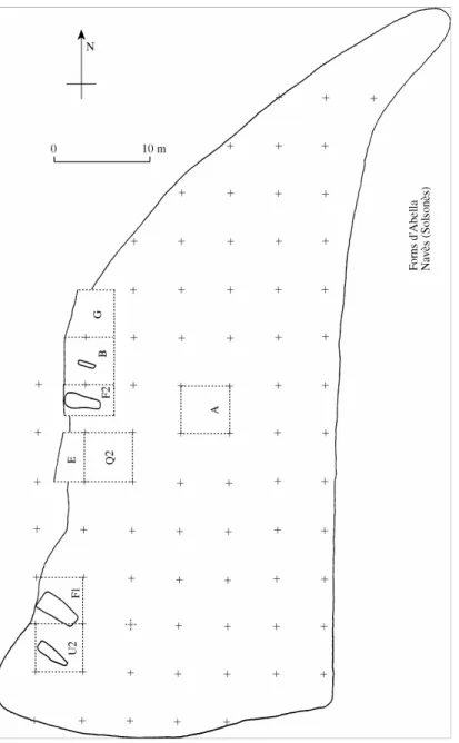
The Abella workshop (Navès, Solsonès) is situated in what is now Catalonia (Spain), in the north-east of the Iberian Peninsula. It constituted the first known workshop of Hispanic Terra Sigillata (Samian Ware). Discovered in 1912, a partial excavation was undertaken by Serra i Vilaró (Serra, 1925) during the first years of this century. As a result of this excavation, three kilns were discovered that belonged to a production centre of Terra Sigillata and common pottery. Moreover, some elements of the kiln were recovered, such as the gas extraction tubes used in irradiation kilns to isolate the firing chamber in order to achieve the completely oxidising atmosphere needed to produce the red Terra Sigillata (Picon, 1973). A new survey led to the discovery of a fourth kiln and a great variety of archaeological materials (Gurt et al., 1987; Gurt, 1993a; Casas et al., 1989; Buxeda, 1995a). The survey was conducted in a number of areas (Figure 1) which correspond to the four kilns (U2, F1, F2 and B) and to a futher four sectors (E, Q2, G and A). The chronology of the workshop was

estimated as being the second half of the 2nd century - first half of the 3rd century AD, thanks to the results provided by the Roman villa of La Rectoria, ca. 500 m away from the workshop, where the Abella products were found in a clear stratigraphical sequence. Also, a 14C dating exists for the UE 7 stratigraphical unit (Gurt, 1993b; Buxeda, 1995a).

Sampling and analytical methods.

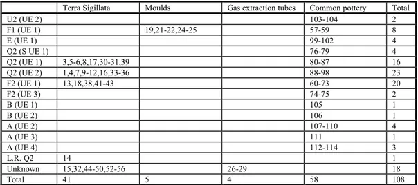
The sampling, conducted in order to define the Abella reference group, included 108 individuals (Table 1), representing the Terra Sigillata, the moulds, the gas extraction tubes and the fine common pottery. All but one individual came from deposition contexts in the areas surveyed in Abella. Only one individual came from the La Rectoria site. However, the deposition context of 18 of the 107 individuals from the Abella site is unknown, because of earlier excavations.

Ten grams of each individual were taken and powdered in a Spex Mixer (Mod. 8000) tungsten carbide cell mill, after the outer surfaces had been mechanically removed. The chemical compositions of the 108 individuals were determined at the Scientific-Technical Services of the University of Barcelona with X-ray Fluorescence (XRF), using a Phillips PW 1400 spectrometer, with two excitation sources: Rh and Au. The quantification of the concentrations was obtained using a calibration line performed with 40 International Geological Standards. The elements determined were: Fe2O3 (as total Fe), Al2O3, MnO, P2O5, TiO2, MgO, CaO, Na2O, K2O, SiO2, Ba, Rb,

Mo, Th, Nb, Pb, Zr, Y, Sr, Sn, Ce, Co, Ga, V, Zn, W, Cu and Ni. The loss on ignition (LOI) was measured by firing 0.5 g, of dried powder, at 1000°C for 1 h. Moreover, X-ray Diffraction analysis (XRD) was carried out for the 108 individuals included in the study, using the same powders prepared for XRF analysis. Measurements were performed at the Scientific-Technical Services of the University of Barcelona using a Siemens D-500 diffractometer working with the Cu K-α radiation (λ=1.5406Å), and monochromator graphite in the diffracted beam, at 1.2 kW (40kV, 30 mA). Spectra were taken from 4 to 70°2Θ, at 1°2Θ/min (step size=0.05°2Θ; time=3 s). Individual 25 was chosen for a thermodiffractometric experiment, using the Siemens D-500 diffractometer equipped with a high temperature chamber and a Positional Sensitive Detector (PSD). Several spectra were taken at room temperature, 600, 700, 750, 800, 850, 900, 950, 1000, 1050 and 1100°C. A rate of 100ºC/h was employed, and the temperature was kept for 1 h before the spectra were recorded. Individuals 1, 3, 6, 11, 13, 18, 24, 25, 26, 28, 29, 31, 32, 46 and 55 were chosen for the study of the microstructure and sintering state presented in its as-received-state (ARS). The observations were made on fresh fracture using a scanning electron microscopy (SEM) Phillips-SEM 515 (Laboratory of Archaeometry, NCSR “Demokritos”, Aghia Paraskevi, Greece), and an SEM Stereoscan S120 (Cambridge Instruments) (Scientific-Technical Services, University of Barcelona). Four individuals (1, 6, 11 and 46) were also refired in oxidising atmosphere, using a rate of 200ºC/h from room temperature up to 850, 950, 1080 and 1100°C, maintaining the temperature for 1 h and with a natural cooling process. A detailed description of the analytical conditions, precision, accuracy, and routine is given by Buxeda (1995a).

As established by Aitchinson (1986), the covariance structure in compositional data for a D-parts composition x is the group of all the covariances

σij,kl=cov{log(xi/xk),log(xj/xl)} (i,j,k,l=1,...,D).

Following this definition for covariance, the variances, representing the relative variations between two components, are defined as

τij=σii,jj=var{log(xi/xj)}.

Furthermore, the covariance structure of a D-parts composition x is actually completely determined by the previous 1/2dD variances. Thus the DxD matrix

T=[τij]=[var{log(xi/xj)}:i,j=1,...,D] (19)

which completely determines the covariance structure is called the variation matrix (Aitchinson, 1986, 1990).

If we develop Aitchinson’s concepts for an S-parts subcomposition applying a logratio transformation, it is clear that given the relation τiS=σii,SS, the values in the

Sth column of the variation matrix are the same as those in the diagonal of the logratio covariance matrix calculated using the component xS as divisor:

ΣΣΣΣ=[σij,SS]=[cov{log(xi/xS),log(xj/xS)} (i,j=1,...,S-1)]. (20)

It has to be pointed out that this correspondence is only partial, because the logratio covariance matrix (20) does not contain the variance τSS, because it contains one

dimension less. Even so, given τSS=0, we can calculate a new value as

τ.S τiS i S = =

∑

which corresponds to the value tr(ΣΣΣΣ), i.e. the total variance in the logratio covariance matrix.

Another important concept arising from the variation matrix (19) is the total variation (Aitchinson, 1990), given by

vt=(2S)-1j'Tj,

where j is the Sx1 column vector of units. This total variation is the measure of the variability existing in the covariance structure for the subcompositional data matrix under study. The importance of the total variation concept is enhanced by the relation between the total variation and the trace of the logratio covariance matrix (20)

vt=tr(ΣΣΣΣ)-S-1j'ΣΣΣΣj,

where j is the (S-1)x1 column of vector units, and therefore vt always assumes a lower value than tr(ΣΣΣΣ). The variation matrix will then allow us to measure the variability linked to the component used as divisor in (11), because the value

vt/τ.S (τ.S=tr(ΣΣΣΣ))

can be considered the percentage of tr(ΣΣΣΣ) explained by the total variation in the covariance structure, the subtraction 1-(vt/τ.S) being the variability imposed on ΣΣΣΣ by

the component xS due to its special role in the asymmetric transformation (11). In this

way, the variation matrix (19) will exhibit in its columns i (i=1,...,S) the diagonals of the S possible logratio matrices that will result when using the component in the ith column as the divisor.

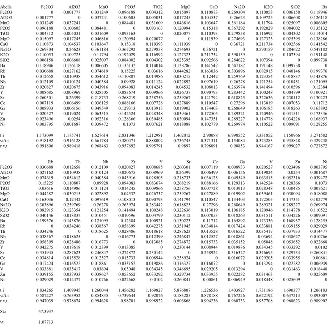
The variation matrix from Abella (Table 2), adapted in accordance with Aitchinson’s proposal, exhibits in its columns the diagonals of all the possible logratio covariance matrices, and the values τ.i (i=1,...,S) (21) corresponding to the traces of

these logratio covariance matrices (Mo, Pb, Sn and Cu are not included due to undeterminations and analytical imprecision; Co, W and LOI will be considered

separately). The total variation is 1.07713. Two groups of elements can be observed. On the one hand, there are some components that, when used as divisors impose a low variability on the transformed data without greatly exceeding the total variation of the covariance structure. The use of SiO2, Y, Fe2O3 and Al2O3 as divisors keeps vt/τ.i

higher than 90%, and therefore they impose a variability below 10%. On the contrary, P2O5, CaO, Ba, K2O, Sr and Na2O give vt/τ.i values below 50%, i.e. they impose a

variability over 50%. These latter values reflect major relative variations between the components used as divisor and the other components determined, which is unexpected in a monogenic sample such as that from Abella. So, the variance matrix shows a covariance structure with a clear influence of these components, indicating their responsibility for most of the existing variability.

When SiO2 is used as divisor in the transformation (11), because it is the

component which imposes least variability, the logratio covariance matrix trace is 1.150966 (value of τ.SiO2). However, the sum of the relative variations of the previous

six components (P2O5, CaO, Ba, K2O, Sr and Na2O) with SiO2 has a value of

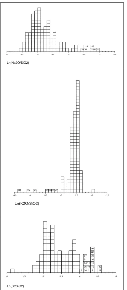
0.898434, i.e. 78.06% of the total variability in the logratio covariance matrix. If we observe, for example, the histograms of the values ln(Na2O/SiO2), ln(K2O/SiO2) and

ln(Sr/SiO2) (Figure 2), we see that some important asymmetries are present. These

asymmetries are unexpected as we assume a normal multivariate distribution function, where a normal univariate must be observed for all the marginal. These asymmetries are at the origin of the high value of the corresponding variances. Furthermore, the highest values in all the variation matrix are observed in relative variations with Na2O,

τSr Na2O and τK2O Na2O, because the individuals involved in these asymmetries are either

the same in opposite directions, or different in the same direction (Figure 2). Finally, it is important to notice that two values appear markedly lower in the column of Sr,

τCaO Sr and τBa Sr.

These results show that the variation matrix is a powerful tool for quantification of the total variation in the compositional data matrix, and also for the identification of the origin of this variability. Certain aspects of this variability can be studied and controlled.

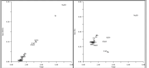
The variability imposed by the component used as divisor in (11) is not the only distortion that this transformation can introduce because of its special role. A second problem arises in the form of distortion of the general behaviour of the components in the covariance structure, a distortion which is due to the relations existing between these components and the component used as divisor. A measure of this distortion can be established with a correlation coefficient rv,τ. between the τji

(j=1,...,i-1,i+1,...,S) values in the ith column and the τ.j (j=1,...,i-1,i+1,...,S) values of

the totals of the other columns, 1 being the value for no distortion. In the case of Abella, the highest correlation is exhibited by the component SiO2, while the lowest is

exhibited by the component Sr. In Figure 3 we can clearly see that the relative variations of all the components with SiO2 are in good agreement with the relative

variations of each component with all the others. On the contrary, the election of Sr as divisor imposes almost 82% of the variability on the logratio covariance matrix, and it also implies a distortion when reproducing the relative variations.

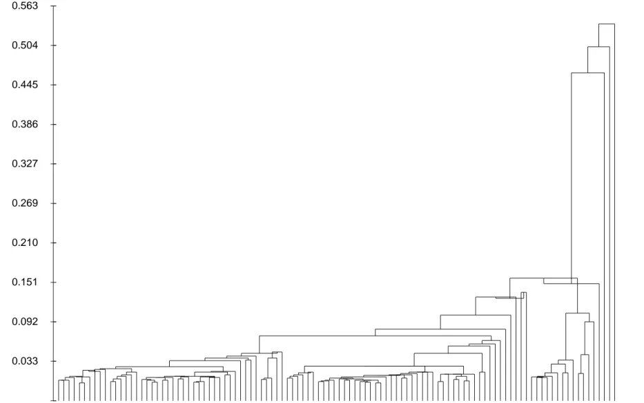
The result of the data treatment can be summarised in the dendrogram of the cluster analysis (Figure 4) performed using the components Fe2O3, Al2O3, MnO, P2O5,

TiO2, MgO, CaO, Na2O, K2O, SiO2, Ba, Rb, Zr, Sr and V, logratio transformed using

SiO2 as divisor. The cluster analysis has been performed, running the program Clustan

(Wishart, 1987), using the mean squared Euclidean distance in order to emphasise the effect of those variables that, after the transformation, present a higher contribution to the variability. The centroid agglomerative algorithm was used because the few reversals do not imply any major transgression of the monotone invariance (Sneath & Sokal, 1973, 278) and, on the contrary, this algorithm has an interesting geometric reflection (Sneath & Sokal, 1973, 234). The value of the cophenetic correlation coefficient is 0.84, which reflects a high hierarchy within the data.

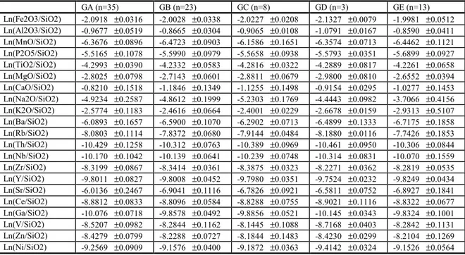
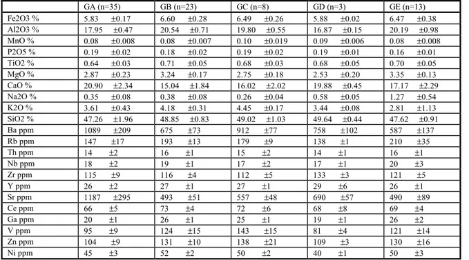
If we centre our attention on what now appears to be more important aspects, we can see a complex structure in the data with 79 out of 108 individuals placed in 4 groups (GA, GB, GC and GE). Table 3 shows the mean and standard deviations for the transformed data in each group, while Table 4 shows the mean and standard deviations for those groups but expressed in normalised subcompositions. In Table 3, we can see that the values ln(Na2O/SiO2) are clearly higher for the group GE, while

the values ln(K2O/SiO2) are much lower. This explains the high value τK2O Na2O,

produced by the two asymmetries in opposite directions but affecting the same individuals, roughly those in the group GE. In relation to the components, CaO, Ba and Sr, we observe that the values ln(CaO/SiO2), ln(Ba/SiO2) and ln(Sr/SiO2) are

markedly higher for group GA, where those individuals involved in the asymmetries exhibited by these three components are grouped. Finally, groups GB and GC represent those individuals not involved in any of these important relative variations. The differences between both groups are less significant, as is reflected in the dendrogram (Figure 4).

The component P2O5, which also makes a major contribution to the

compositional variability, exhibits its special behaviour because of individual 14 (extreme right in the dendrogram) which presents a value of 2.20% in normalised subcompositions while all other values are below 0.37%.

The interpretation of the existing structure.

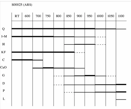
Almost all the individuals exhibit an XRD pattern that can be related to one of the four categories of associations of crystalline phases proposed in Figure 5, according to the observed mineralogical changes. This evolution is supported by the high temperature experiment conducted on individual 25 (Figure 6), which exemplifies mineralogical category C1 in Figure 5, and by the results from SEM on the individuals ARS and the experiments of refiring (Buxeda, 1995a; Buxeda & Cau, 1995a). The equivalent firing temperatures were estimated from the data obtained by XRD and SEM, and can be divided into four groups: below 800-850ºC for C1 (low fired), around 950ºC for C2 (well fired) (crystallisation of gehlenite, pyroxene and plagioclase), between 1000 and 1050ºC for C3 (overfired) (decomposition of illite-muscovite and gehlenite, further development of pyroxene and plagioclase) and over 1100-1150ºC for C4 (severely overfired) (partial decomposition of quartz, crystallisation of leucite) (Maggetti, 1981; Maniatis et al., 1981). It is also important to notice that these results are in good agreement with such indications as the matrix colour (C1, brown or orange depending on the crystallisation of hematite; C2, light orange; C3, yellowish; C4, greenish), and the deformation of some individuals in

category C4, because of the collapse due to the advanced liquid phase produced during firing (Picon, 1973).

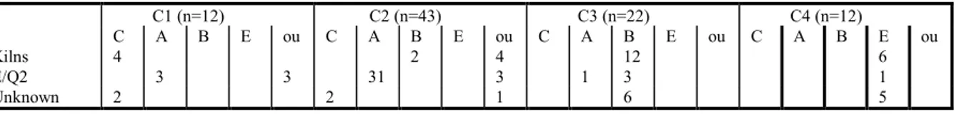
If we exclude the few individuals that must be considered as particular cases, comparison between the chemical and the mineralogical data shows a significant degree of correspondence for 89 out of the 108 individuals retained. In Table 5 we have grouped the individuals, according to their deposition contexts in the site, in three categories: for the individuals coming from the kilns (areas U2, F1, F2 and B in Figure 1), from outside the kilns (areas E and Q2), and for those individuals of unknown deposition context. Thus, we can see that 4 out of 8 individuals of the chemical group GC are classified in mineralogical category C1, with the kilns as their deposition context. For the other 4 individuals of the chemical group GC we do not know the deposition context, but it is worth noting that 2 of them are classified in mineralogical category C1 and the other 2 are classified in mineralogical category C2. The correspondence between these data is still clearer for the individuals of the chemical group GA, in which 31 out of the 35 individuals are classified in mineralogical category C2 and come from the deposition contexts outside the kilns. The other 4 individuals grouped in GA also come from the same deposition context, but they are classified in mineralogical categories C1 (3 individuals) and C3 (1 individual), which are the mineralogical categories next to C2. In the case of the chemical group GB, 21 out of 23 individuals are classified in mineralogical category C3. Nevertheless, no relation is observed in this case between chemical group GB and a specific deposition context. Only 2 individuals of the chemical group GB are classified in mineralogical category C2, but they come from deposition contexts outside the kilns. Finally, 12 out of 13 individuals of the chemical group GE are classified in mineralogical category C4. As in the previous chemical group, no relation is observed between chemical group GE and a specific deposition context.

It can then be clearly observed that the structure in several chemical groups, provoked by the existence of several asymmetries involving certain individuals, is linked to the firing temperature (to the physical, mineralogical and chemical characteristics developed by the firing) and to the deposition context. The reason for this is the presence of selective alteration and contamination processes. In this sense, the values ln(CaO/SiO2), ln(Ba/SiO2) and ln(Sr/SiO2) reflect the perturbation

operating on the components CaO, Ba and Sr (Figure 7). In the case of ln(CaO/SiO2),

these values are related to the crystallisation of secondary calcite (for example, Heimann & Maggetti, 1981; Maggetti et al., 1984; Picon, 1985a), which would imply a partial enrichment with allochthonous Ca2+. Notwithstanding, the phenomenon of secondary calcite is a very complex problem which needs the concurrence of more than one analytical technique for its identification, and especially for its interpretation in terms of enrichment with allochthonous calcium. In the case of Abella, the data support such an interpretation (vid., Buxeda & Cau, 1995a). In relation with the values ln(Ba/SiO2) and ln(Sr/SiO2), contaminations of Ba and Sr have also been reported (for

example, Bieber, 1977; Olin et al., 1978; Freestone et al., 1985; Picon, 1985b; Picon, 1987; Schmitt, 1989; Béarat, 1990; Picon, 1991). In the case of Abella, the data suggest the existence of a certain association between the contamination of calcium, barium and strontium, especially affecting those individuals in mineralogical categories C1 and C2, that are buried in the deposition contexts E/Q2.

In Figure 8 we can observe the asymmetries detected in mineralogical category C4. In this fabric we can observe the effect of two different, possibly partially related, processes that cause the contamination of sodium and the lixiviation of potassium, perhaps because of the alteration of the glassy phase (for example, Picon, 1976; Segebade & Lutz, 1980; Lemoine et al., 1981; Schmitt, 1989; Picon, 1991). This lixiviation is not observed in all the individuals in category C4, but, what has to be taken into consideration is that all the individuals in this category present, with different intensities, peaks of leucite, a potash feldspatoid (Figure 5 and Figure 6). This firing phase could act as a way of fixing the potassium, preventing its lixiviation. On the contrary, what is made clear is the contamination of sodium for all the individuals. In this case, this contamination of sodium is directly related to the crystallisation of a sodium zeolite, analcime (Figure 5), which is clearly a secondary phase (for example, Maggetti, 1981; Heimann & Maggetti, 1981; Walter, 1988). This process is also possibly favoured by the alteration of the glassy phase. The analcime was semiquantified on the basis of the intensity in counts per second (CPS) of its peak 5.59Å. The diagram analcime-ln(Na2O/SiO2) shows the relation between the presence

of analcime and the sodium content.

Moreover, it should be pointed out that individual 14, which can be classified in mineralogical category C2 and which has markedly the highest observed variability in P2O5, is the only individual from the La Rectoria site. In contrast to the production

site of Abella, La Rectoria was an inhabited Roman villa that was used as a cemetery during the Medieval Ages. This may have given rise to the relation between this contamination and the organic matter on the site. However, none of our data directly support this identification, that is the phase where the phosphorous is fixed, or the mechanism of its formation (Buxeda, 1995a).

Finally, cobalt and tungsten, not considered in the previous discussion, are typical examples of alterations and contaminations produced in the laboratory. Here, the use of a tungsten carbide cell mill is the cause of these contaminations. If we recalculate the variation matrix including these two components, we obtain a value vt/τ.Co of 50.53%, where the contribution of the total variation to the logratio

covariance matrix is as low as 50%. In the case of tungsten, the value vt/τ.W is

significantly lower, 9.41%. These results were expected because cobalt is a minor element in the composition of the cell, while tungsten is a major one. Furthermore, it is important to notice that the lowest value in the column of W is τCo W, this reflects

the relationship between both components in the composition of the cell and the parallel occurrence in this contamination (for a similar problem see Attas et al., 1984).

The distribution function.

The Abella case shows that the perturbing vector is a function of three wide groups of variables (Buxeda, 1995a):

u=f(F,E,t),

where F is the fabric (which includes the chemistry, the mineralogy, the structural characteristics, etc. for the individuals, and which is the result of the transformations during firing of the initial paste), E is the environment (i.e. any environment in which the ceramic was placed during use, burial, etc.; it includes chemistry, pH, temperature,

etc.), and t is time (the duration of the contact between the ceramic and a special environment with stable or changing conditions). In the present example, the variables ‘association of crystalline phases obtained by XRD’ and ‘deposition context in the site’ operate as simply two very rough estimates of fabric and environment, respectively.

If the component used as divisor is always directly operated by the neutral element, the use of logratio transformed data retains the effect of the perturbations within the components directly perturbed. It also allows the original ratios (i.e. the original distances) to be recovered between those components of different individuals directly operated by the neutral element. With this procedure, we avoid the estimation of the values of the components of the perturbing vector u (Aitchinson, 1986), which in practice is almost impossible (Woronow & Love, 1990). This control over indirect operations is important in defining the reference group when estimating mean (16), variance (17) and covariance (18), because the effect of the perturbations is kept within the directly perturbed components. Therefore, when we define the distribution function, if this is a normal multivariate, as

NS-1(µµµµ,ΣΣΣΣ),

where we consider only the subcomposition of the S elements as always being directly operated by the neutral element, we recover the original distribution function for this subcomposition.

Final implications: loss on ignition and tempering.

The data treatment derived from transformation (11) allows us to control a difficult problem, the loss on ignition (LOI) value. The LOI value incorporates several terms: the volatile elements (Cogswell et al., 1996) and, especially, certain elements such as hydrogen, oxygen and carbon that are usually not determined and that are related to the organic matter, the compositional water of primary phases and anions such as CO32-, which are present in the original paste. This process, which is not a

perturbation operation as defined in this paper, can actually be modelled as a perturbation induced by firing temperature during the transformation process from paste to fabric. Therefore, the logratio transformation also allows us to control the effect of this paste-to-fabric change, and the diversification of compositions with the apparent dilution effect for the determined concentrations (Kilikoglou et al., 1988).

If we recalculate the variation matrix of Table 2, taking into consideration the LOI, we obtain a value vt/τ.LOI of 15.41%, and values clearly lower in column LOI for

the variances τCaO LOI, τBa LOI and τSr LOI. These results were expected because the

alterations and contaminations affecting the enrichment in calcium, barium and strontium are observed in the individuals classified in mineralogical categories C1 and C2, which correspond to the lowest firing temperatures. The means in raw data of the LOI are (in %) GC 10.31 (± 2.08), GA 8.71 (± 2.41), GB 4.15 (± 1.08), and GE 3.21 (± 1.63), which show the dramatic effect of the indirect operations induced by LOI.

This model can also be applied to tempering. The tempering problem has been extensively discussed in the literature as the dilution problem imposed by the decrease in concentrations for the determined elements when the temper is added (Neff et al.,

1988; Neff et al., 1989; Beier & Mommsen, 1994). If we take the raw material as a compositional vector and the temper as a perturbing one, the addition of temper has two effects: 1) through the direct operation it changes the original concentrations of those components operated by values other than the neutral element (all values are uj>1, except uj=1 when the corresponding element is not present in the temper), and 2)

through the indirect operation being divided by k (4), due to the constraining operator of compositional data, which affects all the components independently of the direct operation. For example, quartz temper affects trace element determinations through the indirect operation. Thus, it is clear that what has been called an inert diluent does not actually exist (Neff et al., 1989). What does exist, however, are cases in which the direct perturbation affects only undetermined components. In this sense, we can see that the logratio transformation can deal with the so-called dilution problem.

As an example, if we repeat the cluster analysis in Figure 4, without including the components ln(P2O5/SiO2), ln(CaO/SiO2), ln(Na2O/SiO2), ln(K2O/SiO2),

ln(Ba/SiO2) and ln(Sr/SiO2) in the subcomposition used, the present structure

disappears. Individual 14, affected by the contamination in P2O5, is also placed

amongst the other individuals. The lower ultrametric distances reflect large reduction in the variability. Also, some new differences are now apparent having previously been obscured by the perturbations dominating the data treatment, and in particular it appears that individuals 108 and 109 exhibit a quite distinct chemical composition. The most interesting point is that individual 87, a clear outlier in Figure 4, is now placed among all the individuals. This fact is important if we consider that this individual is the only one that presents a low calcareous clay (in normalised subcomposition the CaO is 2.99%). This result clearly shows that using the logratio transformation in the appropriate way we can avoid differences such as calcium content, which can be changed by the potter through the addition of temper, thus recovering the original values in raw materials.

Conclusions.

The study of chemical data from Abella kiln material has allowed us to identify a high compositional variability, particularly for certain components. Comparing chemical and mineralogical data, as well as physical properties, has made the interpretation of the compositional variability, insofar as it is related to alteration and contamination processes, possible. These processes have affected the individuals differently, because of the fabric and the deposition context.

The advantages of using the logratio transformation rather than the centred logratio are clear theoreticallu, since the asymmetric transformation is more robust when facing the perturbations. The logratio transformation highlights the existence of compositional variability, perhaps imposed by perturbation operations, through the variances in the variation matrix. It also allows the indirect perturbation to be avoided, by dividing the data in (11) with a component that is not directly perturbed, as well as the direct perturbation by excluding the directly perturbed components in the data treatment. In this way, the unknown original distances and distribution functions are recovered for the subcomposition of the determined components which are not directly perturbed.

Notwithstanding, if what we face is the need to explain mathematically the compositional variability of the chemical characterisation, this explanation implies certain assumptions that cannot be demonstrated in the mathematical solution itself. Thus, the explanation of the compositional variability requires the identification and interpretation as perturbation (including alteration and contamination processes, LOI, tempering and technology) or as polygenic provenance (Buxeda, 1995b). Furthermore, the interpretation and explanation of this compositional variability requires the use of data other than chemical, and also the concurrence of validation archaeological data.

To achieve these objectives, the logratio transformation proposed by Aitchinson has been found to be the most appropriate, and it is robust enough to allow the use of all the determined components since initially they have equal value, which ought to be the only assumption allowed during the data treatment (Sneath & Sokal, 1973).

Acknowledgements.

This study is the result of a postdoctoral fellowship funded by the Catalan Autonomous Government at the Laboratoire de Céramologie, UPR 7524, CNRS, Lyon (France). The author is indebted to the Director Dr. M. Picon who has contributed highly useful suggestions. The analyses were undertaken at the Scientific-Technical Services (University of Barcelona), within Dr. J.M. Gurt i Esparraguera’s research project PB92-0851 funded by the DIGICYT (Spanish Government), and some SEM work was carried out at the Laboratory of Archaeometry, NCSR “Demokritos”, Aghia Paraskevi (Greece). The author is also indebted to Dr. V. Kilikoglou for his enthusiasm and willingness to discuss this work, and to Dr. M.A. Cau Ontiveros for his work and for his constant comments on the contents of this paper. The author would finally like to thank Mr. A. Nikolaidis for revising the English text.

Bibliography.

Aitchinson, J. (1986). The Statistical Analysis of Compositional Data. London: Chapman and Hall.

Aitchinson, J. (1989). Reply to “Interpreting and Testing Compositional Data” by Alex Woronow, Karen M. Love, and John C. Butler. Mathematical Geology

21, 65-71.

Aitchinson, J. (1990). Relative Variation Diagrams for Describing Patterns of Compositional Variability. Mathematical Geology 22, 487-511.

Aitchinson, J. (1992). On Criteria for Measures of Compositional Difference. Mathematical Geology 24, 365-379.

Arnold, D.E. (1992). Comments on Section II. In (H. Neff, Ed.) Chemical Characterisation of Ceramic Pastes in Archaeology. Monographs in World Archaeology, 7. Madison, Wisconsin: Prehistory Press, pp. 107-134.

Attas, M., Fossey, J.M. & Yaffe, L. (1984). Corrections for drill-bit contamination in sampling ancient pottery for Neutron Activation Analysis. Archaeometry 26, 104-107.

Baxter, M.J. (1989). Multivariate analysis of data on glass compositions: a methodological note. Archaeometry 31, 45-53.

Baxter, M.J. (1991). Principal Component Analysis of glass compositions: an empirical study. Archaeometry 33, 29-41.

Baxter, M.J. (1992). Statistical analysis of chemical compositional data and comparison of analyses. Archaeometry 34, 267-277.

Baxter, M.J. (1993). Comment on D. Tangri and R.V.S. Wright, "Multivariate analysis of compositional data...". Archaeometry 35(1)(1993). Archaeometry

35, 112-115.

Baxter, M.J. (1994). Exploratory multivariate analysis in Archaeology. Edinburgh: Edinburgh University Press.

Béarat, H., Dufournier, D., Nguyen, N., Raveau, B. (1989). Influence de NaCl sur le coleur et la composition chimique des pâtes céramiques au cours de leur cuisson. Revue d’Archéométrie 13, 43-53.

Béarat, H. (1990). Étude de quelques altérations physico-chimiques des céramiques archéologiques. Thèse de Doctorat. Caen: Université de Caen.

Beier, T. & Mommsen, H. (1994). Modified Mahalanobis filters for grouping pottery by chemical composition. Archaeometry 36, 287-306.

Bieber, A.M. (1977). Neutron activation analysis of archaeological ceramics from Cyprus. Ph.D. dissertation. Ann Arbor, Michigan: University of Connecticut. Bieber, A.M. Jr., Brooks, D.W., Harbottle, G. & Sayre, E.V. (1976). Application of

multivariate techniques to analytical data on Aegean ceramics. Archaeometry

18, 59-74.

Buxeda i Garrigós, J. (1995a). La caracterització arqueomètrica de la ceràmica de Terra Sigillata Hispanica Avançada de la ciutat romana de Clunia i la seva contrastació amb la Terra Sigillata Hispanica d'un centre productor contemporani, el taller d'Abella. Col.lecció de Tesis Doctorals Microfitxades

2524. Barcelona: Universitat de Barcelona.

Buxeda i Garrigós, J. (1995b). Problemas en torno a la variación composicional. In Monográfica Arte y Arqueología. Granada: Universidad de Granada (in press). Buxeda i Garrigós, J. & Cau Ontiveros, M.A. (1995a). Identificación y significado de

la calcita secundaria en cerámicas arqueológicas. Complutum 6, 293-309. Buxeda i Garrigós, J. & Cau Ontiveros, M.A. (1995b). Alteration in punic amphorae

from Ebussus (Evissa, Balears). 4th Meeting “Weathering processes in ceramics and stone artefacts during burial” (NATO CCMS-Cultural Technologies). Lisbon.

Buxeda i Garrigós, J. & Gurt i Esparraguera, J.M. (1995). Problemas para el establecimiento del grupo de referencia del taller de Abella: perturbaciones en el patrón. Trabalhos de Antropologia e Etnologia 35, 471-481.

Buxeda i Garrigós, J., Cau Ontiveros, M.A., Gurt i Esparraguera, J.M. & Tuset i Bertran, F. (1995). Análisis tradicional y análisis arqueométrico en el estudio de las cerámicas comunes de época romana. In Ceràmica comuna romana d’època alto-imperial a la Península Ibèrica. Estat de la qüestió, Monografies Emporitanes VIII. Empúries: Conjunt Monumental d’Empúries, pp. 39-60. Casas, A., Pinto, V., Gurt i Esparraguera, J.M., Riera i Mora, S. & Burés i Vilaseca, L.

(1989). Aplicación de la prospección magnética en la localización de hornos de cerámica romana en Navès (Lleida). In S.F.E.C.A.G., Actes du Congrés de Lezoux (mai, 1989). Marseille, pp. 169-174.

Cogswell, J.W., Neff, H. & Glascock, M.D. (1996). The Effect of Firing Temperature on the Elemental Characterisation of Pottery. Journal of Archaeological Science 23, 283-287.

Cuomo di Caprio, N. (1985). La ceramica in archeologia, antiche tecniche di lavorazione e moderni metodi d'indagine. Ed. La Fenice: Roma.

Dufournier, D. (1982). L’utilisation de l’eau de mer dans la preparation des pâtes céramiques calcaires. Premières observations sur les conséquences d’un tel traitement. Revue d’Archéométrie 6, 87-100.

Duma, G. (1972). Phosphate content of ancient pots as indication of use. Current Anthropology 13, 127-130.

Freestone, I.C., Meeks, N.D. & Middleton, A.P. (1994). Retention of phosphate in buried ceramics: an electron microbeam approach. Archaeometry 27, 161-177. Freeth, S.J. (1967). A chemical study of some bronze age pottery sherds.

Archaeometry 10, 104-119.

Gurt i Esparraguera, J.M. (1993a). Pla d'Abella, Navès. In Annuari d'intervencions arqueològiques 1982-1989. Epoca romana, Antiguitat Tardana. Campanyes 1982-1989. Col.lecció Annuaris d'Intervencions Arqueològiques a Catalunya

1. Barcelona: Generalitat de Catalunya, p. 217.

Gurt i Esparraguera, J.M. (1993b). La Rectoria, Navès. In Annuari d'intervencions arqueològiques 1982-1989. Epoca romana, Antiguitat Tardana. Campanyes 1982-1989. Col.lecció Annuaris d'Intervencions Arqueològiques a Catalunya

1. Barcelona: Generalitat de Catalunya, p. 218.

Gurt i Esparraguera, J.M., Miret, M. & Xandri, J. (1987). Dades sobre la romanització a la comarca del Solsonès (Lleida). In Pre-actes de les Jornades Internacionals d'Arqueologia Romana. Granollers, pp. 39-44.

Heimann, R.B. & Maggetti, M. (1981). Experiments on simulated burial of calcareous Terra Sigillata (mineralogical change). Preliminary results. In (M.J. Hughes, Ed.) Scientific Studies in Ancient Ceramics. British Museum Occasional Paper

19. London, pp. 163-177.

Hoard, R.J., Holen, S.R., Glascock, M.D. & Neff, H. (1995). Additional Comments on Neutron Activation Analysis of Stone from the Great Plains: Reply to Church. Journal of Archaeological Science 22, 7-10.

Kilikoglou, V., Maniatis, Y. & Grimanis, A.P. (1988). The effect of purification and firing of clays on trace element provenance studies. Archaeometry 30, 37-46. Leese, M., Hughes, M.J. & Stopford, J. (1989). The chemical composition of tiles

from Bordesley: a case study in data treatment. In (S. Rahtz & J. Richards, Eds.) Computer applications and quantitative methods in archaeology. Int. Ser., S548. Oxford: B.A.R., pp. 241-249.

Lemoine, C., Meille, E., Poupet, P., Barrandon, J.N. & Borderie, B. (1981). Étude de quelques altérations de composition chimique des céramiques en milieu marin et terrestre. Revue d’Archéométrie Suppl. S, 349-360.

Maggetti, M. (1981). Composition of Roman pottery from Lousonna (Switzerland). In (M.J. Hughes, Ed.) Scientific studies in ancient ceramics. British Museum Occasional Paper, 19. London, pp. 33-49.

Maggetti, M., Westley, H. & Olin, J.S. (1984). Provenance and technical studies of Mexican majolica using elemental and phase analysis. In (J.B. Lambert, Ed.) Archaeological Chemistry III. Advances in Chemistry Series 205. Washington D.C.: American Chemical Society, pp. 151-191.

Maniatis, Y., Simopoulos, A., Kostikas, A. (1981). Moessbauer Study of the Effect of Calcium Content on Iron Oxide Transformations in Fired Clays. Journal of the American Ceramic Society 64, 263-269.

Matson, F.R. (1971). A study of temperature used in firing ancient Mesopotamian pottery. In (R.H. Brill, Ed.) Science and Archaeology. Cambridge, Massachusetts: The MIT Press, pp. 65-79.

Millet, A. (1967). In (J.F. Bass) Cape Gelidonya: a bronze age shipwreck. Philadelphia.

Morel, J.-P. & Picon, M. (1995). Les céramiques étrusco-campaniennes: recherches en laboratoire. In (G. Olcese, Ed.) Ceramica romana e archaeometria. Lo stato degli studi. Firenze: C.N.R., Museo Archeologico e della Ceramica di Montelupo, Ed. all’Insegna del Giglio, pp. 23-46.

Neff, H., Bishop, R.L. & Sayre, E.V. (1988). A Simulation Approach to the Problem of Tempering in Compositional Studies of Archaeological Ceramics. Journal of Archaeological Science 15, 159-172.

Neff, H., Bishop, R.L. & Sayre, E.V. (1989). More observations on the Problem of Tempering in Compositional Studies of Archaeological Ceramics. Journal of Archaeological Science 16, 57-69.

Neff, H. (1994). RQ-Mode Principal Component Analysis of Ceramic Compositional Data. Archaeometry 36, 115-130.

Olin, J.S., Harbottle, G. & Sayre, E.V. (1978). Elemental compositions of Spanish and Spanish-colonial majolica ceramics in the identification of provenience. In (G.F. Carter, Ed.) Archaeological Chemistry II. Advances in Chemistry Series

171. Washington D.C.: American Chemical Society, pp. 200-229.

Picon, M. (1973). Introduction à l'étude technique des céramiques sigillées de Lezoux. Centre de Recherches sur les Techniques Gréco-romaines, 2. Dijon: Université de Dijon.

Picon, M. (1976). Remarques préliminaires sur deux types d'altération de la composition chimique des céramiques au cours du temps. Figlina 1, 159-166. Picon, M. (1985a). À propos de l’origine des amphores massaliètes: méthodes et

résultats. Documents d’Archéologie Méridionale 8, 119-131.

Picon, M. (1985b). Un exemple de pollution aux dimensions kilométriques: la fixation du baryum par les céramiques. Revue d’Archéométrie 9, 27-29.

Picon, M. (1986). Analyse de céramiques de l'épave Culip IV et corrections d'altérations. Archéonautica 6, 116-119.

Picon, M. (1987). La fixation du baryum et du strontium par les céramiques. Revue d’Archéométrie 11, 41-47.

Picon, M. (1991). Quelques observations complémentaires sur les altérations de composition des céramiques au cours du temps: cas de quelques alcalins et alcalino-terreux. Revue d’Archéométrie 15, 117-122.

Picon, M. (1992). L'analyse chimique des céramiques: bilan et perspectives. In (R. Francovich, Ed.) Archeometria della Ceramica. Problemi di Metodo. Bologna: Ed. Int. Centro Ceramico, pp. 3-26.

Sayre, E.V., Chan, L.A. & Sabloff, J.A. (1971). High-Resolution Gamma Ray Spectroscopic Analyses of Mayan Fine Orange Pottery. In (R.H. Brill, Ed.) Science and Archaeology. Cambridge, Massachusetts: The MIT Press, pp. 165-181.

Schmitt, A. (1989). Méthodes géochimiques, pétrographiques, et minéralogiques appliquées à la détermination de l’origine des céramiques archéologiques. Thèse de Doctorat. Bordeaux: Université de Bordeaux III.

Segebade, C. & Lutz, G.J. (1980b). Photon activation analysis of ancient Roman pottery. In (E.A. Slater & J.O. Tate, Eds.) Proceedings of the 16th

International Symposium on Archaeometry and Archaeological Prospection (Edimbourgh, 1976). National Museum of Antiquities of Scotland, pp. 20-49. Serra i Vilaró, J. (1925). Cerámica en Abella, primer taller de "terra sigillata"

descubierto en España. Memoria número 73. Madrid: Junta Superior de Excavaciones y Antigüedades.

Sneath, P.H.A. & Sokal, R.R. (1973). Numerical Taxonomy. The Principles and Practice of Numerical Classification. San Francisco: W.H. Freeman & Co.. Steponaitis, V.P. (1984). Technological studies of prehistoric pottery from Alabama:

physical properties and vessel function. In (S.E. van der Leeuw & A.C. Pritchard, Eds.) The Many Dimensions of Pottery. Ceramics in Archaeology and Anthropology. Cingula VII. Amsterdam: Universiteit van Amsterdam, Albert Egges van Giffen Instituut voor Pre-en Protohistoire, pp. 79-122.

Tangri, D. & Wright, R.V.S. (1993). Multivariate analysis of compositional data: applied comparisons favour standard principal component analysis over Aitchinson's loglinear contrast. Archaeometry 35, 103-112.

Tite, M.S. & Maniatis, Y. (1975). Examination of ancient pottery using the Scanning Electron Microscope. Nature 257, 122-123.

Walter, V. (1988). Étude pétrographique, minéralogique et géochimique d’amphores gauloises découvertes dans le Nord-Est de la France. Thèse de Doctorat. Strasbourg: Université des Sciences Humaines de Strasbourg, U.F.R. des Sciences Historiques, CNRS - Centre de Sédimentologie et de Géochimie de la Surface.

Weigand, P.C., Harbottle, G. & Sayre, E.V. (1977). Turquoise sources and source analysis: Mesoamerica and the Southwestern U.S.A.. In (T.K. Earle & J.E. Ericson, Eds.) Exchange systems in prehistory. Academic Press Inc.: New York & London, pp. 15-34.

Widemann, F., Picon, M., Asaro, F., Michel, H.V. & Perlman, I. (1975). A Lyons branch of the pottery-making firm of Ateius of Arezzo. Archaeometry 17, 45-59.

Wishart, D. (1987). Clustan User Manual. Edinburgh: Computing Laboratory, University of St. Andrews.

Whitbread, I.K. (1989). A proposal for the systematic description of thin sections towards the study of ancient technology. In (Y. Maniatis, Ed.) Archaeometry. Proceedings of the 25th International Symposium (held in Athens from 19 to 23 May 1986). Amsterdam: Elsevier, pp. 127-138.

Woronow, A. & Love, K.M. (1990). Quantifying and Testing Differences Among Means of Compositional Data Suites. Mathematical Geology 22, 837-854.

Terra Sigillata Moulds Gas extraction tubes Common pottery Total U2 (UE 2) 103-104 2 F1 (UE 1) 19,21-22,24-25 57-59 8 E (UE 1) 99-102 4 Q2 (S UE 1) 76-79 4 Q2 (UE 1) 3,5-6,8,17,30-31,39 80-87 16 Q2 (UE 2) 1,4,7,9-12,16,33-36 88-98 23 F2 (UE 1) 13,18,38,41-43 60-73 20 F2 (UE 3) 74-75 2 B (UE 1) 105 1 B (UE 2) 106 1 A (UE 2) 107-110 4 A (UE 3) 111 1 A (UE 4) 112-114 3 L.R. Q2 14 1 Unknown 15,32,44-50,52-56 26-29 18 Total 41 5 4 58 108

Table 1. Sampling undertaken at Abella, according to ceramic class and deposition context. L.R.: La Rectoria site. Unknown: unknown deposition context.