Advantages of using a fast urban boundary layer model as
compared to a full mesoscale model to simulate the urban heat
island of Barcelona
Markel García-Díez1, Dirk Lauwaet2, Hans Hooyberghs2, Joan Ballester1,4, Koen De Ridder2, and Xavier Rodó1,3,4
1Institut Català de Ciències del Clima, Barcelona, Catalonia, Spain 2VITO, Antwerp, Belgium
3Institució Catalana de Recerca i estudis Avançats (ICREA), Barcelona, Catalonia, Spain
4Climate and Health Program, ISGlobal, Barcelona Institute for Global Health, Barcelona, Catalonia, Spain
Correspondence to:Markel García-Díez ([email protected])
Received: 13 January 2016 – Published in Geosci. Model Dev. Discuss.: 9 February 2016 Revised: 26 October 2016 – Accepted: 27 October 2016 – Published: 8 December 2016
Abstract. As most of the population lives in urban envi-ronments, the simulation of the urban climate has become a key problem in the framework of the climate change im-pact assessment. However, the high computational power required by high-resolution (sub-kilometre) fully coupled land–atmosphere simulations using urban canopy parame-terisations is a severe limitation. Here we present a study on the performance of UrbClim, an urban boundary layer model designed to be several orders of magnitude faster than a full-fledged mesoscale model. The simulations are evalu-ated with station data and land surface temperature obser-vations from satellites, focusing on the urban heat island (UHI). To explore the advantages of using a simple model like UrbClim, the results are compared with a simulation car-ried out with a state-of-the-art mesoscale model, the Weather Research and Forecasting Model, which includes an urban canopy model. This comparison is performed with driving data from ERA-Interim reanalysis (70 km). In addition, the effect of using driving data from a higher-resolution fore-cast model (15 km) is explored in the case of UrbClim. The results show that the performance of reproducing the aver-age UHI in the simple model is generally comparable to the one in the mesoscale model when driven with reanalysis data (70 km). However, the simple model needs higher-resolution data from the forecast model (15 km) to correctly reproduce the variability of the UHI at a daily scale, which is related to the wind speed. This lack of accuracy in reproducing the wind speed, especially the sea-breeze daily cycle, which is strong in Barcelona, also causes a warm bias in the reanalysis
driven UrbClim run. We conclude that medium-complexity models as UrbClim are a suitable tool to simulate the urban climate, but that they are sensitive to the ability of the input data to represent the local wind regime. UrbClim is a well suited model for impact and adaptation studies at city scale without high computing requirements, but does not replace the need for mesoscale atmospheric models when the focus is on the two-way interactions between the city and the at-mosphere
1 Introduction
According to the United Nations, more than 50 % of the world population lives in cities, and this percentage is ex-pected to increase in the coming decades. The urban en-vironment is known to modify the local climate in several different ways. The most well known is the so-called ur-ban heat island (UHI) effect, which causes temperatures to be several degrees higher over the urban area in compari-son to its rural surroundings. Due to anthropogenic climate change, the frequency of heat waves is expected to undergo a widespread increase (Meehl and Tebaldi, 2004) in the fol-lowing decades. This raises concerns about the vulnerabil-ity of people living in urban areas. Although the magni-tude of the UHI effect does not necessarily increase due to global warming (Lauwaet et al., 2015), it has been shown to be large enough to potentially have significant impacts. The
most important ones are human health, through heat stress (Gabriel and Endlicher, 2011; Dousset et al., 2011) and en-ergy consumption (Kikegawa et al., 2006; Kolokotroni et al., 2012).
The physical causes of the UHI effect were enumerated by Oke (1982), but the relative contribution of each one is still discussed. Zhao et al. (2014) used satellite observations and a model simulation to calculate the relative contribu-tion of the different causes of the UHI in 65 cities of North America. They considered contributions from modifications in the radiative balance, evaporation, convection efficiency, heat storage and anthropogenic heat sources. They found that the relative contribution of these factors depends on the local background climate of the city and on the time of the day. In general, during daytime, convection efficiency and evapo-transpiration are the main drivers of the UHI, while heat stor-age is the most relevant during the night. Zhao et al. (2014) used satellite-retrieved land surface temperatures, but these can differ from screen level temperatures. Others have high-lighted the complexity of the problem of measuring the UHI, given that it is difficult to monitor the urban climate with enough detail and reliability (Arnfield, 2003). Furthermore, the complexity of the urban surface, featuring anisotropy and vertical surfaces, makes it complicated to sample by satellites (Voogt and Oke, 1998). These difficulties with the observa-tions increase the value of numerical simulaobserva-tions, which can produce detailed fields that are not observable. At the same time, the lack of observations hampers the evaluation of these simulations.
Recently, urban canopy models or parameterisations have been included in many regional climate models (RCMs) (see. for example Huszar et al., 2014, and Ching, 2013). RCMs are limited area models used, among many other applica-tions, to dynamically downscale climate change projections from coarse resolution global circulation models. Neverthe-less, computational power limitations do not allow RCMs to reach the level of resolution that is required to resolve most of the cities. Here we study, by using a simplified model that only accounts for the Planetary Boundary Layer (PBL) and the surface physics, the possibility of reaching resolu-tions of 250 m with affordable computational resources. This model, called UrbClim, has been developed by De Ridder et al. (2015), and is described in Sect. 2.3. UrbClim has been already evaluated in a few European cities (De Ridder et al., 2015; Zhou et al., 2015; Lauwaet et al., 2016) and used to generate climate change projections (Lauwaet et al., 2015). Note that UrbClim has a different, more specific scope than the RCMs, being focused on the fast and computationally light simulation of the UHI and the heat stress in the ur-ban environment, so that it can be easily transferred between cities. While this scope covers many applications, it must be mentioned that RCMs are required to reproduce the two-way interaction between the city and the atmosphere affecting the rain, storm initiation and other phenomena, at the expense of a much larger computational cost.
Statistical downscaling can also be considered as an al-ternative (or complementary) methodology to assess the ur-ban climate. However, statistical downscaling is observation-dependent, and spatially detailed observations at a city scale covering long periods are very rare. UrbClim, instead, al-lows for long multi-decadal adaptation experiments where changes in the city surface parameters can be tested (e.g. the colour of the roofs or the evaluation of the effects that changes in construction materials in building may have). The main aim of this model is to simulate only the fundamental processes that cause the UHI, so that the model is lightweight but still based on physics, thus allowing sensitivity experi-ments to be conducted.
In the present paper, we evaluate UrbClim over the city of Barcelona, and compare it with a standard mesoscale model, the Weather Research and Forecasting Model (WRF), us-ing an urban canopy parameterization. Namely, the sus-ingle layer urban canopy model (SLUCM) was used, which was developed by Kusaka et al. (2001) and coupled to WRF by Chen et al. (2011). It has been verified in several studies (Lee et al., 2011) and used for future climate change projections (Argüeso et al., 2015; Georgescu et al., 2014; Kusaka et al., 2012).
Barcelona is located in the Euro-Mediterranean region, which has been defined as a primary climate change hotspot (Giorgi, 2006), as it emerges as an especially responsive area to climate change, with more frequent, longer and harsher summer heat waves (Meehl and Tebaldi, 2004; Ballester et al., 2009, 2010a, b). Taking into account that the Mediter-ranean countries are currently more vulnerable to environ-mental summer conditions than other European societies, the larger magnitude of the projected temperature increase is expected to become a major challenge for public health in summer (Ostro et al., 2012). For example, the negative ef-fects of the record-breaking 2003 heat wave in central and southern Europe were particularly damaging in the Euro-Mediterranean region (Robine et al., 2008). The seasonal mortality excesses were indeed similar in Spain (13.7 %), France (11.8 %) and Italy (11.6 %), although temperature anomalies were twice as large in France than in the southern countries (Ballester et al., 2011). This larger sensitivity to environmental conditions is exacerbated by urban pollution and especially affects old people, living in cities, with pre-existing or chronic cardiovascular and respiratory diseases (McMichael et al., 2006).
Taking into account all these considerations, the city of Barcelona emerges as a particularly vulnerable area within the continent. Barcelona is located in northeastern Spain, sur-rounded by the Mediterranean Sea in the south and east, a small 500 m mountain range in the northwest, and two rivers in the southwest and northeast (Fig. 1, and see also Fig. 2 for the location of the urbanised area). Its Mediterranean climate (Csa in the Köppen classification) is shaped in summer by the local wind breeze regime, whose diurnal evolution exhibits a clockwise rotation from southerlies in the morning to winds
Figure 1. (a) Topography of the UrbClim domain and locations of the meteorological stations. The two stations used as a reference of the urban and rural climates are highlighted with red stars. (b) Three WRF domain edges (red squares) and UrbClim domain edges (black contour), together with the topography of the WRF domains with 10, 3.3 and 1.1 km resolution.
blowing roughly parallel to the southwest–northeast shore-line in the late afternoon (Redaño et al., 1991). The main goals of the paper are:
– Evaluation of a UrbClim simulation of the urban cli-mate in the city of Barcelona, driven by reanalysis data at 70 km resolution, against station and satellite data. – Comparison, both in terms of model skill and
compu-tational resources, of the UrbClim simulation against a benchmark simulation performed with a state-of-the art mesoscale model, driven with the same reanalysis data. – Analysis of the sensitivity of the UrbClim simulation to the boundary conditions, comparing the original run against a simulation driven by a higher-resolution fore-cast dataset (15 km).
2 Data and methodology 2.1 Surface stations
As a first approach in the evaluation of the model perfor-mance, we have used data from a set of meteorological sta-tions, four of them belonging to the Spanish Meteorological Agency (AEMET) and seven to the Catalan Meteorological Service (SMC). Both data providers carry out quality control on this data before distributing them. All are well maintained automatic stations that deliver meteorological data with 10 or 20 min frequency. In the present work, only hourly data were used. The locations of these stations, as well as their names, are displayed in Fig. 1a, together with the topography.
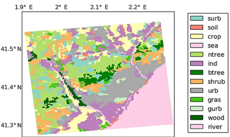
Station number 5 (El Prat de Llobregat) is chosen to be representative of a rural location near the city. This station is surrounded by cereal fields (Fig. 2), located 300 m from the Llobregat river and 650 m from the closest urban area.
Sta-Figure 2. Distribution of the land-use types used in the UrbClim simulations, which were derived from the CORINE dataset.
tion number 6 (el Raval) is instead chosen as the reference ur-ban station. This station is located on the roof of a building in the city centre of Barcelona, 8.5 km away from the rural sta-tion. Pictures for the locations of both el Raval1and el Prat2 stations are available on the website of the SMC. These two points are almost the closest possible rural–urban points lo-cated at a similar height. The rural station is at 8 m above sea level, while the urban station is at 33 m, which can account for a difference of 0.15–0.25◦C difference in a standard at-mospheric profile. The rural station is located in a delta, and therefore the surrounding topography is flat, with no rele-vant orographic objects between the two stations. Thus, the differences between these two stations are considered to be representative of the UHI effect in the city of Barcelona. 2.2 Satellite data
The spatial pattern of the simulations is evaluated through data from the Moderate Resolution Imaging Spectroradiome-ter (MODIS) of the National Aeronautics and Space Admin-istration (NASA) of the United States. Following previous works (Schwarz et al., 2011; Zhou et al., 2015), MODIS datasets MOD11A2 and MYD11A2 (version 5) were down-loaded and processed. These correspond to the Terra and Aqua satellites respectively, and are 8-day aggregations of the daily MOD11A1 and MYD11A1 datasets, using only the clear-sky days. The variable considered is land surface temperature (LST), which is derived from the infrared ra-diance and emissivity estimated from land-cover types. A more detailed description of the algorithms is available in Wan (2008).
The LST data were processed considering only the data flagged as “good quality, not necessary to examine more de-tailed QA” (quality assessment) in the Quality Flag provided with the data, and with no cloudy days during the 8-day pe-riod. This introduces a bias for certain meteorological
con-1http://www.meteo.cat/observacions/xema/dades?codi=X4 2http://www.meteo.cat/observacions/xema/dades?codi=XL
ditions (clear-sky days), which is unavoidable. MODIS and UrbClim LST data were interpolated to a 0.01◦regular grid
for direct comparison. Finally, only the images with less than 14 % missing values were used (this percentage does not in-clude the data over the sea which are always missing). The days (and the times of the day) considered in the averages are the same in the model data and in the observations. The 8-day averages flagged as containing cloudy days in MODIS were masked before computing the averages in both sides. This process left a total of 15 values for most grid points (Fig. S1 in the Supplement) over the whole period.
2.3 The UrbClim model
The UrbClim model is designed to simulate the temperature and heat-stress fields at a city scale with a minimum amount of computational power, so that it is possible to perform long runs at a resolution of hundreds of metres. A detailed descrip-tion of the model is available in De Ridder et al. (2015). Urb-Clim models the lower 3 km of the atmosphere, and consists of a 3-D boundary layer model and land–surface scheme with urban physics. As in mesoscale models, the boundary data is imposed from a lower-resolution model, but the boundary conditions scheme differs somewhat. Apart from the vari-ables usually fed to the mesoscale models, UrbClim also needs the radiative fluxes and the precipitation. Instead of using a relaxation zone, UrbClim imposes the driving model data in the inflow boundary points, and a “zero gradient” con-dition, which lets the perturbations flow outside the domain, in the outflow points.
Mesoscale models develop their own variability and struc-tures with respect to the lower-resolution models driving them, which is called internal variability (Giorgi and Bi, 2000). By design, UrbClim does produce a significantly smaller internal variability than a mesoscale model. This can be considered as a disadvantage, as it does not permit study of the full two-way interaction of the city with the regional troposphere. But, on the other hand, it is the key for saving computational power. As the UHI is rooted in the surface properties and the heat storage in the ground, using a model like UrbClim is reasonable. This model does work approxi-mately as a wind tunnel, without creating regional structures in the atmospheric flow, so it is possible to nest it directly in much lower-resolution models without creating intermediate nests. Nonetheless, this resolution jump can affect the qual-ity of the simulation if the driving model does not accurately reproduce the local climate. Mesoscale models need these in-termediate nests so that the inconsistencies between internal variability and driving data do not affect the numerical sta-bility. This trade-off between the internal variability and the computational efficiency will be key for the interpretation of the results in this study.
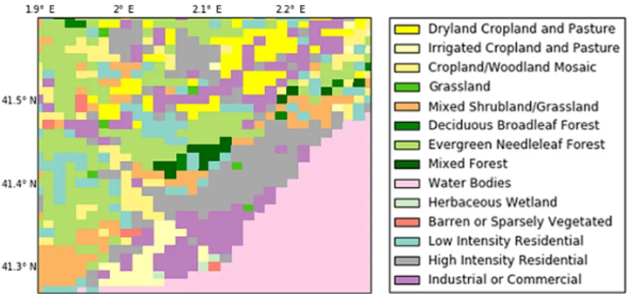
Figure 3. Distribution of the land-use types used in the WRF simulation. They were mapped from the CORINE dataset to the USGS classes.
The land-use data, which are needed to represent the sur-face properties, are taken from the CORINE dataset3. This dataset is publicly available online, and was produced by the European Environmental Agency at a resolution of 100 m. Figure 2 shows the distribution of the land-use classes used by UrbClim.
The land-surface scheme is a standard soil–vegetation– atmosphere model based on Ridder and Schayes (1997), which was extended to fully account for the urban canopy. This updated version is described in detail in De Ridder et al. (2015). The 3-D boundary layer model represents a simplified atmosphere by using the conservation equations for the horizontal momentum, potential temperature, spe-cific humidity and mass. The turbulent vertical diffusion is represented following Hong and Pan (1996). The urban physics use an urban slab, together with a parameterization of the inverse Stanton number. This simple approach is jus-tified in De Ridder et al. (2015), because the heat coeffi-cients can be taken from real-world experiments, rather than the scale experiments that the more detailed urban canopy models use to get the transfer coefficients of walls, roofs and roads. In contrast, the single-layer urban canopy model (SLUCM) included in WRF represents simple symmetrical street canyons with infinite length (Kusaka et al., 2001). It is important to note that the goal of the present study is not no compare this UCM with the one used by UrbClim, but the whole WRF–SLUCM modelling system. Thus, the dif-ferences found between WRF and UrbClim are not necessar-ily related to the different approximations used to represent the Urban Canopy.
2.4 Experimental setup 2.4.1 UrbClim
The UrbClim simulations cover the five warmest months of year 2011, i.e. from May to September. The domain is rep-resented by a horizontal grid with 121 × 121 points at a
res-3http://www.eea.europa.eu/publications/COR0-landcover
olution of 250 m, with 19 vertical levels within the 3 lower km of the troposphere (Fig. 1a). The driving model data are updated every 3 h. Two simulations have been studied, la-belled as UC-ERA and UC-FC. The former is driven by the ERA-Interim reanalyses (Dee et al., 2011), while the latter is driven by the Integrated Forecasting System (IFS) ver-sion 37r2 global forecast model of the European Centre for Medium-Range Weather Forecasts (ECMWF). In 2011, this model ran with a spectral resolution of T1279 (' 15 km), in contrast with the T255 (' 70 km) of ERA-Interim. Thus, it is able to provide more local details, which can be impor-tant given the aforementioned mesoscale-driven weather of Barcelona.
2.4.2 WRF
The Weather Research and Forecasting model is an open-source, non-hydrostatic limited area model (Skamarock et al., 2008). Thanks to its availability, it has a large commu-nity of users. These contribute to the development of WRF, which is lead by the National Center for Atmospheric Re-search (NCAR). One particularity of this model is that it has a large amount of parameterization schemes, dynamical op-tions and sub-modules, available for the user to choose from. These options are set up in a namelist file that must be edited for each simulation.
In the present study, we used the version 3.6.1 of WRF, which was configured to run in three nested domains (Fig. 1b), with 40 vertical levels and horizontal resolutions of 10, 3.3 and 1.1 km. The 250 m of UrbClim were not reached because the computational cost was not affordable. However, the simulations were carefully configured to make them com-parable with UrbClim: they were nested in the same dataset (ERA-Interim) and used the same land use (CORINE). WRF land use is taken by default from the United States Geologi-cal Survey (USGS) dataset. Thus, the CORINE land classes were mapped to the USGS 33 classes following Table 7.1 of Chrysoulakis et al. (2014). The resulting land-use class map is shown in Fig. 3.
0 5 10 15 20 Time (UTC) 18 20 22 24 26 28 Te m pe ra tu re (C ◦) Urban OBS WRF UC-ERA UC-FC 0 5 10 15 20 Time (UTC) 18 20 22 24 26 28 Te m pe ra tu re (C ◦) Rural OBS WRF UC-ERA UC-FC 0 5 10 15 20 Time (UTC) 2 1 0 1 2 3 Te m pe ra tu re u rb an - ru ra l ( C ) ◦ Urban - rural OBS WRF UC-ERA UC-FC
Figure 4. Average daily temperature cycle in the urban (left) and rural (middle) stations. The difference urban minus rural is shown in the panel on the right. The “UC-ERA”, “UC-FC” and “WRF” legend codes are defined in Sect. 2, while “OBS” represents the observation.
Despite being nested in a reanalysis, the regional models tend to generate their own internal variability. While this is necessary to the RCM to add value, it is not convenient to let the model to drift too much from the reanalyses, as these in-corporate observations and are accurate descriptions of past atmospheric states. There are two approaches to solving this: using nudging, or restarting the model frequently. In this case, based on the experience of previous studies (Menendez et al., 2014; García-Díez et al., 2015), daily 36 h simulations have been carried out and concatenated, leaving 12 h as spin-up. These simulations cover the same time span as UrbClim, from May to September 2011. Thus, 153 individual simu-lations have been carried out. To handle them, the WRF4G framework (Fernández-Quiruelas et al., 2015) has been used.
3 Results 3.1 Time series
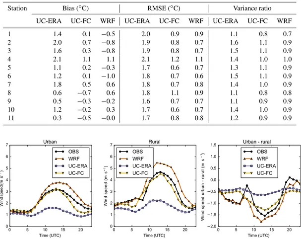
Table 1 shows scores of daily mean 2 m temperature for the UC-ERA, UC-FC and WRF simulations and the 11 stations. The largest errors are found in UC-ERA, which generally overestimates daily temperatures by up to +2◦C at some stations. This overestimation is associated with the misrepre-sentation of the sea breeze, which has a larger effect on max-imum temperatures. This is discussed later in the manuscript. UC-ERA also overestimates the day-to-day variability, hav-ing higher root mean square error (RMSE) than the other runs. Instead, UC-FC and WRF show similar, smaller scores, which indicate the good performance of these simulations.
Figure 4 shows the average daily cycles for the urban and rural stations, as well as their difference. The average mag-nitude of the UHI during the night is found to be 2.5◦C, which is large enough to have direct impacts on human health during heat wave episodes (Ye et al., 2012). During day-time hours, the UHI is found to decrease down to −0.5◦C. Note that this is in very close agreement with the values rived from observational data in Moreno-García (1994), de-spite using two different reference points. The measurement
of the UHI with only two points has some limitations, as it may be sensitive to very local features such as the land use in the vicinity of the stations. However, the representative-ness of these points has been carefully checked with high-resolution satellite images. In addition, the agreement with previous studies increases our confidence in the results here presented.
UC-ERA tends to overestimate temperatures at both sta-tions after 10:00 UTC and particularly during daytime hours, but errors in both stations cancel each other, and therefore the UHI magnitude is generally well represented with biases smaller than 0.5◦C. The UHI average daily cycle is similar in UC-FC and UC-ERA, but UC-FC does not show any warm bias, and accurately reproduces the observed temperatures of the individual stations.
In the case of WRF, we initially considered the nearest grid point to the rural and urban stations, and biases in the three panels were found to be clearly larger than those in Ur-bClim (not shown). This problem was found to be related to the land use of the grid points, which were not representative of the land use of the stations. Indeed, the grid point repre-senting the rural station was found to be classified as urban in the land cover map used by WRF. In order to address this problem, we considered a more representative, adjacent grid point to represent the rural station, which is used through-out the paper (see Figs. S1 and S2 in the Supplement for the details). Results show that biases in WRF for the individual stations are large and negative throughout the day except in the evening, but comparable in magnitude to those in UC-ERA. In addition, although the UHI at noon is correctly re-produced by WRF, its bias is clearly larger at 07:00 (−1.5◦C) and 17:00 UTC (−1◦C).
Regarding the wind speed (Fig. 5), the intensity of the sea breeze is clearly underestimated in UC-ERA, with a bias of up to −2.5 m s−1 at noon in the rural station. This problem is likely to be related with the coarse resolution of the ERA-Interim driving dataset, which is not able to resolve the sharp daytime, thermally driven pressure gradient between the con-tinent and the sea. The lack of sea breeze in turn explains the
2 2.0 0.7 −0.8 1.9 0.8 0.7 1.6 1.1 0.9 3 1.6 0.3 −0.8 1.9 0.8 0.7 1.5 1.1 0.9 4 2.1 1.1 1.1 2.1 1.2 1.1 1.4 1.0 1.0 5 1.1 0.2 −0.3 1.7 0.6 0.7 1.3 1.1 0.9 6 1.2 0.1 −1.0 1.8 0.7 0.6 1.5 1.1 0.9 7 1.8 0.5 0.6 1.8 0.7 0.8 1.4 1.0 0.9 8 0.6 −0.7 0.6 1.8 1.1 0.9 1.1 0.8 0.8 9 0.5 −0.3 −0.2 1.6 0.7 0.7 1.1 0.9 0.9 10 1.2 −0.2 0.3 1.7 0.6 0.7 1.4 1.0 0.9 11 0.3 −0.5 −0.0 1.7 0.8 0.8 1.2 0.9 0.9 0 5 10 15 20 Time (UTC) 0 1 2 3 4 5 6 7 W in d sp ee d (m s ) − 1 Urban OBS WRF UC-ERA UC-FC 0 5 10 15 20 Time (UTC) 0 1 2 3 4 5 6 7 W in d s p e e d ( m s − 1) Rural OBS WRF UC-ERA UC-FC 0 5 10 15 20 Time (UTC) 2.0 1.5 1.0 0.5 0.0 0.5 1.0 1.5 W in d s p e e d ur b a n ru ra l (m s ) − 1 Urban - rural OBS WRF UC-ERA UC-FC
Figure 5. Same as Fig. 4, but for wind speed.
nearly constant daily cycle of the rural-minus-urban differ-ence in wind speed in UC-ERA. The wind regime is clearly better reproduced in the other simulations. UC-FC accurately reproduces the daily wind cycle in both the urban and rural stations, while WRF overestimates the wind speed by up to 1 m s−1 during daytime hours. Regarding the urban-minus-rural difference, WRF is the model that better captures the hourly evolution of the wind speed. UC-FC correctly simu-lates the overall magnitude of the difference, but it is not able to reproduce the secondary minima and maxima at 06:00 and 08:00 UTC.
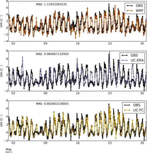
It is interesting to highlight the day-to-day variability of the observed and simulated times series for the month of May (Fig. 6). The whole period is not shown for clarity, but the same conclusions are applicable for the other months. The daily evolution of the UHI is well represented in UC-FC and WRF, while biases of the order of up to 4◦C at noon are found in UC-ERA for some specific days. How-ever, the largest mean absolute error (MAE) is found in WRF (1.11◦C), due to the systematic underestimation of the UHI during daytime hours (Fig. 4). This underestimation is small,
albeit persistent. The best MAE score is found in UC-FC (0.80◦C), which shows regular skill with almost no large er-rors in specific days.
From these results, it is clear that the performance of Urb-Clim is largely improved as a result of the higher resolution of the ECMWF forecast model compared to ERA-Interim (15 km vs. 70 km). It is, however, unclear how to understand the comparison of WRF with UrbClim. On the one hand, UC-ERA and WRF, which are both nested in the same reanaly-ses, display comparable scores regarding the magnitude of the UHI, although WRF better represents the wind speed and some spatio-temporal features of temperature. On the other hand, WRF performs a full dynamical downscaling down to a resolution of 1.1 km, and therefore, in principle it should be able to achieve an accuracy similar to UC-FC. But, as we have shown, UC-FC exhibits better scores than WRF. Given the large number of factors involved, it is difficult to find an explanation to this result in physical terms. In general, WRF is more biased than UC-FC (Figs. 4, 5 and 6) and than the ECMWF forecast itself (not shown). It tends to underesti-mate temperatures and to overestiunderesti-mate the wind speed during
Figure 6. Hourly time series of the 2 m temperature difference between the urban and the rural locations for May 2011, for WRF (top), UC-ERA (middle) and UF-FC (bottom).
the day. As WRF is very customisable, it could be possible, in principle, to find a configuration that removes these biases. However, WRF biases in wind speed are found to be difficult to correct, and research is yet ongoing in this line (García-Díez et al., 2015; Lorente-Plazas et al., 2016).
3.2 Spatial pattern
The evaluation of the spatial variability simulated by the ur-ban climate model is a challenging issue due to the lack of reliable, high-resolution observations. Figure 7 shows the av-erage daily minimum temperatures for UC-ERA, UC-FC and WRF, for the five months considered. Although both models are able to resolve the main features of the UHI of Barcelona, the surrounding cities and the airport, the UrbClim run at a resolution of 250 m provides much more detailed informa-tion, e.g. a clear representation of the hill to the southwest of the city centre. ERA is generally warmer than UC-FC, due to the misrepresentation of winds, but the spatial patterns are very similar. In addition, the temperature differ-ence is similar in the urban and rural sites. Unfortunately, the scarcity of surface observations did not allow us to evaluate
the spatial patterns at the screen level, and therefore we eval-uated the spatial variability of the model by analysing the MODIS satellite LST, as described in Sect. 2.2.
During the night, both UC-ERA and WRF have been found to overestimate LST over urban areas, and therefore also the LST UHI (Fig. 8). This is surprising, given the small error found in the evaluation of the screen level UHI. Other studies (Zhou et al., 2015) found small errors when com-paring MODIS and UrbClim LST in and around the city of London. As mentioned in the introduction, measuring LST over urbanised areas is challenging, due to the uncertainties associated with the measurement of both the radiation and the emissivity. By comparing modelled (panels b and c) and observed (panel a) maps in Fig. 8, it can be seen that the bias outside the urban areas is found to be relatively small in WRF, and slightly negative in UC-ERA, while the spatial patterns are reasonably similar between the models and the satellite data. Determination of emissivity over urban areas is notoriously difficult and subject to large uncertainties, which could explain at least part of model deviation of LST. The spatial Pearson correlations between the observed and
sim-Figure 7. Daily minimum temperature averaged over the period May–September 2011 in (a) UC-ERA, (b) UC-FC and (c) WRF.
Figure 8. Land surface temperature averaged during nighttime hours over the period May–September 2011 in MODIS (left), UC-ERA (cen-tre) and WRF (right).
ulated fields are 0.77 ± 0.025 for UC-ERA and 0.70 ± 0.03 for WRF, where the confidence bounds were computed with bootstrapping (1000 samples). Thus, the spatial correlation in UC-ERA is higher, and the difference is statistically sig-nificant. However, taking into account the above-mentioned differences in the bias, we conclude that the performance of the spatial pattern in WRF and UC-ERA are comparable.
It is worth mentioning that the MODIS LST appears to have an effective resolution coarser than 1 km, given that the spatial patterns are smooth and do not resolve many detailed features. Finally, as mentioned in the introduction, LST and surface air temperature (SAT) UHIs are not equivalent, and are driven by different phenomena. Thus, it is also possible that models that reproduce the SAT UHI correctly generate at the same time a biased LST UHI.
3.3 Computational resources
In this section, the computational resources required by Ur-bClim and WRF are compared. The comparison is not fully trivial because UrbClim does not currently support running in parallel, which can be seen as an important drawback. However, UrbClim does not require a long spin-up, and therefore the simulations can be parallelised just by splitting the time period in subperiods and running the corresponding simulations simultaneously in different machines or nodes.
For a direct comparison, both models were run in the local cluster of the Institut Català de Ciències del Clima (IC3), while the main UrbClim runs used in the paper were carried out in the VITO cluster. The IC3 cluster
is made of 48 homogeneous server blades, having each of them two “quad core” processors, 48 GB of mem-ory, 146 GB of disk space and fast network interconnect (Infiniband). The blade model is Sun Blade X6270 (see http://www.oracle.com/us/products/servers-storage/servers/ blades/sun-blax6270-m2-ds-080923.pdf for a full de-scription) equipped with Xeon (Nehalem) X5570 processors. Results are summarised in Table 2. With these settings, a WRF simulation of 36 h took 2.5 h to finish (using an average of 10 simulations), including the preprocess carried out with the WRF preprocessor (WPS). This preprocess was run in serial, in 1 core, while WRF was run in 16 cores (that is, two blades). Thus, the total serial equivalent wall-time was 40 h, assuming perfect scaling (the real value will be somewhat below). WRF was compiled using the Intel fortran compiler version 14.0.1 with the Intel MPI Library for Linux OS, Version 4.1 Update 3.
Regarding UrbClim, for this test, it has been compiled with the same compiler and run in the same cluster. A 36 h simulation with UrbClim took 0.3 h to finish (average of 10 simulations) running in one core. Thus, UrbClim running at 250 m resolution is found to be 133 times faster than WRF at 1 km resolution. This enables downscaling large climate change ensembles for a big collection of cities.
Note that the UrbClim speed is not only explained by the smaller number of grid points (Table 2), but especially be-cause of the simplicity of the dynamical core, and the smaller number of parameterisations, compared to WRF.
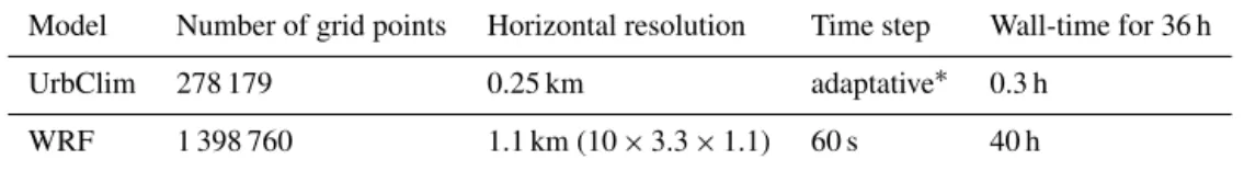
Table 2. Summary of the results of the benchmarking. The number of grid points represents the total number of grid points in the model domain, which is 121 · 121 · 19 in UrbClim, and 100 · 80 · 40 + 136 · 112 · 40 + 121 · 97 · 40 in case of WRF (taking into account the three nested domains).
Model Number of grid points Horizontal resolution Time step Wall-time for 36 h UrbClim 278 179 0.25 km adaptative∗ 0.3 h
WRF 1 398 760 1.1 km (10 × 3.3 × 1.1) 60 s 40 h
∗20 s for the soil scheme and adaptative for the atmosphere, using the Courant–Friedrichs–Lévy stability criterion.
4 Conclusions
In the present work, we have evaluated the performance of a boundary-layer urban climate model (UrbClim) for the warm season in the city of Barcelona. We were particularly in-terested in the study of the UHI effect, given that it rep-resents a major source of health problems in summer for vulnerable people living in urban environments (e.g. heat stress, temperature-related mortality, pollution, vector-borne diseases). We have compared this model (UC-ERA) with the output of a regional climate model (WRF), and analysed the effect of the model resolution in the driving simulation (UC-ERA vs. UC-FC). All these simulations have been evaluated against observations from meteorological stations and satel-lite data (MODIS), in order to analyse the temporal and spa-tial variability of the UHI effect, respectively.
The main conclusions of our work can be summarised as follows:
– The average UHI in the city of Barcelona during the warm season (May–September) reaches 2.5◦C at night. This is relevant for the study of climate impacts, given that it increases the stress on the vulnerable population and for the health care systems under extreme condi-tions.
– UrbClim correctly reproduces the UHI of Barcelona when it is nested to the coarse dataset of ERA-Interim, while it suffers from a general warm bias. When it is nested to a higher-resolution model (ECMWF IFS), UrbClim additionally reproduces well the temperature evolution of the individual rural and urban stations used for the calculation of the UHI.
– WRF is less biased than the UrbClim run nested in ERA-Interim, and both runs show comparable skill in reproducing the UHI.
– The spatial pattern of LST is similar in UrbClim and WRF, even though significant biases are found in both models when they are evaluated against MODIS data. In conclusion, UrbClim has been found to be well suited for the numerical description of the UHI of Barcelona, pro-viding an accurate description of the temperature field. The choice between UrbClim and WRF for the simulation of the
urban environment largely depends on the type of variable and process that is to be analysed. WRF has the advantage of providing a more detailed and complete description of at-mospheric winds and rainfall, which is required in some ap-plications (e.g. pollutant dispersion, urban effect in rainfall). On the other hand, UrbClim has been proven to be as accu-rate as WRF at reproducing the UHI of Barcelona during the warm season, and several orders of magnitude faster. This opens the door to the performance of multi-decadal simula-tions of urban heat stress in a large number of cities at a rea-sonable computational cost, using scenario and multi-GCM ensembles to account for uncertainty, and testing for urban adaptation scenarios.
We found that, in cities affected by strong mesoscale flows (e.g. sea breeze) such as Barcelona, it must be taken into ac-count that UrbClim will be subject to inaccuracies caused by the misrepresentation of the wind, in case that it is nested in a low-resolution model.
Note that this is a specific problem in Barcelona, given that it has not been found in other European cities where Ur-bClim, driven by ERA-Interim, has been successfully tested (De Ridder et al., 2015; Lauwaet et al., 2016; Zhou et al., 2015). From these results, it is reasonable to infer that the skill of UrbClim, and probably of other similar urban bound-ary layer models, is constrained by the performance of the driving model, and particularly for variables that are impor-tant for the UHI such as wind speed and cloudiness.
5 Code and data availability
The UrbClim source code is not publicly available. In order to access it, a specific agreement needs to be signed with VITO. Please contact [email protected] for more details. The WRF model is an open source model, and its code is freely available upon registra-tion at http://www2.mmm.ucar.edu/wrf/users/download/get_ source.html. Weather station data from the Catalan and Spanish meteorological agencies are available for research purposes upon request to [email protected] and https: //sede.aemet.gob.es/AEMET/es/GestionPeticiones/home re-spectively. MODIS data were downloaded from the “Re-verb” NASA tool http://reverb.echo.nasa.gov, where it is freely available upon registration. The CORINE land cover
Acknowledgements. The work described in this paper has received funding from the European Community’s 7th Framework Pro-gramme under Grant Agreements No. 308299 (NACLIM) and 308291 (EUPORIAS). J. Ballester gratefully acknowledges funding from the European Commission through a Marie Curie International Outgoing Fellowship (project MEMENTO from the FP7-PEOPLE-2011-IOF call), and from the European Commission and the Catalan Government through a Marie Curie–Beatriu de Pinós Fellowship (project 00068 from the BP-DGR-2014-B call). Edited by: J. Kala
Reviewed by: three anonymous referees
References
Argüeso, D., Evans, J. P., Pitman, A. J., and Luca, A. D.: Effects of City Expansion on Heat Stress under Cli-mate Change Conditions, PLOS ONE, 10, e0117066, doi:10.1371/journal.pone.0117066, 2015.
Arnfield, A. J.: Two decades of urban climate research: a review of turbulence, exchanges of energy and water, and the urban heat island, Int. J. Climatol., 23, 1–26, doi:10.1002/joc.859, 2003. Ballester, J., Douville, H., and Chauvin, F.: Present-day
clima-tology and projected changes of warm and cold days in the CNRM-CM3 global climate model, Clim. Dynam., 32, 35–54, doi:10.1007/s00382-008-0371-0, 2009.
Ballester, J., Giorgi, F., and Rodó, X.: Changes in European tem-perature extremes can be predicted from changes in PDF central statistics, Climatic Change, 98, 277–284, doi:10.1007/s10584-009-9758-0, 2010a.
Ballester, J., Rodó, X., and Giorgi, F.: Future changes in Central Europe heat waves expected to mostly follow summer mean warming, Clim. Dynam., 35, 1191–1205, doi:10.1007/s00382-009-0641-5, 2010b.
Ballester, J., Robine, J.-M., Herrmann, F. R., and Rodó, X.: Long-term projections and acclimatization scenarios of temperature-related mortality in Europe, Nat. Commun., 2, 358, doi:10.1038/ncomms1360, 2011.
Chen, F., Kusaka, H., Bornstein, R., Ching, J., Grimmond, C. S. B., Grossman-Clarke, S., Loridan, T., Manning, K. W., Martilli, A., Miao, S., Sailor, D., Salamanca, F. P., Taha, H., Tewari, M., Wang, X., Wyszogrodzki, A. A., and Zhang, C.: The integrated WRF/urban modelling system: development, evaluation, and ap-plications to urban environmental problems, Int. J. Climatol., 31, 273–288, doi:10.1002/joc.2158, 2011.
Ching, J. K. S.: A perspective on urban canopy layer modeling for weather, climate and air quality applications, Urban Climate, 3, 13–39, doi:10.1016/j.uclim.2013.02.001, 2013.
P., Kobayashi, S., Andrae, U., Balmaseda, M. A., Balsamo, G., Bauer, P., Bechtold, P., Beljaars, A. C. M., van de Berg, L., Bid-lot, J., Bormann, N., Delsol, C., Dragani, R., Fuentes, M., Geer, A. J., Haimberger, L., Healy, S. B., Hersbach, H., Hólm, E. V., Isaksen, L., Kållberg, P., Köhler, M., Matricardi, M., McNally, A. P., Monge-Sanz, B. M., Morcrette, J.-J., Park, B.-K., Peubey, C., de Rosnay, P., Tavolato, C., Thépaut, J.-N., and Vitart, F.: The ERA-Interim reanalysis: Configuration and performance of the data assimilation system, Q. J. Roy. Meteor. Soc., 137, 553–597, doi:10.1002/qj.828, 2011.
Dousset, B., Gourmelon, F., Laaidi, K., Zeghnoun, A., Giraudet, E., Bretin, P., Mauri, E., and Vandentorren, S.: Satellite monitoring of summer heat waves in the Paris metropolitan area, Int. J. Cli-matol., 31, 313–323, doi:10.1002/joc.2222, 2011.
Fernández-Quiruelas, V., Fernández, J., Cofiño, A. S., Blanco, C., García-Díez, M., Magariño, M., Fita, L., and Gutiérrez, J. M.: WRF4G: WRF experiment management made simple, Geosci. Model Dev. Discuss., 8, 6551–6582, doi:10.5194/gmdd-8-6551-2015, 2015.
Gabriel, K. M. and Endlicher, W. R.: Urban and rural mortality rates during heat waves in Berlin and Brandenburg, Germany, Envi-ron. Pollut., 159, 2044–2050, doi:10.1016/j.envpol.2011.01.016, 2011.
García-Díez, M., Fernández, J., San-Martín, D., Herrera, S., and Gutiérrez, J.: Assessing and Improving the Local Added Value of WRF for Wind Downscaling, J. Appl. Meteorol. Clim., 54, 1556–1568, doi:10.1175/JAMC-D-14-0150.1, 2015.
Georgescu, M., Morefield, P. E., Bierwagen, B. G., and Weaver, C. P.: Urban adaptation can roll back warming of emerging megapolitan regions, P. Natl. Acad. Sci. USA, 111, 2909–2914, doi:10.1073/pnas.1322280111, 2014.
Giorgi, F.: Climate change hot-spots, Geophys. Res. Lett., 33, L08707, doi:10.1029/2006GL025734, 2006.
Giorgi, F. and Bi, X.: A study of internal variability of a re-gional climate model, J. Geophys. Res., 105, 29503–29521, doi:10.1029/2000JD900269, 2000.
Hong, S.-Y. and Pan, H.-L.: Nonlocal Boundary Layer Ver-tical Diffusion in a Medium-Range Forecast Model, Mon. Weather Rev., 124, 2322–2339, doi:10.1175/1520-0493(1996)124<2322:NBLVDI>2.0.CO;2, 1996.
Huszar, P., Halenka, T., Belda, M., Zak, M., Sindelarova, K., and Miksovsky, J.: Regional climate model assessment of the urban land-surface forcing over central Europe, Atmos. Chem. Phys., 14, 12393–12413, doi:10.5194/acp-14-12393-2014, 2014. Kikegawa, Y., Genchi, Y., Kondo, H., and Hanaki, K.:
Im-pacts of city-block-scale countermeasures against ur-ban heat-island phenomena upon a building’s energy-consumption for air-conditioning, Appl. Energ., 83, 649–668, doi:10.1016/j.apenergy.2005.06.001, 2006.
Kolokotroni, M., Ren, X., Davies, M., and Mavrogianni, A.: Lon-don’s urban heat island: Impact on current and future energy
consumption in office buildings, Energ. Buildings, 47, 302–311, doi:10.1016/j.enbuild.2011.12.019, 2012.
Kusaka, H., Kondo, H., Kikegawa, Y., and Kimura, F.: A Simple Single-Layer Urban Canopy Model For Atmospheric Models: Comparison With Multi-Layer And Slab Models, Bound.-Lay. Meteorol., 101, 329–358, doi:10.1023/A:1019207923078, 2001. Kusaka, H., Hara, M., and Takane, Y.: Urban Climate Projection by the WRF Model at 3-km Horizontal Grid Increment: Dynamical Downscaling and Predicting Heat Stress in the 2070’s August for Tokyo, Osaka, and Nagoya Metropolises, J. Meteorol. Soc. Jpn. II, 90B, 47–63, doi:10.2151/jmsj.2012-B04, 2012.
Lauwaet, D., Hooyberghs, H., Maiheu, B., Lefebvre, W., Driesen, G., Van Looy, S., and De Ridder, K.: Detailed Urban Heat Island Projections for Cities Worldwide: Dynamical Down-scaling CMIP5 Global Climate Models, Climate, 3, 391–415, doi:10.3390/cli3020391, 2015.
Lauwaet, D., De Ridder, K., Saeed, S., Brisson, E., Chatterjee, F., van Lipzig, N. P. M., Maiheu, B., and Hooyberghs, H.: Assess-ing the current and future urban heat island of Brussels, Urban Climate, 15, 1–15, doi:10.1016/j.uclim.2015.11.008, 2016. Lee, S.-H., Kim, S.-W., Angevine, W. M., Bianco, L., McKeen,
S. A., Senff, C. J., Trainer, M., Tucker, S. C., and Zamora, R. J.: Evaluation of urban surface parameterizations in the WRF model using measurements during the Texas Air Quality Study 2006 field campaign, Atmos. Chem. Phys., 11, 2127–2143, doi:10.5194/acp-11-2127-2011, 2011.
Lorente-Plazas, R., Jiménez, P. A., Dudhia, J., and Montávez, J. P.: Evaluating and improving the impact of the atmospheric stability and orography on surface winds in the WRF model, Mon. Weather Rev., 144, 2685–2693, doi:10.1175/MWR-D-15-0449.1, 2016.
McMichael, A. J., Woodruff, R. E., and Hales, S.: Climate change and human health: present and future risks, The Lancet, 367, 859–869, doi:10.1016/S0140-6736(06)68079-3, 2006.
Meehl, G. A. and Tebaldi, C.: More Intense, More Frequent, and Longer Lasting Heat Waves in the 21st Century, Science, 305, 994–997, doi:10.1126/science.1098704, 2004.
Menendez, M., García-Díez, M., Fita, L., Fernández, J., Méndez, F. J., and Gutiérrez, J. M.: High-resolution sea wind hindcasts over the Mediterranean area, Clim. Dynam., 42, 1857–1872, doi:10.1007/s00382-013-1912-8, 2014.
Moreno-García, M. C.: Intensity and form of the urban heat island in Barcelona, Int. J. Climatol., 14, 705–710, 1994.
Oke, T. R.: The energetic basis of the urban heat island, Q. J. Roy. Meteorol. Soc., 108, 1–24, doi:10.1002/qj.49710845502, 1982. Ostro, B., Barrera-Gómez, J., Ballester, J., Basagaña, X., and
Sun-yer, J.: The impact of future summer temperature on public health in Barcelona and Catalonia, Spain, Int. J. Biometeorol., 56, 1135–1144, doi:10.1007/s00484-012-0529-7, 2012. Redaño, A., Cruz, J., and Lorente, J.: Main features of the
sea-breeze in Barcelona, Meteorl. Atmos. Phys., 46, 175–179, doi:10.1007/BF01027342, 1991.
Ridder, K. D. and Schayes, G.: The IAGL Land Surface Model, J. Appl. Meteorol., 36, 167–182, doi:10.1175/1520-0450(1997)036<0167:TILSM>2.0.CO;2, 1997.
Robine, J.-M., Cheung, S. L. K., Le Roy, S., Van Oyen, H., Grif-fiths, C., Michel, J.-P., and Herrmann, F. R.: Death toll exceeded 70,000 in Europe during the summer of 2003, C. R. Biol., 331, 171–178, doi:10.1016/j.crvi.2007.12.001, 2008.
Schwarz, N., Lautenbach, S., and Seppelt, R.: Exploring indicators for quantifying surface urban heat islands of European cities with MODIS land surface temperatures, Remote Sens. Environ., 115, 3175–3186, doi:10.1016/j.rse.2011.07.003, 2011.
Skamarock, W., Klemp, J., Dudhia, J., Gill, D., Barker, D., Duda, M., Wang, W., and Powers, J.: A description of the Advanced Research WRF Version 3, Tech. rep., NCAR, 2008.
Voogt, J. A. and Oke, T. R.: Effects of urban surface geometry on remotely-sensed surface temperature, Int. J. Remote Sens., 19, 895–920, doi:10.1080/014311698215784, 1998.
Wan, Z.: New refinements and validation of the MODIS Land-Surface Temperature/Emissivity products, Remote Sens. Envi-ron., 112, 59–74, doi:10.1016/j.rse.2006.06.026, 2008.
Ye, X., Wolff, R., Yu, W., Vaneckova, P., Pan, X., and Tong, S.: Ambient temperature and morbidity: a review of epidemiological evidence, Environ. Health Persp., 120, 19–28, 2012.
Zhao, L., Lee, X., Smith, R. B., and Oleson, K.: Strong contribu-tions of local background climate to urban heat islands, Nature, 511, 216–219, doi:10.1038/nature13462, 2014.
Zhou, B., Lauwaet, D., Hooyberghs, H., De Ridder, K., Kropp, J. P., and Rybski, D.: Assessing seasonality in the surface urban heat island of London, J. Appl. Meteorol. Clim., 55, 493–505, doi:10.1175/JAMC-D-15-0041.1, 2015.