RELIABILITY ESTIMATION FOR POISSON-EXPONENTIAL
MODEL UNDER PROGRESSIVE TYPE-II CENSORING DATA
WITH BINOMIAL REMOVAL DATA
Manoj Kumar1
Central University of Rajasthan, Kishangarh - 305817, India Sanjay Kumar Singh
Department of Statistics and DST-CIMS, Banaras Hindu University, Varanasi-221005, India
Umesh Singh
Department of Statistics and DST-CIMS, Banaras Hindu University, Varanasi-221005, India
1. Introduction
In the statistical literature one can find numerous distributions for modelling life-time data. Perhaps the oldest and most extensively used life life-time distribution is exponential distribution. However, its usefulness is often questioned on the ground that it is only covering those situations where failure rate is constant. In practical field, a number of situations arise where can not be constant. For these cases, models having non constant failure rate are developed and available in the liter-ature e.g., Gamma, Weibull, exponentiated exponential, etc. These distributions are generalization of exponential distribution and possess increasing, decreasing or constant failure rate depending on the value of the shape parameters and re-duce to exponential distribution for specific choices of the shape parameter. For example, Gupta and Kundu [14] proposed the use of a generalized exponential distribution. To get a decreasing failure rate distribution Kus [19] modified the exponential distribution by finding the distribution of the minimum of n inde-pendently, identically and exponentially distributed random variables where n is random following zero truncated poisson distribution. Since the distribution is obtained through the compounding of poisson and exponential.
Further Barreto-Souza and Cribari-Neto [8] generalized the distribution pro-posed by Kus [19] by including a power parameter. Louzada-Neto et al. [24] proposed a new family of PE distribution having increasing failure rate. The distribution has been obtained by finding the distribution of the maximum of n
independently, identically and exponentially distributed random variables where
n is random following zero truncated Poisson distribution. The motivation for
this family of distribution can also be traced in the study of complementary risk (CR) problems in presence of latent risks (see, Louzada-Neto [22]) i.e., for those situations when only life-time values are observed but no information is available about the factors responsible for component failures. For other details regarding CR and related models, the readers may refer Basu and Klein [9], Adamidis and Loukas [2] and Louzada-Neto [23] etc.
In reliability studies, experimenters wish to observe the failure times of items (units) placed on test. But due to time and cost constraints or various other reasons, experimenters are unable to observe life time of all items. This results to availability of censored data. Type-I and type-II are the most common and popular censoring schemes discussed in statistical literature. However, in medi-cal/engineering survival analysis, removal of items may occur at intermediate steps also, due to various reasons which are beyond the control of the experimenter. For such a situation, progressive censoring scheme is an appropriate censoring scheme as it allows the removal of surviving items before the termination point of the test. For details and its applicability regarding PT-II CBRs see (Singh et al.[32], Balakrishnan and Aggarwala [4]). If Life test experiment starts with n units. At the first failure time X1:m:n, r1(0≤ r1≤ n − m) units are removed from the sur-viving units. At second failure time X2:m:n, r2 (0≤ r2≤ n − m − r1) units from remaining units are removed, and this process continues; till mth failure time is
observed i.e. at mth failure all the remaining r
m= n− m − r1− r2· · · rm−1 units
are removed. Note that, m is pre-fixed and ri,s are random. Further, for the sake of
simplicity, we assume here that the probability of removal of a unit at every stage is
p for each remaining unit. Thus, the number of units removed at ithfailure r
iwill
follow a binomial distribution (see, Tse et al. [34]) i.e, ri ∼ B(n − m −
∑i−1
l=0rl, p)
for i = 1, 2, 3,· · · m − 1 and r0= 0. This censoring scheme is known as progressive type-II censoring with binomial removals, denoted now onwards as PT-II CBR. It may be noted that, if r1 = r2 =· · · = rm= 0, PT-II CBR scheme reduces to
complete sampling scheme and if r1 = r2 = · · · = rm−1 = 0 and rm = n− m
this scheme reduce to conventional right type-II censoring scheme. In last few years, the estimation of parameters of different life time distribution based on progressive censored samples have been studied by several authors such as Bal-akrishnan [7], Childs and BalBal-akrishnan []11, BalBal-akrishnan and Kannan [6], Mousa and Jheen [25], Ng et al. [26] and Krishna and Kumar [18]. The progressive type-II censoring with binomial removal has been considered by Tse et al. 34 for Weibull distribution and Wu and Chang [35] for Exponential distribution. Under the progressive type-II censoring with random removals, Wu and Chang [36] and Yuen and Tse [37] have developed the estimation procedure for the Pareto distri-bution and Weibull distridistri-bution respectively, when the number of units removed at each failure time has a discrete uniform distribution. Cramer and Iliopoulos [12] have proposed an adaptive progressive type-II censoring procedure which cov-ers the cases of fixed censoring scheme and random censoring according to some probability distribution.
dis-cussed by a number of authors, but most of these have confined themselves to maximum likelihood estimation (MLE) or Bayes estimation under symmetric and asymmetric loss functions respectively, see Louzada-Neto et al. [24], Singh et al.[31]-[32] etc. But none has discussed the methods of estimation, namely MLE and least square methods are used to estimate two parameters and comparison between these methods are calculated under PT-II CBR. Thus, our aim is to ob-tain the MLEs based on asymptotic normal approximations and the least square estimation of the parameters of PED under PT-II CBR.
The organization of rest of the paper is as follows. Section 2 provides a brief description of PED model, the likelihood function under PT-II CBR . In section 3 deals with MLEs and least square estimation of the parameters of PED. A numerical study is performed to compare the effects of variation of effective sample sizes on these estimates under PT-II CBR censoring schemes in Section 4. A real data examples are given to illustrate the use of PED as a lifetime model and its reliability estimation with PT-II CBR in Section 5. Finally Conclusions are given in last Section.
2. The Model
The Cumulative density function (cdf) of PED (λ, θ) is
F (x) = 1− [ 1− e−θe−λx 1− e−θ ] , x > 0, λ > 0, θ > 0,
and the probability density function (pdf) is given as,
f (x) =θλe
−λx−θe−λx
1− e−θ , x > 0, λ > 0, θ > 0. (1)
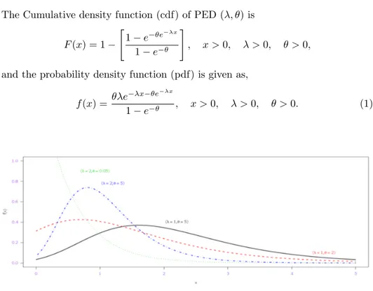
Figure 1 – The pdf plot of PED for different combinations of λ and θ.
The parameters λ and θ are the scale and shape parameters respectively of the distribution. Figure 1 shows pdfs of PED for different values of θ and λ. Its pdf is
decreasing if 0 < θ < 1 and unimodal for θ≥ 1. The modal value λe−1 is obtained at x = 1λlog(λθ).
A general expression for the rth raw moment can be given as
µ′r = E⌈Xr⌉ = ∫ xrf (x)dx (2) = ∫ xrθλe −λx−θe−λx 1− e−θ dx. (3)
The above expression can not be solved in usual form; however it can be represented in the form of special function. Following [13], it can be expressed as follows:
µ′r= θΓ(r + 1)
λr⌈1 − e−θ⌉Fr+1,r+1(⌈1, · · · , 1⌉ , ⌈2, · · · , 2⌉ , −θ) , (4)
where, Fp,q(a, b, θ) is the generalized hypergeometric function defined below:
Fp,q(a, b, θ) = ∞ ∑ j=0 ⌈ θj∏p
i=1Γ(ai+ j)Γ(ai)−1
⌉
⌈Γ(j + 1)∏q
i=1Γ(bi+ j)Γ(bi)−1⌉
, (5)
where, a =⌈a1,· · · , ap⌉; p is the number of terms of a and b = ⌈b1,· · · , bq⌉; q is
the terms of b. The proof of the Equation (4) is obtained by direct integration; see Louzada-Neto et al. [13]. It can also be noted from Louzada-Neto et al. [13] that the mean and variance of the distribution can be obtained as
E⌈X⌉ = θ λ⌈1 − e−θ⌉F2,2(⌈1, 1⌉ , ⌈2, 2⌉ , −θ) and V ar⌈X⌉ = θ λ2⌈1 − e−θ⌉[F3,3(⌈1, 1, 1⌉ , ⌈2, 2, 2⌉ , −θ) −⌈1 − eθ−θ⌉F2,2(⌈1, 1⌉ , ⌈2, 2⌉ , −θ) 2 ]
respectively. It is interesting to note here that the skewness and kurtosis are independent of scale parameter λ and depend on shape parameter θ. It is observed that skewness and kurtosis both are decreasing function of the shape parameter
θ; see Tomazella et al. [33].
2.1. Reliability characteristics
(i) Since mean does not take a very nice closed form, we shall consider here the median time to system failure (MdTSF) which is given by
M dT SF = log(θ− log(−log(0.5 + 0.5e
−θ)))
(ii) The corresponding reliability function is given by R(x) = [ 1− e−θe−λx 1− e−θ ] , x > 0, λ > 0, θ > 0.
(iii) The associated hazard function can easily be obtained as
h(x) = θλe
−λx−θe−λx
1− e−θe−λx , x > 0, λ > 0, θ > 0.
It may be noted that the initial and long term failure values are finite and are given as h(0) = lim x→0 λθe−θx (1− e−θ) = λθ (eθ− 1) and h(∞) = lim x→∞ θλe−λx eθe−λx− 1 = limx→∞ θλ θ + θ2e−λx+· · · = λ respectively.
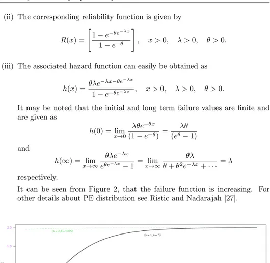
It can be seen from Figure 2, that the failure function is increasing. For other details about PE distribution see Ristic and Nadarajah [27].
Figure 2 – The failure rate plot of PED for different combinations of λ and θ.
2.2. Data collection
Let us suppose that n items, the life time of which follow PED, are put on life test. Further assume that R1items after first failure X1:m:nand R2items after failure
X2:m:n,· · · , Rm items after mth failure Xm:m:n are randomly removed from the
test. Let the sample obtained in this way is denoted by (X1:m:n, R1), (X2:m:n, R2), (X3:m:n, R3),· · · , (Xm:m:n, Rm). Where X1:m:n< X2:m:n< X3:m:n,· · · < Xm:m:n.
It may be noted here that the number of items removed at ithstage, R
iis random
of removals, say R1= r1, R2= r2, R3= r3,· · · , Rm= rm, are assumed to be fixed,
the conditional likelihood function can be written as (see Cohen [10], Kamps and Cramer [17], Balakrishnan et al. [5]):
L(α, θ; x|R = r) = f(X1:m:n,··· ,Xm:m:n)(x1,· · · , xm) = c m ∏ i=1 f (xi) [1− F (xi)] ri , −∞ < x1<· · · < xm<∞, (6) Where n = m +∑mi=1ri, n, m∈ N, ri∈ N0, 1≤ i ≤ m, ri∼ B(n−m− ∑i−1 l=0rl, p)
for i = 1, 2, 3,· · · m − 1 and r0 = 0 and c = ∏m
i=1γi with γi =
∑m
j=i(rj+ 1) and
for γ1= n.
Substituting (1) and (3.1) into (3.1), we get
L(α, λ; x|R = r) = c
m
∏
i=1
θλe−λxi−θe−λxi
1− e−θ { 1− e−θe−λxi 1− e−θ }ri . (7)
As mentioned earlier also, the number of items removed are random and inde-pendent of each other with probability p for each unit at every stage. Thus, the number of the units Ri removed at ithfailure Xi:m:n; i = 1, 2,· · · (m − 1), follows
a binomial distribution with parameters ( n− m −∑il=1−1ri, p ) . Therefore, P (R1= r1; p) = ( n− m r1 ) pr1(1− p)n−m−r1, (8) and for i = 2, 3,· · · , m − 1, P (Ri; p) = P (Ri= ri|Ri−1= ri−1,· · · R1= r1) = ( n− m −∑il=0−1rl ri ) pri(1− p)n−m− ∑i−1 l=0rl. (9)
We further assume that Ris are independent of Xi:m:nfor all i. Then full likelihood
function takes the following form
L (θ, λ, p; x) = L (θ, λ; x|R = r) P (R = r; p) , (10)
where
P (R = r; p) = P (R1= r1) P (R2= r2|R1= r1) P (R3= r3|R2= r2, R1= r1)
· · · P (Rm−1= rm−1|Rm−2= rm−2,· · · R1= r1) .
(11) Substituting (8) and (9) into (11), we get
P (R = r; p) = (n− m)!p ∑m−1 i=1 ri(1− p)(m−1)(n−m)− ∑m−1 i=1 (m−i)ri ( n− m −∑il=1−1ri ) !∏mi=1−1ri! . (12)
Now, using (7),(10) and (12), we can write the full likelihood function in the following form L (λ, θ, p; x) = AL1(λ, θ) L2(p) , (13) where A = c(n−m)! (n−m−∑i−1l=1ri)!∏m−1i=1 ri!, L1(θ; λ) = m ∏ i=1
θλe−λxi−θe−λxi
1− e−θ { 1− e−θe−λxi 1− e−θ }ri , (14) and L2(p) = p ∑m−1 i=1 ri(1− p)(m−1)(n−m)− ∑m−1 i=1 (m−i)ri. (15)
3. Parameter estimation of λ, θ and reliability characteristics For this PED(λ, θ) we use two known methods for estimating the parameter λ and
θ, namely ML method and LS method. It is noted that the estimate can not be
expresses in nice closed form when both of the parameters are unknown in either two methods.
3.1. Maximum likelihood estimators
In this section, we have obtained the MLEs of the parameters λ, θ and p based on PT-II CBRs. We observe from (13), (14) and (15) that likelihood function is multiplication of three terms, namely, A, L1 and L2. Out of these A does not dependent on the parameters θ, λ and p, thus, it behaves as constant for given data set. L1 does not involved p and can be treated as function of θ and λ only, where as L2 involves p only. Therefore, the MLEs of θ and λ can be derived by maximizing L1. Similarly the MLE of p can be obtained by maximizing L2. Taking log of both sides of (14), we have
ln L1(λ; θ) = m ln (λ) + m ln (θ)− λ m ∑ i=1 xi− θ m ∑ i=1 e−λxi + m ∑ i=1 riln(1− e−θe −λxi )− n ln(1 − e−θ). (16)
The normal equations can be obtained by differentiating (16) with respect to
θ and λ and equating these to zero. Thus, MLEs of θ and λ can be obtained by
simultaneously solving the following normal equations :
m θ − m ∑ i=1 e−λxi+ m ∑ i=1 rie−λxi−θe −λxi 1− e−θe−λxi − ne−θ 1− e−θ = 0 (17)
and m λ − m ∑ i=1 xi+ θ m ∑ i=1 xie−λxi− θ m ∑ i=1 rixie−λxi−θe −λxi 1− e−θe−λxi = 0. (18)
It may be noted that (17) and (18) can not be solved simultaneously to provide a nice closed form for the estimators. Therefore, we propose the use of fixed point iteration method for solving these equations. For further details see Jain et al. [15], Rao [28] and Singh et al. [30]. Hence, the MLEs of MdTSF, R(t) and h(t) can be evaluated using invariance property of MLEs as
ˆ
M dT SF = log(ˆθ− log(−log(0.5 + 0.5e
−ˆθ))) ˆ λ ˆ R(t) = [ 1− e−ˆθe−ˆλt 1− e−ˆθ ] , t > 0 ˆ h(t) = ˆ θˆλe−ˆλt−ˆθe−ˆλt 1− e−ˆθe−ˆλt , t > 0.
The MLE of parameter p can be obtained by maximizing (15). Thus we find immediately, ˆ pmle= ∑m−1 i=1 ri (m− 1) (n − m) −∑mi=1−1ri(m− i − 1) .
3.2. Least square estimation
In this section, we drive The least squares estimators (LSEs) of the two parameters of PED, with modifications necessary to make for PT-II CBR sample. The LSEs were originally proposed by Swain et al. [29] for Beta distribution.
Let X1:m:n, X2:m:n,· · · , Xm:m:n be a PT-II CBR sample with sample size n,
failure information m and censoring scheme with random R = (R1, R2,· · · , Rm)
from a population with cdf F (.). Then, for i = 1, 2,· · · , m see (Balakrishnan and Aggarwala [4][pp. 22-23], Balakrishnan et al. [5]).
E (F (Xi:m:n)) = 1− m ∏ j=m−i+1 αj where αj =(1+aaii) and ai= i + m ∑ j=m−i+1 rj
Now, the LSE of the parameters can be obtained by minimising
Q = m ∑ i=1 [F (Xi:m:n)− E (F (Xi:m:n))] 2 (19)
with respect to the parameters.
In the case of PED, the LSEs of (λ, θ) can be obtained by minimizing,
Q (λ, θ) = m ∑ i=1 ∏m j=m−i+1 αj− { 1− e−θe−λxi 1− e−θ } 2 (20)
with respect to the parameters λ and θ. Thus, the LSEs of (λ, θ) are the solutions of the following simultaneous equations:
∂Q (λ, θ) ∂λ = m ∑ i=1 ∏m j=m−i+1 αj− { 1− e−θe−λxi 1− e−θ } θxi { e−(θe−λxi+λxi) 1− e−θ } = 0, (21) ∂Q (λ, θ) ∂θ = m ∑ i=1 m ∏ j=m−i+1αj − 1− e−θe−λxi 1− e−θ e−θ (1− e−θe
−λxi)− (1 − e−θ )e−(θe−λxi +λxi)
(1− e−θ )2 = 0. (22)
The solutions of the simultaneous Equations (21) and (22) can be evaluated numerically by some suitable iterative procedure such as Newton-Raphson method, for given the values of (n, m, R, Xi:m:n) for i = 1, 2, 3,· · · , m.
3.3. Asymptotic confidence intervals
The first derivatives of the log likelihood of PED with respect to λ and θ are given by equation (17) and (18) and hence the second derivatives are
∂2ln L1(λ; θ) ∂θ2 =− m ∑ i=1 rie−θe −λxi−λxi{ e−λxi ( e−θe−λxi − 1 ) − e−θe−λxi} ( 1− e−θe−λxi)2 −m θ2 + n (1− e−θ)2 (23) ∂2ln L 1(λ; θ) ∂λ2 =−θ m ∑ i=1 rixie−λxi−θe −λxi{( 1− e−θe−λxi ) (θxie−λxi− xi) + ( θxie−λxi−θe −λxi)} ( 1− e−θe−λxi )2 −m λ2 − m ∑ i=1 x2ie−λxi (24) ∂2ln L 1(λ; θ) ∂λ∂θ = ∂2ln L 1(λ; θ) ∂θ∂λ = m ∑ i=1 xie−λxi+ θ m ∑ i=1 rie−λxi−θe −λxi{( 1− e−θe−λxi ) (θxie−λxi− xi) + ( θxie−λxi−θe −λxi)} ( 1− e−θe−λxi )2 (25)
If we denote the MLE of ζ = (λ, θ) by (ˆλM L, ˆθM L), the observed information matrix is then given by I(δ) = [ ∂2lnL1(λ;θ) ∂λ2 ∂2lnL1(λ;θ) ∂λ∂θ ∂2lnL1(λ;θ) ∂θ∂λ ∂2lnL1(λ;θ) ∂θ2 ] λ=ˆλM L,θ= ˆθM L (26)
And hence the variance covariance matrix would be I−1(δ). The approximate (1−α)100%
confidence intervals (CIs) for the parameters λ and θ are ˆλM L± ζα/2
√
V (ˆλM L) and
ˆ
θM L±ζα/2
√
V (ˆθM L), respectively where V (ˆλM L) and V (ˆθM L) are variances of ˆλM Land
ˆ
θM L, which are given by the first and the second, diagonal element of I−1(δ), and ζα/2
is the upper (α/2) percentile of standard normal distribution.
4. Numerical study
The estimators ˆλM L and ˆθM L denote the MLEs of the parameters λ and θ respectively
while ˆλLS and ˆθLS are corresponding LSEs. Also ((λLc λUc) and (θLc θUc)) represent
average CI. We have obtained the estimates and reliability characteristics from MLEs and estimates from LSEs. The comparisons are based on MSE through the simulated sample of estimates. It may be mentioned here that the exact expressions for the estimates can not be expressed in closed form. Therefore, the estimates are estimated on the basis of Monte-Carlo simulation study of 10000 samples. We have taken (λ = 2, θ = 5) and (λ = 2, θ = 6) for three different sample sizes (i) small sample size n = 20, (ii) moderate sample size n = 30, and (iii) large sample size n = 50. Also, each sample size has 4 censoring schemes. For the arbitrary chosen value of this parameter (λ = 2, θ = 5) has been all ready studied in bayesian paradigm under PT-II CBR by Singh et al. [32]. So, We study this values in classical frame under MLE and LSE. The study contains the following steps:
(a) Take the values of the parameters λ, θ and mission time t. (b) Compute the actual values of MdTSF, R(t) and h(t).
(c) Generate a PT-II CBR sample of size n with m failures using the algorithm given by Balakrishnan and Shandhu [3].
(d) For each value of (n = 20, 30, 50), four values of m are considered, so that, the
percentage of failure information (m/n)× 100 is 40, 50, 80 and 100%.
(e) Compute the MLEs of λ, θ, M dT SF, R(t) and h(t) according to Subsection 3.1. Also, compute CI for both λ and θ (using normal approximation) and corresponding compute LSEs of λ and θ according to Subsection 3.2.
(f) Repeat steps (c)−(d), N = 10, 000 times for chosen values of (λ = 2, θ = 5, t =
1.8, p = 0.5) and (λ = 2, θ = 6, t = 1.8, p = 0.5) with each of 12 censoring schemes. Compute the expected value (EV), mean square error (MSE) of the
es-timates obtained in step (d) using the following formulae EV = 1
N N ∑ i=1 ˆ ϕ (δ) and MSE= 1 N N ∑ i=1 ( ˆ ϕ (δ)− ϕ (δ) )2
, where δ = (λ, θ), ϕ (.) is function of the set of model
4.1. Comparison of simulation study
The simulation study was performed for various values of effective sample m for both
parameters are unknown. Briefly, we are giving here the simulation (Tables 1−3), for
both parameters are unknown with (λ = 2, θ = 5) and (λ = 2, θ = 6) under different percentage of failure information. The conclusions for these studies are given below. (a) Tables 1 shows the LSE of λ and θ and the corresponding reliability characteristics
respectively. From Tables 1, one can note that the MSE and bais decrease as the effective sample size(m) get near to n.
(b) The MLEs are presented in Tables (1-2). It is also observed similar pattern as
Tables 1.
(c) One can see, based on Tables 1 and Tables 2, the LSEs of λ, θ perform better as compare to MLE in terms of bais and MSE.
(d) In Tables 2-4, 6 and 5, 7, ((λLc λUc) and (θLc θUc)) are presented an average limit
of lower and upper limit of λ and θ respectively. It can be seen from these tables that as m increases the average length of the intervals decreases.
5. Real data analysis
In this section, we consider two types of real data example. First data set is a result of a test on endurance of deep groove ball bearings and was originally discussed by Lieblein and Zelen [21] and also given in Lawless [20]. Second data set in this example was extracted from Ed Fuller of the NICT Ceramics Division. It contains polished window strength data. A paper by Pepi [16] describes the all-glass airplane window design. Since the data were used in a case of study is a form of reliability analysis Under PT-II CBRs. The second data sets are as follows: 18.83, 20.8, 21.657, 23.03, 23.23, 24.05, 24.321, 25.5, 25.52, 25.8, 26.69, 26.77, 26.78, 27.05, 27.67, 29.9, 31.11, 33.2, 33.73, 33.76, 33.89, 34.76, 35.75, 35.91, 36.98, 37.08, 37.09, 39.58, 44.045, 45.29, 45.381. In order to have an idea about the associated failure rate for both example, we considered, a graphical method based on TTT (Total Time on Test) plot as a crude indicator see Aarset [1]. The empirical TTT is given as T (nr) = ∑r i=1∑x(i)+(n−r)x(r) n i=1x(i) ,
where r = 1, 2,· · · , n and x(r) is the order statistics of the sample. Figure (5,8) shows
the TTT plot, which is concave indicating that data relates to an increasing failure
rate. Thus, It can be properly accommodated by a PED. The fitting of PED was
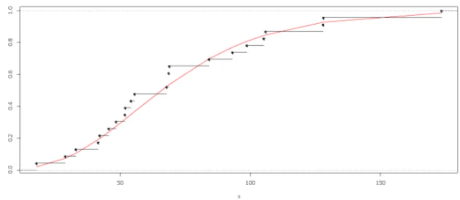
checked using CDF-plot and PP-plot given in Figure (3-4), Figure (6-7) and
Kolmogorov-Smirnov(KS) test. Value of the test statistics 0.115023 < 0.275(KS(T abulated)) and
0.1052121 < 0.2903226(KS(T abulated)), which shows that PED provides a satisfactory
fit to the considered two data sets respectively. On the basis of these data set the MLEs, LSEs, intervals of λ and θ are presented in Table 5 and Table 7 respectively. But for the purpose of illustrating the method discussed in this paper, a PT-II CBR is generated from these data sets under different schemes. The number of removals are shown in Table 4 Table 6 under different schemes. Using the formulae given in section (3) under different degree of censoring, the LSEs and MLEs of λ and θ are presented in Table 5 and Table 7 respectively.
6. Conclusion
In this paper, we have considered the problem of classical estimation of parameters of PED under PT-II CBR sample. We have found that in most of the considered method of estimations, LSEs provides the precise estimate with smaller MSE as well as bais. Finally, we may conclude that the LSEs discussed in this article can be recommended for use of PED parameter estimation under PT-II CBRs sample.
Acknowledgements
The authors wish to thank editors and executive editor, Department of Statistics, Uni-versity of Bologna (Italy) and the referee for their valuable comments without which the paper could not have taken its present form.
Appendix
T ABLE 1 The LSEs, ˆ λLS , ˆ θLS with N=10000. (λ = 2 , θ = 5) (λ = 2 ,θ = 6) ˆ λLS ˆ θLS ˆ λLS ˆ θLS n m EV MSE EV MSE EV MSE EV MSE 20 8 2.257866 0.1432075 5.217637 0.07505436 2.257793 0.1388416 6.211979 0.06751352 10 2.253057 0.1307837 5.211601 0.06776987 2.245029 0.120462 6.220359 0.07074178 16 2.210637 0.08508801 5.207937 0.06635705 2.216674 0.09082911 6.214638 0.06917726 20 2.205179 0.0815763 5.207617 0.06114342 2.210007 0.08497755 6.193346 0.05463395 30 12 2.218481 0.1220195 5.214065 0.07356288 2.236031 0.1122036 6.218901 0.07189593 15 2.244198 0.09963355 5.210096 0.06802988 2.228203 0.1016959 6.208113 0.06483563 24 2.195392 0.07115373 5.209478 0.06758128 2.19641 0.07234936 6.202962 0.06024173 30 2.189607 0.0605371 5.208539 0.06393413 2.176261 0.05928837 6.204176 0.05940488 50 20 2.206203 0.07857486 5.238891 0.09442493 2.191333 0.0670037 6.216795 0.07098946 25 2.203551 0.07345039 5.226853 0.08115761 2.184433 0.06142801 6.214154 0.06977389 40 2.159913 0.04543208 5.209465 0.06696698 2.15157 0.03682177 6.21612 0.06889521 50 2.165206 0.04367941 5.203225 0.06356012 2.140585 0.03277235 6.210628 0.06807916 Here, EV=exp ected v alue; MSE=mean square error.
T ABLE 2 The MSEs, ˆλ M L , ˆθ M L , ˆ M dT S F , ˆR M L (t ) and ˆh M L (t ) with N=10000, λ = 2 , θ = 5 , t = 1 .8 , R (t ) = 0 .12177 , h (t ) = 1 .8664 , M dT S F = 0 .9928 ˆλ M L ˆθ M L ˆR M L ( t ) and ˆh M L ( t ) ˆ M dT S F n m EV MSE λ L c λ U c EV MSE θ L c θ U c EV R M S E ( t ) EV h M S E ( t ) EV M dT S F M S E 20 8 2.516772 0.4515471 1.112505 3.921038 6.043283 1.385528 0.7784289 11.30814 0.0741134 0.003924923 2.425185 0.530386 0.3286175 0.6284103 10 2.434744 0.3225734 1.210062 3.659426 5.999493 1.325861 0.9982802 11.00071 0.08001229 0.003149592 2.336998 0.380646 0.889639 0.02626591 16 2.338223 0.1788687 1.39232 3.284126 5.968235 1.267764 1.452574 10.4839 0.08853164 0.00220595 2.231794 0.2138113 0.93350628 0.01307016 20 2.316086 0.1657632 1.46048 3.171693 5.962575 1.240088 1.63123 10.29392 0.09182791 0.002009896 2.206689 0.1975083 0.94065402 0.01050037 30 12 2.401921 0.2557954 1.313118 3.490725 6.009535 1.346643 1.706662 10.31241 0.08231192 0.002811488 2.301634 0.304476 0.90694587 0.01827684 15 2.353267 0.2055738 1.390486 3.316048 5.92027 1.167238 1.863624 9.976917 0.086872 0.002454561 2.248781 0.2458692 0.93138544 0.01318454 24 2.297906 0.1380174 1.539019 3.056793 5.963833 1.237799 2.262185 9.66548 0.0931578 0.001757219 2.187035 0.1645452 0.94887726 0.00867817 30 2.25518 0.1017315 1.577246 2.933115 5.964612 1.225471 2.438641 9.490584 0.09925675 0.001351311 2.138516 0.1207596 0.96033982 0.006650774 50 20 2.302762 0.1415643 1.502238 3.103285 5.963766 1.234209 3.079802 8.847729 0.09187583 0.00179172 2.193088 0.1688115 0.93891037 0.01026392 25 2.27523 0.1234666 1.561433 2.989027 5.955072 1.218825 2.749572 9.160572 0.09651679 0.00155424 2.161273 0.1467117 0.94556656 0.008999505 40 2.231225 0.08292604 1.662612 2.799837 5.942028 1.197306 2.594613 9.289444 0.1023322 0.001081027 2.111676 0.09759213 0.96651341 0.005665663 50 2.204684 0.0624741 1.692183 2.717186 5.893823 1.09636 3.203957 8.583689 0.1047418 0.0008482828 2.082988 0.07317595 0.97424549 0.004061965
T ABLE 3 The MSEs, ˆ λM L , ˆ θM L , ˆ M dT S F , ˆ RM L (t ) and ˆ hM L (t ) with N=10000, λ = 2 , θ = 6 , t = 1 .8 , R (t ) = 0 .1490 , h (t ) = 1 .84053 , M dT S F = 1 .080 ˆ λM L ˆ θM L ˆ RM L (t ) and ˆ hM L (t ) ˆ MdT S F n m EV MSE λL c λU c EV MSE θL c θU c EV RM S E (t ) EV hM S E (t ) EV M dT S FM S E 20 8 2.44921 0.34048 1.12241 3.77600 7.00744 1.34651 1.66921 12.34568 0.09335 0.00510 2.33702 0.41789 0.55754 0.00055 12 2.37823 0.24576 1.21768 3.53878 6.98553 1.28297 1.11919 12.85188 0.10184 0.00401 2.25743 0.30303 0.57445 0.00051 16 2.32126 0.15674 1.40911 3.23340 6.97512 1.27222 0.82919 13.12105 0.10718 0.00308 2.19465 0.19519 0.58913 0.00048 20 2.26969 0.12342 1.45618 3.08320 6.97101 1.25968 1.88605 12.05596 0.11581 0.00241 2.13520 0.15305 0.60152 0.00046 30 12 2.33507 0.19187 1.31376 3.35637 6.99414 1.32647 2.83962 11.14865 0.10704 0.00334 2.20905 0.23714 0.58540 0.00049 15 2.32770 0.17555 1.41198 3.24342 7.00376 1.32504 2.63630 11.37122 0.10718 0.00323 2.20144 0.21792 0.58700 0.00049 24 2.25934 0.10217 1.53592 2.98276 6.99823 1.31990 1.96458 12.03187 0.11656 0.00212 2.12368 0.12652 0.60517 0.00045 30 2.22374 0.07862 1.57600 2.87148 6.98875 1.31094 2.19541 11.78209 0.12268 0.00165 2.08244 0.09669 0.61459 0.00043 50 20 2.29358 0.13113 1.52637 3.06079 6.98082 1.29346 3.05647 10.90517 0.11079 0.00262 2.16347 0.16298 0.59552 0.00047 25 2.25073 0.09316 1.56827 2.93320 6.95276 1.20540 3.21393 10.69159 0.11689 0.00202 2.11487 0.11575 0.60609 0.00045 40 2.20912 0.06619 1.66167 2.75657 6.92932 1.18913 3.75441 10.10423 0.12355 0.00145 2.06723 0.08152 0.61653 0.00043 50 2.18611 0.05159 1.69380 2.67843 6.91783 1.16204 3.56315 10.27250 0.12772 0.00109 2.04033 0.06259 0.62334 0.00042
T ABLE 4 PT-II CBR samples under differ ent censoring scheme (S n :m ) for fixe d n = 23, p = 0 .5 Sc heme i 1 2 3 4 5 6 7 8 9 10 11 12 S 23:9 r i:9:23 2 2 2 0 0 2 2 2 2 x i:9:23 17.88 41.52 48.4 54.12 55.56 67.8 68.88 98.64 127.92 S 23:9 r i:9:23 0 0 0 0 0 0 0 0 14 x i:9:23 17.88 28.92 33 41.52 42.12 45.6 48.4 51.84 51.96 S 23:12 r i:12:23 1 1 1 1 1 0 0 0 0 2 2 2 x i:12:23 98.64 127.92 17.88 33 42.12 48.4 51.96 55.56 67.8 68.64 68.64 68.88 S 23:12 r i:12:23 0 0 0 0 0 0 0 0 0 0 0 11 x i:12:23 17.88 28.92 33 41.52 42.12 45.6 48.4 51.84 51.96 54.12 55.56 67.8 S 23:18 r i:18:23 1 1 0 0 0 0 0 0 0 0 0 0 x i:18:23 17.88 33 42.12 45.6 48.4 51.84 51.96 54.12 55.56 67.8 68.64 68.64 S 23:18 r i:18:23 0 0 0 0 0 0 0 0 0 0 0 0 x i:18:23 17.88 28.92 33 41.52 42.12 45.6 48.4 51.84 51.96 54.12 55.56 67.8 0 0 0 1 1 1 68.88 84.12 93.12 98.64 105.84 128.04 0 0 0 0 0 5 68.64 68.64 68.88 84.12 93.12 98.64
T ABLE 5 The LSEs, ˆ λLS , ˆ θLS and MLEs ˆ λM L , ˆ θM L , ˆ MdT S F , ˆ R(t ), ˆ h(t ) and 95% confidenc e intervals (CI) for λ and θ with various censoring schemes. Sc heme 95%CI of λ 95%CI of θ t=72.22 Sm :n ˆ λLS ˆ λM L λL c λU c ˆ θLS ˆ θM L θL c θU c ˆ M dT S FM L ˆ R(t )M L ˆ h(t )M L S9:23 0.0311 0.0206 0.0084 0.0328 8.3512 5.0000 0.6139 9.3862 96.5497 0.1540 0.0497 S9:23 0.0356 0.0448 0.0229 0.0667 7.0001 10.1288 0.6727 19.5849 59.8729 0.4150 0.0269 S12:23 0.0378 0.0239 0.0117 0.0361 7.0044 5.0000 0.8872 9.1128 83.1250 0.3667 0.0298 S12:23 0.0341 0.0376 0.0207 0.0546 7.0001 7.9278 1.3387 14.5168 64.7733 0.4481 0.0250 S18:23 0.0384 0.0345 0.0219 0.0472 7.0000 7.8575 2.0622 13.6527 70.3525 0.3530 0.0307 S18:23 0.0356 0.0359 0.0224 0.0493 6.9995 7.3285 1.9028 12.7542 65.7969 0.4150 0.0269 S23:23 0.0374 0.0358 0.0237 0.0480 6.9929 7.3241 2.2388 12.4094 65.8346 0.3750 0.0292
T ABLE 6 PT-II CBR samples under differ ent censoring scheme (S n :m ) for fixe d n = 31, p = 0 .5 Sc heme i 1 2 3 4 5 6 7 8 9 10 11 12 13 S 31:9 r i :9:31 2 2 4 4 4 4 0 0 2 x i :9:31 18.83 23.03 24.321 26.77 31.11 34.76 37.09 39.58 44.045 S 31:9 r i :9:31 0 0 0 0 0 0 0 0 23 x i :9:31 18.83 20.8 21.657 23.03 23.23 24.05 24.321 25.5 25.52 S 31:12 r i :12:31 1 1 1 1 1 0 0 1 1 4 4 4 x i :12:31 18.83 21.657 23.23 24.321 25.52 26.69 26.77 26.78 27.67 31.11 34.76 37.09 S 31:12 r i :12:31 0 0 0 0 0 0 0 0 0 0 0 19 x i :12:31 18.83 20.8 21.657 23.03 23.23 24.05 24.321 25.5 25.52 25.8 26.69 26.77 S 31:18 r i :18:31 1 0 0 0 0 0 0 0 0 0 0 0 0 x i :18:31 18.83 21.657 23.03 23.23 24.05 24.321 25.5 25.52 25.8 26.69 26.77 26.78 27.05 0 0 4 4 4 27.67 29.9 31.11 34.76 37.09 S 31:18 r i :18:31 0 0 0 0 0 0 0 0 0 0 0 0 0 x i :18:31 18.83 20.8 21.657 23.03 23.23 24.05 24.321 25.5 25.52 25.8 26.69 26.77 26.78 0 0 0 0 13 27.05 27.67 29.9 31.11 33.2 S 31:18 r i :18:31 0 0 0 0 0 0 0 0 0 0 0 0 0 x i :18:31 18.83 20.8 21.657 23.03 23.23 24.05 24.321 25.5 25.52 25.8 26.69 26.77 26.78 0 0 0 0 0 0 0 0 0 0 0 0 0 27.05 27.67 29.9 31.11 33.2 33.73 33.76 33.89 34.76 35.75 35.91 36.98 37.08 0 0 0 0 0 37.09 39.58 44.045 45.29 45.381
T ABLE 7 The LSEs, ˆ λLS , ˆ θLS and MLEs ˆ λM L , ˆ θM L , ˆ MdT S F , ˆ R(t ), ˆ h(t ) and 95% confidenc e intervals (CI) for λ and θ with various censoring schemes. Sc heme 95%CI of λ 95%CI of θ t=30 Sm :n ˆ λLS ˆ λM L λL c λU c ˆ θLS ˆ θM L θL c θU c ˆ M dT S FM L ˆ R(t )M L ˆ h(t )M L S9:31 0.09994 0.08981 0.04760 0.13202 20.00000 24.03873 0.00120 52.93034 39.48511 0.60140 0.06093 S9:31 0.10238 0.19047 0.09493 0.28602 20.00000 23.05342 0.00320 53.75884 28.74743 0.57391 0.06485 S12:31 0.10236 0.10973 0.06178 0.15769 21.40992 31.14815 0.00450 71.28121 34.67729 0.59908 0.06261 S12:31 0.09811 0.19632 0.11248 0.28016 19.91707 49.00043 0.00560 59.30896 28.49229 0.62059 0.05813 S18:31 0.12844 0.13788 0.08712 0.18863 32.50901 51.60121 0.00100 68.15195 31.26041 0.46279 0.09264 S18:31 0.11494 0.14517 0.09183 0.19852 22.56790 57.50334 0.00030 76.05151 30.43498 0.47997 0.08143 S31:31 0.12666 0.16703 0.12067 0.21339 19.99992 97.19058 0.00018 103.04340 29.59390 0.33226 0.10280
Figure 4 – PP plot for endurance of deep groove ball bearings data.
Figure 5 – TTT plot for endurance of deep groove ball bearings data.
Figure 7 – PP plot for glass airplane window data.
References
1. M. V. Aarset (1987). How to identify bathtub hazard rate. IEEE Transactions and Reliability, R-36, 106–108.
2. K. Adamidis, S. Loukas (1998). A lifetime distribution with decreasing failure rate. Statistics and Probability Letters, 39(1), 35–42.
3. N. Balakrishnan, R. A. Sandhu (1995). A simple simulational algorithm for generating progressive Type-II censored samples.American Statistics, 49(2), 229– 230.
4. N. Balakrishnan, R. Aggarwala (2000). Progressive Censoring: Theory, Meth-ods, and Applications. Birkhauser, Boston.
5. N. Balakrishnan, E. Cramer, U. Kamps (2001). Bounds for means and vari-ances of progressive Type-II censored order statistics. Statistics and Probability Letters, 54, 301–315.
6. N. Balakrishnan, N. Kannan (2001). Point and Interval Estimation for Param-eters of the Logistic Distribution Based on Progressively Type-II Censored Samples. In N. Balakrishnan, C. R. Rao Handbook of Statistics , 20, Eds. Amsterdam, North-Holand.
7. N. Balakrishnan (2007). Progressive censoring methodology: an appraisal (with Discussions). Test, 16, 211–296.
8. W. Barreto-Souza, F. A. Cribari-Neto (2009). Generalization of the exponential-poisson distribution. Statistics and Probability Letters, 79, 2493–2500.
9. A. Basu, L. Klein (1982). Some Recent Development in Competing Risks Theory. Survival Analysis, IMS, Hayward, 1.
10. A. C. Cohen (1963). Progressively censored samples in life testing.. Technomet-rics, 327–339.
11. A. Childs, N. Balakrishnan (2000). Conditional inference procedures for the laplace distribution when the observed samples are progressively censored. Metrika, 52, 253–265.
12. E. Cramer, G. Iliopoulos (2010). Adaptive progressive Type-II censoring. Test, 19, 342–358.
13. V G. Cancho, F. Louzada-Neto, G. D. C. Barriga (2011). The poisson-exponential lifetime distribution. Computational Statistics and Data Analysis, 55, 677–686.
14. R. D. Gupta, D. Kundu (1999). Generalized exponential distribution. Australian and New Zealand Journal of Statistics, 41(2), 173-188.
15. M. K. Jain, S. R. K. Iyengar, R. K. Jain (1984). Numerical Methods for Scientific and Engineering Computation. New Age International (P) Limited, New Delhi, fifth edition.
16. J. W. Pepi (1994). Failsafe design of an all BK-7 glass aircraft window.. SPIE Proc, 2286, 431–443.
17. U. Kamps, E. Cramer (2001). On distributions of generalized order statistics. Statistics, 35, 269–280.
18. K. Krishna, K. Kumar (2012). Reliability estimation in generalized inverted ex-ponential distribution with progressively type II censored sample.Journal Statistical Computation and Simulation, 1, 1–13.
19. C. Kus (2007). A new lifetime distributions. Computational Statistics and Data analysis, 11, 4497–4509.
20. J. F. Lawless (1982). Statistical Models and Methods for Lifetime Data. Wiley, NewYork.
21. J. Lieblein, M. Zelen (1956). Statistical investigation of the fatigue life of deep groove ball bearings. J. Res. Nat. Bur. Stand., 57, 273–316.
22. F. Louzada-Neto (1999a). Modelling life time data: A graphical approch. Appl. Stochastic. Models Bus. Ind., 15, 123–129.
23. F. Louzada-Neto (1999b). Poly-hazard regression models for lifetime data. Bio-metrics,55, 1121–1125.
24. F. Louzada-Neto, V. G. Cancho, G D. C. Barriga (2011). The Poisson-exponential distribution: a Bayesian approach. Journal of Applied Statistics, 38(6), 1239–1248.
25. M. Mousa, Z. Jaheen ((2002)). Statistical inference for the Burr model based on progressively censored data. An International Computers and Mathematics with Applications, 43, 1441–1449.
26. H. K. T. Ng, P. S. Chan, N. Balakrishnan (2002). Estimation of parameters from progressively censored data using an algorithm. Computational Statistics and Data Analysis, 39, 371–386.
27. M. M. Ristic, S. Nadarajah (2010). A new lifetime distribution. Research Re-port No. 21. Probability and Statistics Group School of Mathematics, University of Manchester, Manchester.
28. G. Shanker Rao (2006). Numerical Analysis. New Age International (P) Ltd. 29. J. Swain, S. Venkatraman, J. Wilson (1988). Least squares estimation of
distribution function in Johnson’s translation system. J. Statist. Comput. Simul., 29(4), 271–297.
30. S. K. Singh, U. Singh, M. Kumar (2013). Estimation of parameters of general-ized Inverted exponential distribution for progressive Type-II Censored Sample with Binomial Removals.Journal of Probability and Statistics, 1–12.
31. S. K. Singh, U. Singh, M. Kumar (2014). Estimation for the Parameter of Poisson-Exponential distribution under Bayesian Paradigm. Journal of Data Sci-ence, 12, 157–173.
32. S. K. Singh, U. Singh, M. Kumar (2014). Bayesian estimation for Poisson-exponential model under Progressive type-II censoring data with binomial removal and its application to ovarian cancer data. Communications in Statistics - Simu-lation and Computation, DOI:10.1080/03610918.2014.948189, accepted.
33. V. L. D. Tomazella, V. G. Cancho, F. Louzada (2013). The bayesian refer-ence analysis for the poisson-exponential lifetime distribution. Chilean Journal of Statistics, 4(1), 99–113.
34. S. K. Tse, C. Yang, H. K. Yuen (2000). Statistical analysis of Weibull dis-tributed life time data under type II progressive censoring with binomial removals. Jounal of Applied Statistics, 27, 1033–1043.
35. S. J. Wu, C. T. Chang (2002). Parameter estimations based on exponential progressive type II censored with binomial removals. International Journal of In-formation and Management Sciences, 13, 37–46.
36. S. J. Wu, C. T. Chang (2003). Inference in the Pareto distribution based on progressive Type II censoring with random removals. Journal of Applied Statistics, 30(2), 163–172.
37. H. K. Yuen, S. K. Tse (1996). Parameters estimation for Weibull distributed lifetimes under progressive censoring with random removeals. Journal Statistical Computation and Simulation, 55 (1-2), 57–71.
Summary
In this paper, a poissoin-exponential distribution(PED) is considered as a lifetime model. Its statistical characteristics and important distributional properties are discussed by Louzada-Neto et al. [13]. The method of Maximum likelihood estimation and least square estimation of parameters involved along with reliability and failure rate functions is also studied here. In view of cost and time constraints, Progressive type-II censored data with binomial removals (PT-II CBRs) have been used. Finally, two real data examples are given to show the practical applications of the paper.