RECENT PROPOSAL FOR THE ESTIMATION OF HOUSEHOLD HUMAN CAPITAL
G. Vittadini, P.G. Lovaglio
1. INTRODUCTION
The concept of Human Capital (HC), formally introduced and quantified by Petty (1690) and Cantillon (1755) and conceptually analyzed by Adams Smith (1776) was further discussed by distinguished economists throughout history such as Pareto, Marshall, Irving Fisher and C. Gini. In the second half of the 20th
century, the study of HC acquired a renewed interest. In this period, several economists concentrated on the qualitative analysis of HC, abandoning the quan-titative estimation of personal HC and opting for the earning function as a func-tion of years of schooling alone (Mincer, 1958; 1970) or as a funcfunc-tion of years of schooling, professional investment in HC and on the job training (Becker, 1962; 1964). Other economists, conscious of the need and the relevance of having quantitative HC estimations, followed the approach of the Retrospective Method (Kendrick, 1976; Eisner 1985). It deals with the cost of production in the tradi-tion of Cantillon (1755) and Engel (1883). The Prospective Method (Jorgenson and Fraumeni, 1989) instead follows the pioneering actuarial contribution of Wil-liam Farr (1853) and can be defined as the present actuarial value of an individ-ual’s expected income related to his skill, acquired abilities, and education (Da-gum and Slottje, 2000). The Educational Attainment method (Barro, 1991; Mankiw et al., 1992; OECD, 1998; Mulligan and Sala-I-Martin, 2000; Wö mann 2003) relates the aggregate stock of HC to the highest level of education com-pleted by each adult (OECD, 1998; Le et al., 2003; Wö mann, 2003).
2. CAMILO DAGUM’S CONTRIBUTION TO HUMAN CAPITAL
The work of Camilo Dagum has provided many important solutions to the problem of HC estimation. Dagum’s (1994) first major contribution was to pur-port a recursive model in order to explain the levels and distribution of personal HC, income and wealth and their distribution, and to interpret the causal impact of the estimated matrices upon the explained endogenous variables, by means of the estimated shor-term and long-term multiplyers.
Table 2 demonstrates explanatory (exogenous and lagged endogenous) and en-dogenous variables of the recursive model consisting of 17 independent equa-tions. The last equation in Dagum’s recursive model is the income generating function (Dagum, 1994) y= (HC*, w) which determines the level and distribution of in-come y as a function of estimated HC (HC*) and total wealth w. It can be ex-pressed in an analytical way as:
log[g1(y)]=!1+!2log[g2(HC*)]+!3log[g3(w)]+u (1)
where y, HC*, w are the n-dimensional vectors of Household income, estimated HC, and wealth, respectively and u the error in equation. The non linear relation-ship (1), both in variables and in parameters,1 becomes linear by means of a
loga-rithmic transformation. It plays a central role in linking the functional to the per-sonal distribution of income, which was, for over a century, an unsolved issue in economics. Furthermore, it offers a sound base to substantiate the micro-macro foundations of income distribution.
Secondly, after having proposed the recursive model, Dagum improved the es-timation method of HC, demonstrating that previous approaches (Prospective, Retrospective, Educational Attainment) proposed for estimating HC are not completely satisfactory.
The Prospective Method reduces HC investment to its monetary value in terms of assumed and unsubstantiated flow of income. Among other shortcom-ings, it ignores the amount of investment in education, job training and other in-vestments (Dagum and Slottje, 2000).
The Retrospective Method is insufficient for various reasons, not taking into account social costs, such as public investment in education, the variables con-cerning home conditions and community environments, and the genetic contri-bution to HC, including health conditions (Dagum and Slottje, 2000; Le et al., 2003). Moreover, the actual effects of the investment in HC on the income and wealth of the household heads are not considered.
The Educational Attainment Method does not take into account the fact that the impact of one year of schooling on the quantity and quality of the stock of HC can be strongly influenced by several aspects, such as the quality of the edu-cational system, the diverse returns of different levels of schooling, as well as per-sonal characteristics such as intelligence and family background (OECD, 1998; Le et al., 2003; Wö mann, 2003).
Of the various limitations these methods present, the principal defect common to all of them is that they provide only an aggregate measure of the HC stock. Therefore, what is needed is a new method of HC estimation, which provides a microeconomic estimation of personal and household HC distribution as
rec-ommended in the 1998 OECD report on HC (OECD, 1998 p. 89)2.
1 The g(.) are analytical functions of scale and location parameters obtained by fitting empirical
distributions to proper Dagum distribution models.
2 HC is defined as: “the knowledge, skill, competencies and attributes embodied in individuals
In order to overcome these problems, Dagum, together with other authors, (Dagum and Vittadini, 1996; Dagum and Slottje, 2000) defined personal HC as the present value of a flow of earned income, throughout an individual life span, generated by his/her ability, home and social environments, and investments in education, that is, the set of working attributes of a person for generating a steady flow of income. This definition takes into account all the methodologies: the Ret-rospective, PRet-rospective, and Educational Attainment proposals.
Statistically consistent with this point of view, Dagum and Slottje (2000) define HC as a non-observable variable, strictly speaking a latent variable. Therefore, in order to obtain its monetary estimation as a Latent Variable (LV), they utilized an exponential transformation with an actuarial mathematical approach, the Partial Least Squares Method (from here on referred to as PLS), initially purported by H. Wold (1982). PLS defines and estimates the LV HC “by deliberate approximation as a linear aggregate of its observed indicators” (Wold, 1982), the p formative in-dicators F0, connected with the investment in HC in the retrospective and
educa-tional attainment methods. We have:
HCPLS=F0gPLS (2)
where the p-dimensional vector of parameters gPLS is obtained by means of simple
iterative regressions of each observed indicator f0j on previous estimates of the
LV HC (PLS mode B) and the linear combination HCPLS is equivalent to the first
standardized principal component of p formative indicators F0.
Dagum and Slottje (2000) transformed the estimated standardized LV HCPLS
into an accounting monetary value by application of the following transforma-tion:
HC°(i)=exp[HCPLS (i)] (3)
with a mean value of:
µ(HC°)= n
i=1
HC°(i)f(i)/ n
i=1
f(i) (4)
where f(i) is the number of households in the entire population which the i-th sampled household represents; HC°(i) is the accounting monetary value of HCPLS
and n is the sample size. Utilizing an actuarial approach, the authors estimate the real monetary HC upon the idea that the expected mean income at age x+t of a person of age x should be equal to the average earned income of individuals be-ing at the present x+t years old, increased by the average productivity rate rx+j;
therefore, h(x) of the households of age x is the average expected earned income by age of the household heads actualised at a given discount rate, capitalized by
“a complex, multi-faceted concept with various intangible dimensions which are not directly ob-servable and which cannot be measured with precision by a single attribute, a set of attributes, or their combined sum.” (Le et al., 2003)
the average rate of productivity rx and weighted by the survival probability. Hence, h(x) of the household heads age x is:
, 1 1 ( ) (1 ) (1 ) t x t x x t x x t x j t j h x y y p i r !" " # # # $ $ $ # #
%
# x>x0 (5)where ! – x is the age at which the earned income flow stops, x0 is the starting
age for the estimation of the expected flow of income, yx+t is the average (real)
income of the household heads of age x+t, px,x+t is the probability of survival at
age x+t of a person of age x, i is the discount rate and r is the rate of productivity. Therefore, the estimation of the monetary HC of the population of families in monetary units is the weighted average of h(x):
µ[h(x)]= 0 -x x x ! $ h(x)f(x)/ 0 -x x x ! $ f(x) (6)
Multiplying HC°(i) by the ratio between its mean values µ(HC°) and µ(h) given in (3) and (5), respectively, the vector HC$(i), of the sample observations in
na-tional monetary units, with real mean and variance becomes:
HC$(i)=HC°(i)[µ(h(x)]/µ(HC°) i=1,2,...,n (7)
Dagum and Slottje (2000) utilize such methodology for the estimation of the 1983 American Household HC. The formative indicators proposed for HC esti-mation are shown in Table 1:
TABLE 1
Formative indicators for HC estimation (Dagum and Slottje, 2000) x1 = Age of H x2 = Region x3 = Marital Status of H x4 = Gender of S x5 = Years of Schooling of H x6 = Years of Schooling of S x7 = Number of Children
x8 = Years of Full-Time Work of H
x9 = Years of Full-Time Work of S
x11 = Household Total Wealth
x12 = Household Total Debts
3. RECENT IMPROVEMENTS IN THE HC ESTIMATION METHOD
In (2) HC estimated by means of PLS method only considers its formative in-dicators F0 equivalent to the old retrospective economic definition which does
not take into account the return of the investment in HC measured by the reflec-tive indicator income y0. In this direction, Vittadini and Lovaglio (2007), in line
with Dagum and Slottje’s aforementioned definition of HC (2000), while also tak-ing into account the definitions of latent variables proposed by Wold (1982) and
Bentler (1992),3 suggest that from the statistical point of view, HC can be defined
as a multidimensional non observable construct of formative indicators F0 and,
simultaneously as a multidimensional latent cause of the reflective indicator y0
which measures its effects. As a result we have:4
HC=F0g g&F0&F0g=1; (8)
y0=HCb+v; E(v)=0; E(vv&)=" (9)
where HC is a zerodimensional latent variable, F0 is a (n,p) matrix of centered
formative indicators, g is a (p,1) vector parameter which expresses the effects of the formative indicators F0 on HC; y0 is the (n,1) of the net earned income, b is a
scalar which expresses the effect of HC on earned income y0, v is the
n-dimensional of the errors of equations with the variance-covariance ".
TABLE 2
Exogenous and endogenous variables in the recursive Dagum model a) Exogenous variables
x1 = Age of the Household Head (H)
x2 = Gender of H
x3 = Race of H
x4 = Marital Status of H
x5 = Age of the Spouse (S)
x6 = Gender of S
b) Endogenous variables
y1 = Years of Schooling of H
y2 = Years of Schooling of S
y3 = Number of Children
y4 = Years of Full-Time Work of H
y5 = Years of not Full-Time Work of H
y6 = Years of Full-Time Work of S
y7 = Years of Not Full-Time Work of S
y8 = Job Status of H y9 = Occupation of H y10 = Industry of H y11 = Job Status of S y12 = Occupation of S y13 = Industry of S
w = Household Total Wealth
d = Household Total Debt
HC = Household Human Capital (estimated latent variable)
y = Household Income
Therefore the unobservable multidimensional construct HC is approximated by the linear combination of its formative indicators F0 which better fits the only
reflective indicator y0.
Hence, substituting equation (8) into equation (9), we have:
y0=F0gb+v=F0d+v (10)
3 Bentler (1992) says that a LV is as a multidimensional construct which causes, and therefore is
indirectly measured by means of observed indicators.
4 In the measurement model of HC the error term is not specified because it is empirically
Initially we estimate d by means of Generalized Least Squares (GLS) by re-gressing Ty0=y on TF0=F with T known matrix which contains corrections for
non sfericity of errors.5 The estimated parameters d* of d=gb are the effects of the
formative indicators F on earned income y. In fact:
d*=SF-1F&y (11)
where SF=F&"F is the variance-covariance matrix of F. Premultiplying (11) for F we obtain:
Fd*=F SF-1F&y=PFy (12)
where the (n,n) matrix PF=F(F&F)-1F& is a projector on the space spanned by F.
Given the restriction that Var(HC)=1, we obtain:
var(Fd*)=var(Fgb)=b2 var(Fg)=b2 var(HC)=b2 (13)
From (12) and (13) we obtain b*, the effect of HC on earned income y:
b*=[y&PF y]½ (14)
Therefore, from (11) and (14) we obtain the parameters g*: g*=d*/b*=[y&PFy]-1/2S
F-1F&y (15)
and the estimation of HC scores:
HC*=Fg*=TF0g* (16)
The model can be extended with more (q) reflective indicators measuring the effects of the LV HC. In that case, naming the original (non transformed) indica-tors as columns in the (n,q) matrix Y° and F° without loosing generality with Y and F, model (10) becomes:
Y=HC b&+V=Fgb&+V Vec(V)'(0, In( )) (17)
where Vec stacks the columns of V.
The solution of eq. (17) can be obtained by the Redundancy Analysis Model (van den Wollenberg, 1977), which maximizes the sum of squared correlations (cor) between each reflective variable (yj) and Fg (Redundancy index):
*jcor2(Fg,yj) j=1,...,q (18)
with respect to g, under the restriction of the HC variance unit for the Fg combination:
5 Usually the errors are strongly heteroskedastic due to the weights of each sampled household
g&F&Fg=1. (19) The estimate of HC coincides with the first redundancy component of the formative indicators F with respect to the reflective indicators Y or can be obtained within a more general framework, even in presence of concomitant indicators (Lovaglio, 2007).
It has been established that by using Lagrangian multipliers the maximization (17) under (18) is achieved with the largest " eigenvalue and corresponding g* ei-genvector of the matrix F#&Y"-1Y&F# with F# matrix obtained by Gram-Schmidt
orthogonalization on F and "* an estimation of ", obtained by means of a SURE approach (Johnston, 1984) or covariance structure methods (Lovaglio, 2004).
It should be noted that several indicators of HC, such as region, gender, and marital status are categorical, and hence the formative indicators in F are of mixed type. To deal with this situation, this method can be extended to the case of formative mixed indicators. In that case, eq.(8) is expressed as follows:
HC=Fcgcbc&+Fqgqbq& (20)
where the matrix F=(Fc,Fq) of formative indicators is partitioned into matrices Fc and Fq, of qualitative and quantitative variables, respectively. The parameter vectors g and b are also partitioned into two components g=(gc,gq) and b&=(bc&, bq&), respectively.
Therefore, we look for algorithms of optimal scaling which generalize classical multivariate techniques such as principal components, multiple regression, and canonical correlation. Our preferred choice is the application of linear models in the context of ALSOS (Alternating Least Squares with Optimal Scaling) methods, which sequentially estimates the parameter vector gc and quantifies the categorical indicators fjc (contained in Fc) by means of a unique iterative algorithm which re-spects the simultaneity required, as shown in equations (8)-(11), continuing until the values of bc, gc, Fc, HC* converge (Young et al., 1976). In this way, the case of mixed indicators is extended to the case of quantitative indicators achieving the final scores of HC* by simultaneously estimating it as an unobservable multidi-mensional construct by utilising mixed formative and reflective indicators. 4. EDUCATIONAL AND JOB HUMAN CAPITAL
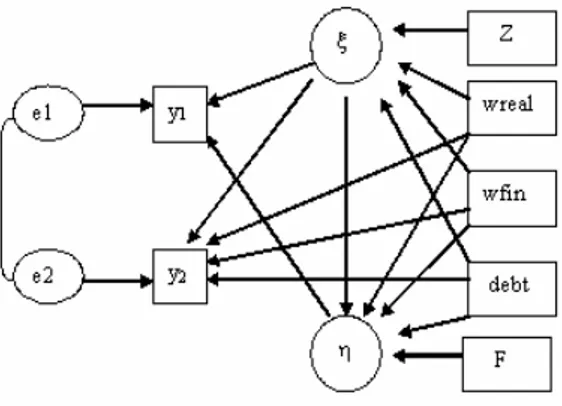
The previous approach can be extended to the case of HC of dimension two, composed of the educational dimension (EduHC, +) and working experience di-mension (JobHC, ,) underlying the process of determination of earned income and capital income, specifying a measurement model, shown in Figure 1 which is consistent with received economic theory.
The indicators which describe the force of contributing to the formation of HC (formative indicators) can be divided into four groups: indicators involving information about Household, Head (H), Spouse (S) and Parents of H and S. The
formative indicators are the Household net wealth - decomposed in three terms: real assets (wreal), financial assets (wfin), total debt (debt), and two blocks re-garding the block of educational variables (Z) and the block of (working) experi-ence indicators (F).
The life span return of HC is described by the dependent variables y1 and y2,
representing the Net disposable labour income and Net disposable capital income respectively. Once EduHC and JobHC are estimated as the best linear combina-tion (of rank one) of their formative indicators, in coherence with the supposed path (Lovaglio, 2007), we can estimate the structural model by treating the model shown in Fig. 1 as a system of three simultaneous linear equations.
Fig. 1 – Path diagram of bidimensional HC model.
5. A COMPARISON BETWEEN ITALY AND USA
First, the model is utilized for estimating the 2004 distribution of American household HC (Dagum et al., 2007).
We use the 2004 Survey of Consumer Finances (SCF) (Bucks et al., 2006), which contains detailed information regarding income, wealth and socio-demographic information on American households. The data is composed of over 4,500 households, representative of more than 110 million American fami-lies. For each household we consider indicators involving household Head (H) and Spouse (S). No adult skills or parental characteristic indicators useful for the estimation of household HC can be obtained from SCF, whereas we use house-hold earned income as the only reflective indicator.
Table 3 gives the formative indicators (and relative weights estimates) which were found significant (based on F values and significance, Sign) for determining the standardized HC.
The results confirm the expectations of economic theory, which assumes that in the process of HC formation the largest weights are found for those variables related to education and job training such as: years of schooling and job status of the head of the household, household debt, years of full time job and type of oc-cupation. Among demographic indicators, it is important to note that gender has
more weight than age and race, and within family characteristics, marital status is more important than the number of children.
TABLE 3
Formative Indicators (and statistical significance) of the HC estimation for US Families
Factors Indicators F value Sign.
Training on the Job H Job Status 4502.5 <.0001
Educational Attainment Household Debt 2590.8 <.0001
Training on the Job H Type of Occupation 1679.6 <.0001
Educational Attainment H Years of Schooling 1042.9 <.0001
Training on the Job S Job Status 1006.1 <.0001
Training on the Job H Years Full-Time Job 999.6 <.0001
Training on the Job H Sector 905.4 <.0001
Demographic H Gender 635.8 <.0001
Educational Attainment S Years of Schooling 538.3 <.0001
Demographic H Age 515.7 <.0001
Educational Attainment Educational Debt 457.6 <.0001
Demographic H Race 379.1 <.0001
Training on the Job H Part-Time Job 27.1 <.0001
Secondly, the model is utilized for estimating the 2000 distribution of Italian household HC. We use the 2000 Italian Sample Survey (Banca d’Italia, 2002) with 8,001 households, 22,268 individuals and 13,814 income-earner persons, as a rep-resentative stratified sample of 16,509 million Italian households.6 Table 4
pre-sents the most important formative indicators specified in equation (7). This equation, jointly with equation (8), estimates the standardized latent variable HC. The statistical significance of the indicators is evaluated by means of the test F (we consider indicators with F-pvalues <0.0001); in effect qqplot test reveals, for both samples, strong normality in the residuals (earned income) distribution.
The most important indicator contributing to the levels of HC is years of full time work of S which can be considered as a proxy of professional training. After this variable, in order of importance follow the variables household total wealth, years of schooling of H, years of full time work of H, and years of schooling of S. The significance of region of residence reveals the differences in HC distribution between the different regions of Italy. Moreover, on the whole, household HC is determined more by the household head than by the spouse, and even more by the years of full time job than by years of schooling.
TABLE 4
Formative Indicators (and statistical significance) of the HC estimation for Italian Families
Factors Indicators F Test Sign.
Training on the Job Years of Full-Time Work of S 472.4 <.0001
Training on the Job House Total Wealth 99.0 <.0001
Educational Attainment Years of Schooling of H 83.9 <.0001 Training on the Job Years of Full-Time Work of H 78.9 <.0001 Educational Attainment Years of Schooling of S 43.3 <.0001
Demographic Region of Residence 39.0 <.0001
Training on the Job Occupation of H 38.7 <.0001
Educational Attainment Household Total Debt 28.8 <.0001
6 The sample is representative of the household population because H and S are the 85%
Applying the actuarial method proposed by Dagum and Slottje (2000), under particular hypotheses7, we obtain the expected flow income in the cycle span for
Italian household head.
The mean, median and Gini ratio of the distributions of the household Total Wealth, Net Wealth, Income, Total Debt and the monetary estimated American and Italian household distributions of HC are presented in Table 5. The HC av-erage is more than sixteen times higher than the avav-erage income of American families and ten times higher than Italian families. Moreover, the HC average is slightly higher than the average total wealth for Italy and ten times as high for the United States. Finally, for both countries, the Gini ratio shows that the inequality of the HC distribution presents a Gini ratio greater than the income inequality and smaller than the total and net wealth inequality. These results are consistent with the results of previous research (Dagum and Slottje, 2000).
TABLE 5
Statistics of HC, Income, Wealth and Debts (€ and $)
Country Indicator Monetary HC Total Income Total Wealth Net Wealth Total Debt US Median $ 982,401 $ 34,000 $ 175,150 $ 103,050 $ 24,200 ITALY Median € 101,556 € 14,771 € 99,160 € 94,770 € 0 US Mean $ 852,533 $ 53,245 $ 577,066 $ 498,237 $ 81,638 ITALY Mean € 186,493 € 17,472 € 177,207 € 170,668 € 6,538 US Gini 0.656 0.501 0.760 0.811 0.705 ITALY Gini 0.522 0.353 0.628 0.631 0.920
Regarding the estimated short term multipliers, the main results are:
- respect to the Income Generating Function, one year increase of HC, given wealth, contributes to an increase of income of 0.162$ and 0.056 euro, in the U.S. and in Italy, respectively;
- in the U.S. (Italy) one dollar (euro) increase of total debt and total wealth con-tributes to an increase of $0.136 (0.009 euro) and of 0.035$ (0.0034 euro) of household HC, respectively;
- in the U.S. (Italy) the marginal increase of HC resulting from a one year in-crease in schooling of the household head (H) and spouse (S) are $27,092 (512 euro) and $1,262 (450 euro) respectively confirming that the level of education plays a significant role in monetary HC, more in the U.S. than in Italy;
- in the U.S. (Italy) one year increase of full -time employment contributes to an increase of $1673 (190 euro) of household head (H) HC.
As regarding the bidimensional HC model (shown in Figure 1) we have estimated, for Italy alone, the HC* latent scores and, by means of a Three Stage Least Squares approach, the causal parameters. In Table 6 we show the estimated standardized regression coefficients of structural equations regarding the causal
7 The following hypotheses are proposed: the age of entrance in the labour market is 24, the
in-come ceases at 70 years, a discount rate of 5% (approximately equal to Treasure bonds interest) for the U.S. and of 8% for Italy to actualize future earnings, the productivity rate takes it maximum value r=3% at age 24, with a constant decrement in time until the age of 64, when r=0, the survival probability for males are obtained from the American life tables for males (NVSR 2000) from U.S. and from the 2001 Italian Population census for Italy.
links of +, ,, y1, y2, household debt and gross wealth: the t-values, the R-squared
(for the two stage step) for each equation. The main results of this analysis are:
- the contribution of EduHC is two times as high as the contribution of Work experience JobHC to the formation of the Net disposable labour income; - the net disposable capital can be described as a function of net wealth in its
dif-ferent aspects (debt, real and financial wealth) more than of Educational HC; - EduHC shows strong impact on the process of accumulation of JobHC.
TABLE 6
Estimation of parameters of bidimensional HC model
Exogenous Variables Fit
Endogenous
Variables + (EduHC) , (JobHC) Debt
Gross W (Wreal+Wfin) R22SLS , (JobHC) (t=50.57) 0.6890 0.543 y1 0.4720 (t=25.44) 0.2826 (t=15.22) 0.586 y2 (t=12.78) 0.1507 (t=-20.23) -0.4119 (t=36.43) 0.5277 0.705 6. CONCLUSION
Economic development cannot be described by only the gross domestic or the gross national product. The amount of investments in HC and Wealth, and their levels and distributions are the main forces shaping growth with social justice, hence, the social welfare of a national economy. It can be shown that these in-vestments, through the Income Generating Function (Dagum 1994a, b), deter-mine a less unequal, hence, a more equitable income distribution.
The socioeconomic policies aiming at increasing the income levels and reduc-ing the inequalities in the distribution of HC and Wealth must necessarily be structural economic policies, because they purport to achieve a target economic structure that would be able to generate economic processes of sustained growth with social equity. Furthermore, these policies will contribute to the achievement of a dynamic path toward generating a steady decrease of poverty. Instead, in-come transfer policies, when not supported by a clear and well designed structural policy, become a palliative that compound, instead of relieve the poverty of na-tions. The use of the income transfer policy alone not only does not solve the plight of the poor, it also supports a time path that reproduces poverty from gen-eration to gengen-eration.
The proper accumulation of personal HC, that is, an increase of the amount, hence the mean and a decrease of its inequality, jointly with the investments in socioeconomic infrastructures, plays the most essential role in the generation of economic growth and social equity. In addition, an appropriate reform of the fi-nancial system is needed to support the entrepreneurial initiatives sustained by the endowment of HC.
Given the central role played by HC in the generation of endogenous eco-nomic development, we need a sound and robust method of personal and na-tional HC estimation in order to measure personal HC levels and distribution, as well as methods for the use of this estimation in a model explaining the levels and distributions of HC, Income and Wealth, and their associated inequalities The creation of this estimation, and its application to the Italian and U.S. sample sur-vey of income and wealth, were the goals of this research.
Dipartimento di Statistica GIORGIO VITTADINI
Università Milano-Bicocca PIETRO GIORGIO LOVAGLIO
RIFERIMENTI BIBLIOGRAFICI
M. ABRAMOVITZ(1956),Resource and output trends in the United States since 1870, “American Economic Review”, 46, pp. 5-23.
K.J. ARROW, H.S. CHENERY, B.S. MINHAS, R.M. SOLOW(1961),Capital-labor substitution and economic efficiency, “The Review of Economics and Statistics”, 43(3), pp. 225-250.
BANCA D’ITALIA(2002),I bilanci delle famiglie italiane nell’anno 2000, “Supplemento al Bolletti-no Statistico”, anBolletti-no XII (6).
R.J. BARRO(1991),Economic growth in a cross section of countries, “The Quarterly Journal of Eco-nomics”, 106, pp. 407-443.
G.S. BECKER(1962),Investment in human capital: a theoretical analysis, “The Journal of Political Economy”, vol. LXX, n. 5, Part 2, pp. 9-49.
G.S. BECKER(1964),Human capital (2nd ed.), Columbia University Press, New York. P.M. BENTLER(1992),On the fit of models to covariances and methodology to the Bulletin,
“Psycho-logical Bulletin”, 112, pp. 400-404.
J. BENHABID, M.M. SPIEGEL(1994), The role of human capital in economic development. Evidence from aggregate cross-country data, “Journal of Monetary Economics”, 34, pp. 143-173.
B.K. BUCKS, A.B. KENNICKELL, K.B. MOORE(2006),Recent changes in U.S. family finances: evidence from the 2001 and 2004 survey of consumer finances, “Federal Reserve Bulletin”, pp. A1-A38. R. CANTILLON(1755),Essai sur la nature du commerce en général, reprinted in: “Essay on the
na-ture of trade in general (1892)”, Harvard University, Boston.
C. DAGUM(1994),Human capital, income and wealth distribution models and their applications to the USA, “Proceedings of the 154th Meeting of the American Statistical Association”, pp. 253-258.
C. DAGUM, G. VITTADINI(1996),Human capital measurement and distribution, “Proceedings of the 156th Meeting of the American Statistical Association, Business and Economic Statistic
Section”, pp.194-199.
C. DAGUM, D.J. SLOTTJE(2000),A new method to estimate the level and distribution of the household
human capital with applications, “Journal of Structural Change and Economic Dynamics”,
11, pp. 67-94.
C. DAGUM, G. VITTADINI, P.G. LOVAGLIO(2007),Formative indicators and effects of a causal model for household human capital with application, “Econometric Review” (in press).
E. DENISON (1980), The contribution of capital to economic growth, “American Economic Re-view”, 70, pp. 221-224.
R. EISNER(1985),The total incomes system of accounts, “Survey of Current Business”, 65(1), pp. 24-48.
S. FABRICANT(1954),Economic progress and economic change, “Annual Report of the National Bureau of Economic Research”, 34, New York.
W. FARR(1853),Equitable taxation of property, “Journal of Royal Statistical Society”, XVI, pp. 1-45.
J. JOHNSTON(1984),Econometric methods (3rd ed.), McGraw-Hill Book Company, New York. D.W. JORGENSON, B.M. FRAUMENI(1989),The accumulation of human and nonhuman capital,
1948-84, in: R.E.LIPSEY,H.STONE TICE (eds) The Measurement of saving, investment, and wealth,
University of Chicago Press, 52, pp. 227-282.
J.W. KENDRICK(1976),The formation and stocks of total capital, Columbia University Press, New York.
T. LE, J. GIBSON, L.OXLEY(2003),Cost and income based measures of human capital, “Journal of Economic Surveys”, 17, 3, pp. 271-305.
P.G. LOVAGLIO(2004), The estimate of customer satisfaction in a reduced rank regression framework, “Total Quality Management”, 16, pp. 33-44.
P.G. LOVAGLIO (2007), The estimation of educational and working-experience human capital from two sets of observed indicators, “Statistica ed Applicazioni” (in press).
N.G. MANKIW, D. ROMER, D.N. WEIL(1992),A contribution to the empirics of economic growth, “The Quarterly Journal of Economics”, 107, 2, pp. 407-437.
J. MINCER(1958),Investment in human capital and personal income distribution, “Journal of Politi-cal Economy”, vol. LXVI (4), pp. 281-302.
J. MINCER(1970),The distribution of labor income: a survey with special reference to the human capital approach, “Journal of Economic Literature”, 8(1), pp. 1-26.
C.B. MULLIGAN, X. SALA-I-MARTIN(2000), Measuring aggregate human capital, “Journal of Eco-nomic Growth”, 5(3), pp. 215-252.
NVSR (2000), United States life, Tables 51, 3, pp. 2003-2120.
OECD (1998),Human capital investment: an international comparison, Centre for International Research and Innovation, Paris.
W. PETTY(1690),Political arithmetick, reprinted in: “The Economic Writings of sir William Petty (1899)”, C.H. Hull.
J. SCHMOOKLER(1966),Invention and economic growth, Harvard Press, Cambridge.
A. SMITH(1776),An inquiry into the nature and causes of the wealth of nations, reprinted in: R.H. CAMPBELL, A.S. SKINNER (eds), (1976), Glasgow Edition, Clarendon, Oxford.
R.M. SOLOW(1956),A Contribution to the theory of economic growth, “Quarterly Journal of Eco-nomics”, 70, 1, pp. 65-94.
R.M. SOLOW(1957),Technical change and the aggregate production function, “Review of Economics and Statistics”, 39 (3), pp. 312-320.
A.L. VAN DEN WOLLENBERG (1977), Redundancy analysis: an alternative for canonical correlation analysis, “Psychometrika”, 42, pp. 207-219.
G. VITTADINI, P.G. LOVAGLIO(2004),The estimate of human capital from two sets of observed indica-tors: formative and reflective, “Proceedings of the American Statistical Association, Statisti-cal Education Section [CD-ROM], Alexandria, VA: American StatistiStatisti-cal Association”, pp. 1362-1369.
G. VITTADINI, P.G. LOVAGLIO(2007),Anote on the Dagum-Slottje method to estimate personal human
capital, “Structural Change and Economic Dynamics” (in press).
H. WOLD(1982),Soft modelling: the basic design and some extension, in: K.G. Jöreskog, H. Wold (eds), “System under indirect observation”, North-Holland, Amsterdam, pp. 1-53. L. WÖ#MANN(2003),Specifying human capital, “Journal of Economic Surveys”, 17, 3, pp. 239-270. F.W. YOUNG, J. DE LEEUV, Y. TAKANE(1976), Regressions with qualitative and quantitative variables: an
RIASSUNTO
Un confronto tra capitale umano italiano e americano
Dagum e Slottje (2000) hanno stimato il capitale umano come variabile latente inte-grando un approccio attuariale per la sua stima monetaria. Il presente lavoro introduce un nuovo metodo di stima del capitale umano che integra indicatori formativi e riflessivi coe-rentemente con gli assunti della teoria economica e delle evidenze empiriche. Il capitale umano monetario stimato per le famiglie italiane (2000) ed americane (2004) viene infine utilizzato in un modello ricorsivo per esplorare il ruolo del capitale umano nella macroe-conomia di un paese.
SUMMARY
Recent proposal for the estimation of household human capital
Dagum and Slottje (2000) estimated household Human Capital (HC) as a Latent Vari-able (LV) proposing its monetary estimation by means of an actuarial approach. This pa-per introduces an improved method for the estimation of household HC as LV by means of formative and reflective indicators in agreement with the accepted economic definition of HC. The monetary HC distribution, estimated for Italian (2000) and US (2004) house-hold, is used in a recursive causal model to explore the role of HC in macroeconomy.
ACKNOWLEDGEMENTS
To our friend Camilo Dagum, master of extraordinary humanity that inspired us to be passionate about research.