View of BVAR models and forecasting: a quarterly model for the EMU-11

(1)

S i iiiiiicii, m n o LXII, n 1 , 2002

BVAR MODELS A N D FORECASTING: A QUARTERLY M O D E L FOR T H E EMU-11 G . Amisano, M. Serati

In the last 20 years, vector autoregressive models (VAR) have encountered enor- mous success and they have been extensively used for forecasting purposes. They have become valid substitutes/complen~ents of the structural nlacrocconometric models (SMMs). The main advantage of VAK models with respect to SMMs is their higher manageability in the specification, estimation and simulation stages.

O n the other hand, the most serious limitation of VAR models is their ineffi- cient parameterisation. The quest for more efficient estimation methods, capable of delivering more reliable forecasts, is the main motivation of the Bayesian ap-

proach to VAIZ modelling (Hayesian VAK models, or HVAK: sce Litterman, 1979; Doan et al., 1984; I'itterman, 1986). This approach is based on the combination of prior and sample information which may be obtained by resorting to the Kalman filter (Hamilton, 1994, chapter 13), given the state-space representation of the VAK.

This paper is devoted to the costruction and evaluation of a quarterly forecasting BVAR model for the EMU-11 member states treated as a single country. In the current conlpletion stage of monetary ~ulion, all the key macroecononlic variables are affected by episodes of turbulence, and even the most basic macroeconomic relationships are characterised by structural instability. Within a reduced form model franlework, like a VAR one, it is not possible to perceive these instability phenomena as modifications of the structural parameters. Nevcrthelcss, in order to model these episodes of higher turbulence in a proper way, we used time varying 13VAlZ models (see Doan et al., 1984; Amisano et al., 1997) in this paper.

There are still some signs that the models we have estimated have some limitations, in spite of their good forecasting properties. For this reason, we believe that it is necessary to refine the KVAR methodology with the purpose of making it more suitable to contexts undergoing gradual transitions. In fact, the original time varying parameter BVAR methodology has a crucial limitation: its limited ability to deal with periods in which the transition phenonlena are concentrated in sub-samples or they are different across subperiods. T o tackle this problem, in the second part of this paper, we present an innovative approach in which we extend

(2)

the traditional BVAR time varying parameter models: the intensity of parameter variation is governed by a time varying variance covariance matrix of the state equation error terms. W e achieve this by increasing the dimensionality of the hyperparameter space. W e provide some preliminary evidence on how this proposal works, based on a set of simulated data and on a restricted version of the EMU-1 1 model.

The paper is organised as follows. I n section (2) we describe the structure of the models for EMU-11 area. In section (3) we discuss the most important choices that we have made when aggregating the single-country series in order to obtain area- wide series. In section (4) we comment on the results obtained and the forecasting properties of the estimated models. In section ( 5 ) we describe the methodological features of our proposal on how to deal with gradual transition phenomena and the results of some preliminary applications. Section (6) contains some concl~~sions and the directions of our future research.

Our choice of working with the EMU-11 aggregates is strategically motivated: while we are aware of the usefulness of single country models, it is clear that the attention of policymakers, financial operators and academic researchers is increas- ingly focussing on the EMU area taken as a single entity.

Moreover, the alternative choice of running separate country specific models and then pooling the forecasts has some obvious disadvantages. First of all, manag- ing 11 forecasting models could be extremely time consuming, especially when one takes into consideration that data updating is not synchronous across different countries. Secondly, it would be necessary to formulate (and defend!) 11 different scenarios on the exogenous variables, with the unavoidable consequence of multi- plying the possible sources of forecasting errors. Thirdly, running separate models, one loses the covariance structure across countries, so that the uncertainty around point forecasts is not properly measured: this is a big problem in the EMU area, where the single countries are deeply interdependent. When EMU-11 aggregates are used this cross-country correlation is synthetically accounted for.

In the light of these considerations, we have chosen to work with the E M U - l 1 aggregates, as if we were dealing with a single country. Our forecasting model is articulated in two blocks. The first one is devoted to forecasting a set of real variables (real variable section, henceforth RVS), whereas the second one (deflators section, henceforth DS) deals with the corresponding deflators and some other price indicators. Taking jointly into consideration the forecasts produced by the two blocks, it is possible to produce forecasts on nominal variables.

The choice of splitting up the model into two blocks parallels the one made in Amisano et al. (1997) for the Italian economy and it is mainly justified by the aim of limiting the dimension of each single model for practical purposes.

The type of interdependence between the two sections of the model is such that some variables which are endogenous in the first section appear as exogenous vari-

(3)

BVAR nzodets and forcca~tzq a quurtcrlv mode( for the 53

ables in the second one. In this way, we keep the need to produce scenarios for the exogenous variables at a minimum.

The deflators section of the model is upstream and the real variable section is downstream. The real variable section (RVS) has 7 endogenous variables; six of them are the key quarterly accounts indicators, i.e. G D P (Y) and its main constitu- ents: investments, disaggregated into business and machinery investments (MI) and construction investments (CI), private consumptions (C) and finally exports (X) and imports (Q). Of course, these two variables do not record intra-EMU trade, which is recorded as consumption or investment. The seventh variable is industrial production (IP). W e include this variable in the model in order to verify whether our simplified forecasting structure can produce sensible indications on the tendencies of the productive system.

TO avoid collinearity problems, the endogenous set does not contain all G D P components: the excluded components are changes in stocks and public consumptions.

The exogenous variables set contains 11 variables. A first block of variables is needed to measure the degree of competitiveness of the EMU-11 area products, and to forecast the international trade flows. In this group we have two exchange rates (German MarkIJapanese Yen, MY, and German MarkIUS Dollar, MD), the terms of trade (TOT), measured as ratio between EMU-11 import and export deflators, and an indicator of world demand (WDEM), which is obtained by summing the imports of those areas ( l ) with high levels of imports from the EMU-1 1.

A second block of exogenous variables aims at forecasting aggregate demand and activity. This group of variables comprises a measure of the degree of market con- fidence (MCONF), public sector revenues and expenditures ( 2 ) (PSREV and

PSEXP), an area-wide measure of inflation (INFL) which is relevant for its effects on internal demand. I n this group we have also the EURO 3 month interbank in- terest rate (3ME), the 10 year German benchmark rate (IOYD), and a measure of degree of capacity utilisation

(CU),

which is very important to forecast I P and usu- ally leads investment.

All exogenous variables are included with their current values and the first two lags.

It should be noted that the true number of exogenous variables is less than 11: in fact, TOT and INFL are exogenous in this section of the model but they are endogenous in the deflators one. Moreover, other 5 exogenous variables (MY, M D , 3ME, 10YD and the W D E M indicator) appear as exogenous variables in the DS section.

The specification of RVS allows for a deterministic part formed by an intercept term and 3 impulse dummies (j).

The deflators section has 8 equations. A first block of 6 equations deals with the deflators of the corresponding variables appearing in the first section of the model:

( l ) USA, UK, Switzerland, Japan, Brasil, Argentina, Russia, Poland and all Asia.

(2) Comprising interest paid o n public sector debt.

(j) These step dummies are introduced to deal with abnormal observations, i.e. 1983Q4, 1991Q1 and 1993Q1.

(4)

the G D P deflator (DGDP), the deflators of the two investiment aggregates (DMI and DCI), the consumption deflator (DC), the import and export deflators (DQ and DX).

The last two equations of the model are devoted to the harmonised CI'I index (CPI) and a PP1 index (PI'I). The role of PP1 is similar to that of I P in the real variable section of the model, i.e. to anticipate productive tensions.

There are 8 exogenous variables, five of which are in common with the other section (MD, MY, 3ME, IOYD and WDEM). In addition, we have two raw mate- rials price indexes, N O N O I L and OIL, with obvious meanings. The last exogenous variable is a nominal wage variable, measuring the state of the labour market.

As in the previous section of the model, exogenous variables are included with their current values and their first two lags, and the deterministic part includes an intercept term and some impulse dummies.

All variables included in either section of the model are seasonally adjusted (when needed) and appear in logs, bar the interest rates. The two sections of the model are VAKs with 4 lags and the sample period is 1980Q1-1999Q1. All series concerning national or EMU-11 aggregates come from Eurostat or Datastream.

Both blocks are modeled as time varying parameters BVARs. According to the standard RVAR approach (Litterman, 1979; Doan et al., 1984; Litterman, 1986, S i n ~ s , 1989), each equation of the VAR is estimated separately and the prior distribution is Gaussian with unit prior mean on the first lag coefficients ot the depend- ent variable, whereas all other parameters are given zero prior mean (Minnesota

pm). The prior variance-covariance matrix (Qzo, z = 1, 2,

.

. . , n) of the parameters

in each equation is diagonal with diagonal elements specilied by means o i a small vector of hyperparameters: iocussing on the i-th equation, and calling

v,

the coefficient on the p t h deterministic variable, a,, and h,/,/, the coefficients on the k-th lag of the j-th endogenous variable and of the j-th exogenous variable rcspectively, the prior variances are set as follows:

where o,, is the i-th diagonal elelncnt of 1, the variance-covariatlce matrix of tile disturbance terms of the VAK.

As for parameter time \rariability, let us indicate

P,,

the coefficient vector of the i-th equation of the VAIZ; the state equation is:

where

P,,,

is the prior expected \ d u e of

p,,,;

the hyperparameter

4

tunes the decdy of the state vector towards its prior mean. The state equation variance-covariance matrix R, is specified by means of the hyperparameter K;:

(5)

BVAK models and /orecast~ng a quarterly model/or the H i - 11 55

The hyperparameters (collected in the vector

5)

are chosen so as to optimise the forecasting performances of the model: in this case we maximize the Theil's-U index at a given forecasting horizon h, i.e. the ratio between the h-step ahead Root Mean Square Errors (KMSE) of the model and the one of a random walk model (naive forecast).

The hyperparameters of both models have been calibrated using the 1991:l- 1999: 1 subsample as forecasting properties assessment period. Obviously, this subsample contains all the relevant turbulences that have affected the European economies in the last years.

3 . DATA DTSCRIPTION A N D AGGKFGATION PROBLFhIS

In order to deal with the EMU-11 area as a single country, it is necessary to solve some preliminary problems, concerning the construction of appropriate economic time series.

Although in the EMU-11 case Eurostat already produces the relevant aggregates, we have chosen to re-construct them by aggregation of country indicators. W e decided to d o so for two reasons. Firstly, some Eurostat series are available only for the 1990s; secondly, we felt the need to explore the technical characteris- tics of the data set, and to make it possible to carry out a quick update of the aggregate series in the case of other economies joining the EMU.

This choice meant that the following 2 problems had to be solved: (1) how to 4

convert country data into a common currency; (2) how to aggregate ( ) the country indicators to obtain an area wide indicator.

I n order to better understand the implications of how to solve ( l ) , we will start by describing (2). The approach we have chosen is coherent with the one adopted by many international organisations (such as Eurostat) and by many applied researchers (see for instance Bikker, 1998). All magnitudes expressed as pure num- bers and harmonised across countries (for instance national accounts indicators), the EMU-11 series were obtained as simple sums of the country values expressed in a single currency. Calling Y a given nominal variable, we have:

The same holds for real aggregates so that the corresponding deflator is obtained as:

As for the variables expressed as indexes (e.g. I P or wages), the EMU-11 measure is a weighted sum of the single country series, with weights given by the GDP (expressed in current prices, common currency) quota of each country:

(6)

The problenl of how to convert all the single country series into a common currency is more conlplicated. To this end, we can alternati~lely use the bilatcral nominal exchange rates, or the bilateral PPl's ('1 with respect to the currency chosen as the denominator. In either case, the most important choice is the one between a constant rate and a time series of conversion rates. 'I'he literature on this topic (see for instance Winder, 1997) slggests that to obtain aggregate variables in real terms

h

it is necessary to use a constant conversion rate i 1. In this way, we ensure that no price dynamics is introcti~ccd arbitrarily in the reaulting real aggregates. 111 iact, ii

we used the c t ~ r r e n t exchange rate, the behaviour of the resulti~lg aggregate would bc directl! infl~icnccd by the evolution of the bilateral exchange rate.

Moreover, the choice of a constant conversion rate, together with the aggregation dcacribed by (3.1) and by (3.31, is supported b y some general properties. wllich hold ior both resulting nominal and real aggreg'ttes T o illustrate these properties, let 115 comidcl a variable, for instance G D P , ,lnd bv means of ( 3 . 1 ) let 113

contpute its EMU-l1 aggregate, by using the nominal cxchange rate of a base year

( t7/>, 1 :

h'ote that the percrn,:ige growth rate of tlic kMlJ-l1 C;DP

IY/Y)

can he written a l .

111 otlier w o t d ~ . the F.hlT7-11 GP)P groa t h rate (31x3 the g o v ~ 1 1 late of all area a ~ c k aggrcgatei) I S d wciglited : ~ c r a g e 01 the growth rdtes ot the single colirllrt

componentr, wit11 wclglzts given bv thc q u o t , ~ o i each c o u n t ~ y v x i ~ b l e or1 tire x e r r widc aggreg,lte Note also that the res~dtirig growth rate is invari,n~t wti-1 respect t c i

the ctroice of tllc conmon ctlrrency itsed for the aggrcgatiorl TIlese properties dis- ,ippe:lr if the cnn\ersion rate is the curlent exchange rate (or PPP) 'I'hesc proper tics arc p a r t i c ~ l a r l ~ nppealing ior intclprcting the r t - d t i n g forecasts in the light of those o i its single country components.

Tlte good propertics of using :t constant conversion rate hold also ~v11cn dcding with ilggrcgate dcilators, obtdned '1s the ~ a t i o betweer1 current and constant price series. l'o provide an example, let us consider the

EMU-11

CLIP ~ l e f l a t o r ( D Y ~ , , ~ , )

(7)

Expression (3.6) states that evcn the aggregate deflator (and, with a small approxi- mation ( l ) , also its variations) is a weighted average of the single country deflators,

with weights given by the quota of each country variables on the area-wide aggregate.

In the light of these considerations, in this paper we adopt as conversion rates the bilateral exchangc rates with respect to thc German Mark, using 1995 as a base year.

4,

TIII n t s i r I S or- I I I L EMU-11 nioui I

4.

l . General comments

W e havc already pointed out that the last part of the sample period is affected bq instability phenomena which are mainly (but not completely) concentrated in the

1992/1993 period. This is particularly evident for the constant price variables, whereas the behaviour of the deflators seems to be less influenced by such phenomena. The turb~llence period starts immediately after the signing of the Maastricht rrcaty and thc completion of the Single Market, and it does not stop at the outset of the European recession of 1993 For these reasons, we suspect that it n i g h t sig- nal a deeper transition process brought about by the EMIJ

The behaviour of the two modcls (as gaugcd by Thcil's IJ indexes and by control lorecasts) seems to be satisfactory. The frequent turning points are correctly antici- p ~ t e d without significant delays, and the signs of predicted cluartcr-orer-corresponding quarter (qcy) growth rates (') arc almost always in line with those of the actual series. The forecasting performancc is uniformly superior to that of the corresponding non-Hayesian VARs.

IIowever, there are some signs of properties of the model which are not completely satisfactory, which we s ~ ~ m l n a r i s e as follows:

1. I n the RVS, the C1 equation has Theil's IJ's nlarpinally above one.

2. In some cases, hyperparameter configurations that are capable of reducing further Theil's U's have a negative influence on control forecasts in the last 4 quarters. In other words, the hyperparanleter configuration is not optimal with respect to the last

4

observations. Moreover, the optimal hyperparameter configuration is not robust to the insertion of new observations.

(') Winder (1997)

With this expresion, we mcan the growth ratc of a variable with respect to its value 4 quarters before.

(8)

3. Sometinles, some relevant trade-offs across different forecasting horizons arise.

4. The forecasting performance is highly sensitive to the calibration of the hyperparameters on the deterministic variables and of those governing the degree of time variability.

Taking all these points into consideration, we believe that in our context it is necessary to adopt a modified strategy to account for parameter time variability. W e need to model the gradual transition processes connected to the EMU with a more appropriate framework, as documented in the proposal contained in section (5) of this paper.

4.2. Forecasting properties of the real model

In table 1, Theil's U indexes from 1 to 4 step ahead are reported. Table 2 contains the control forecasts for the endogenous variables in logs and table 3 for the qcq changes.

I n general, the model has good forecasting properties for almost all equations. The first equation

(U)

has good Theil's U's values at all forecasting horizons (from 0.712 to 0.534). The forecasts for the series in levels and the qcq changes show that the model can forecast GDP very well.

The second equation (MI) also shows good results. Theil's U's are satisfactory (from 0.642 to 0.521), but we note that, although the model is capable of producing forecasts very close to the actual values on the control period, the forecasts follow the slowdown in the growth rate of the actual series occurred in 1998:4 only with a delay.

The third equation (CI) deserves the title of the "worst equation of the model". Beside the values of Theil's U's, which points at the difficult forecastability of the C1 series (from the 2 step ahead onwards, the indexes are marginally above l ) , we note a clear tendency of the model to over-predict CI, even if there is a gradual narrowing of the gap between forecasts and actual values.

The forecasts produced by the fourth equation (C) have much better properties. Theil's U's are clearly satisfactory (from 0.704 to 0.615) and show that the estimated equation can closely mimic the behaviour of actual consumption data. This is particularly evident from the analysis of the qcq growth rates: the deceleration of the private consumption growth rate is correctly picked-up.

'l't\liI.l~ l

(9)

TAR1 F 1

Cunttol/uiecasts/or the real model, l q ~

PORIIP) 98.02 98.03 78 0'1 99.0 l Date '18.02 98.03 98.01 C)L).OI h i e 98.02 ')8.03 98.04 99.01 Dare 98.02 ')X.iIi 98.01 9'1.01 98.02 98.03 98.04 99.01 Date 98.02 98.03 98.04 09.01 Date YijOL 98.03 98.04 99.01 6 400018925 2 499383387 I 099C)YO2LX 11 10861902 11 X 6 20004735 1 2 l 9 9 9 6 l 5 0 i I 0939hi67G -9 571979018 D-IP 5 l 32hYilYi7 5 60533hlh9 1 4959 19512 0 I84369752

(10)

Equation 5 (Q) has some problems too: despite the fact that Theil's U's are more or less satisfactory (from 0.933 to 0.629), we can notice a persistent differ- ence between forecasts and actual values of the series. Note that the 4-step-ahead predicted qcq growth rate is very close to zero, whereas its actual value is negative. This could be due to the abnormal evolution of the EMU-11 imports in the last two years of the sample, which has negatively influenced the comparison between predicted and actual values.

Equation 6 (X) has better forecasting properties than the previous one. Theil's U indexes are satisfactory (from 0.783 1 step ahead to 0.479 4 steps ahead). W e notice that predicted values are close to actual values, although the forecasts em- phasise the decrease of X during the control period. In fact, the predicted qcq growth rates become negative one period earlier than the actual ones. I n any case, the exports trend is correctly picked up by the model.

Equation 7 (IP) shows fair properties in terms of Theil's U's (from 0.602 to 0.845) and the control forecasts follow the profile of the series, even if they tend to exaggerate the actual series evolution. The profile of qcq changes is correctly reproduced by forecasts.

4.3. Forecasting properties of the deflators model

In table 4 we report 1- to 4-step-ahead Theil's U indexes for all equations of the deflators model. Table 5 contains the control forecasts for the logs of the variables over the period 1998:2 -1991:1, while table 6 contains the control forecasts for the qcq growth rates.

Although this section of the model has in general good performances for almost all equations, there are clearly two different groups of equations: those showing very good forecasting properties, and those with less satisfactory performances. The first equation (DGDP) belongs to the first group. Theil's U's are satisfactory

(from 0.634 to 0.423) and the predicted values are close to the actual ones. The second equation (DMI) generates worse forecasts than the previous one. Theil's U's are relatively high (from 0.976 to 0.914) and the control forecasts are not satisfactory at all. I n particular, despite the fact that the actual series moves upwards, with a clear decrease in the last sample observation, the forecast series is slightly increasing throughout the whole control period. The DC1 deflator equation generates better results than the previous equation, as far as Theil's U's are concerned (from 0.655 to 0.588), and we note that the predicted values are capable of tracli-

(11)

BI'AR models and/oreca,tinK: a quarterly tnodclfor the liU-11 6 1

TABLL 6

Control forecasts, defhtor model, qcq growth mtes

Date k O 1 ~ l I ~ ( l l ~ ; D l ~ ) ) DIDGP) Udtr I 0 1 ~ i n ( n 0 ) 1 ~ ( D Q

38.02 98.03 98.04 99.01 Date 98.02 98.03 98.03 99.01 Dare 98.02 98.O3 98.04 99.01 l h t c 98.02 98.03 98.04 99.01 38.02 98.03 98.01 99.0 l Dare 98.02 98.03 98.04 99.01 Dare 98.02 98.03 98.04 99.01 Date 98.02 'J8.03 98.04 99.01

(12)

62 G. Amirano, A I . Semti

ing the evolution and the turning points of the actual series. Equation 4 (DC) has good predictive properties, especially for the 4 step ahead forecasts (Theil's U's decrease from 0.688 to 0.461 as the forecast horizon increases). Taking into consideration both logs and qcq g o w t h rates forecasts, this equation does better 4 steps than 1 step ahead. The same considerations hold for equation 5, which produces forecasts for the import deflator (DQ). The sixth equation

(DX)

has very good Theil's U's (from 0.568 to 0.295), and the control forecasts are satisfactory, especially those of the logs, from which one can see that the turning points are correctly picked up.

Equation 7 (CPI) is the most interesting one, since it can be used to forecast inflation. As we can see from table 4.3.1, this equation has very good Theil's U's (from 0.569 to 0.374). The CPI behaviour is correctly predicted, even if there is a slight systematic under-prediction. O n the other hand, equation 8 (PPI) has very high Theil's U's values (from 0.988 to 0.9831, although the control torecasts show that the tendencies of this indicator are correctly predicted. In any case, the decrease of production prices in the relevant period has heen very dramatic and it was a priori hardly foreseeable.

5 . 1 , Methodology

In the BVAR context, a subset of 5, the hyperparameters vector, is particularly important for the econometric treatment of transition/structural change phenomena. These hyperparameters, which we indicate with

k,,

determine L>i, i = l , 2,

...,

n, the variance covariance matrix of the transition equation error terms for each equation of the VAR. Coetens paribus, if we consider two possible configurations for LL,, sap LLdo and LL,, with L2,, - LL,,, positive definite, by using L2,, we have a

potentially higher time variability of the parameters than that produced by L>,,,. In general, in the BVAR approach hyperparameters are calibrated and constant for all the sampling period. We believe that, in order to successfully model gradual transition phenomena, it is necessary to use a specification in which hyperparameters define a time varying i2, matrix:

As a simple example, let us assume that the model being used has only one parameter, at, with a transition equation affected by the error term r j t . The variance of

qt is m,, which is determined by the following modification of (2.3):

W e call this kind of model DV1 (Dynamic Variability Intensity). Note that in this way we have a discrete state variable, X,, which we can consider as an indicator

(13)

BVAR models and /owcuslin~: a qua~tedy tnodelfoi the Ell-l 11 63

variable associated to the state of low (S, = 0) or high (S, = 1) parameters variability. The hyperparameters in the vector 0 = [01020J' define how the potential variability

of the parameters is allowed to increase, via a corresponding increase in the transition equation error terms variance, and in which way this variance evolves through time (see figure 1, showing some possible degrees of time evolution of wt).

In our view, some aspects deserve special attention. Firstly, it is necessary to establish in which state (S, = 0 or st = 1) the system is at each sample (or post-sample) observation. This could in principle be achieved in two different ways:

a) it is possible to impose that the system moves from one state to the other on the occurrence of specific events, such as, for example, the transition from a higher to a lower wage indexation scheme. This entails imposing dogmatic priors on the state of the system for the different observations.

h) I t is possible to treat st as an unobservable variable, with some transition properties (2.e. Markovian), and let the model itself decide how to assign each observation to different states, via application of an apt filter (see Hamilton, 1994; Lindgren, 1978), according to the smoothed probabilities

Another problem is that of determining the hyperparameters. W e believe that the best way is to treat the model in hierarchical terms, as in Chib and Greenberg (1995), and to verify whether this approach yields good properties for the estimated models.

5.2. Choice among competing models

This new proposal of tuning the parameters time variability intensity has to be compared with the traditional BVAK methodology. In Bayesian terms, the choice between two competing models, M 1 and MZ, is made by constructing the posterior odds ratio (POR):

o 70 40 fin ~n 4 no $71

(14)

In this case, we cornpare two models: (1)

M ,

= HVAK model with DVI; (2) M2 = standard BVAR model. We choose M, if I'OR,

1,

is higher than one. Note that

H,

is nested within M,, given that M, is obtained from M, just by imposing that the hyperparameters vector 8 (controlling DVI) is equal to a vector of zeros. If we assign to each model equal prior probabilities, the POIZ coincides with the h y e s factor RF,

l?.

The evaluation of HFs is generally very difficult in most applications, (see Geweke, 1999). For this reason, we resort to the asymptotic approxi- mation described by Bcrnardo and Smith (1994, p. 487), and choose the model with the minimum HIC: criterion:

The properties of the approxinxttion used in this context are unkno\vn; in future research, me intend to use exact simulation techniques in order to directly evaluate the ITOR.

5.3. Results

In this subsection u e show the restllts of some applicationc, u ~ e d as an example to verify the applied properties of our proposal. In order to simplify comp~~tations, we decided to woilc with a nlorc "p:irsimonious" prior distribution,

z

e , taking into conrideration (2.1), we specify the prior distribution sr~nmctricallr across all the equations of the VAII, in the following way:

Hence, we h a w a very small set of hyperparameters which can be easily dealt with. 'She complete

5

vector is:

Moreover, for the sake of simplicity, we have set E* = 1 and xi = xj.

The properties of the method that we propose lia\re been assessed by rilnning two different applications. The first one is based on a simulated data set, whereas the second one uses a small subset of the EMU-1 1 real variables model.

5.3.1. Applzcation on a simulated dataset

The dataset being analysed has sample size equal to 300. The data have been generated by a time varying parameter VAR(1) with two equations, a stationary exogenous variable and an intercept term. The DGP parameters evolve over time

(15)

according to (2 3) for the first 250 observation, with hyperparameters values corrisponding to our default configuration; [or the remaining 50 observations, we use a DV1 s c h n e , with a ltnown initial time ('l;, = 2511, and the val~les 0, = 1 . 0 ~ - 006, O2 = 4.0, O3 = 0 . 2 . In that way, the peak of the DV1 profile occurs

at observation 269, with a value of 0.0033

W e have used this generated dataset to estimate 2 different KVAR moclels: the lirst one (Model 1) reproduces the original I X I ' , whereas the second (Model 2) associates a uniform degree of parameter variability to the whole dataset, ignoring any DV1 phenomenon (01 is ons strained to zero). For both models, we have nu- merically optimiscd the hyperparameters configuration. The objective function is thc sum of the sample pseudo-likelilmods (see Doan et a l , 1983). T o compare the two modcls, we have used Schwartz's BIC criterion (cicscribed in (5.4)), which takes into consideration the modal pseudo-lilteliliood function and the d i m e n h n a l i t y ot the hyperaparameters vector

As one can easily see in table 7 , the performance of Model 1 is clearly s~iperior to those of hloclel 2, since its HI(: value (- 2122.26) is n~ucli smaller than that of the no-DITI nlodel (-2101.06). The values of 'I'heil's U indexes (table 5.3.1) re\,eal the superiority of Model 1 throughout the forecasting horizon (1 to 20 steps): for tlie lirst equation, l'heil's U's are below those of Model 2 in 18 cases out o i 20 ( t h e exceptions are 1 and 7 step ahead forecasts), whereas they show the superiority of Model 2 in all cases for the second equation. Tinally, alm on the grounds of control kctrccasts (figures 2 and 31, Model l scenis 10 exhibit the best behaviour In

(16)

Figure 2 - Control forecasts, eq. 1 . Fzguve 3 - Control forecasts, eq. 2

particular, for both equations of Model 1 the means and standard deviations of the 1 to 20 steps forecasting errors are always smaller than their counterparts obtained by using Model 2 .

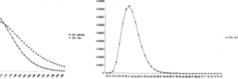
The capability of tracking the true D G P DV1 profile is very good; the estimated values of 0 correspond to an estimated peak at observation 270 (the true maximum

is at observation 269), and the estimated maximum value of DV1 is 0.00293 (whereas the true value is 0.0033). More generally, the entire estimated profile of DV1 is very similar to the true D G P profile, as is evident from figure 4.

These encouraging results are fairly robust with respect to simulated datasets with different DGPs, with different sample sizes, and different DV1 profiles. W e have encountered some difficulties in the estimation and the forecasting steps, when the degree of DV1 is particularly high, far from the ones that we consider reasonable and appropriate for real world phenomena.

5.3.2. A reduced EMU-1 1 model

Our second application is on real data: we use a simplified version of the constant price section of the EMU-11 model, in which we have eliminated the cxter- nal trade flows. It is, in fact, a HVAK model with 3 equations, GDI)

(U),

total investments (I) and private consumption (C). W e inserted only one exogenous variable, the terms of trade variable (TOT). The sample size is the same as in the original model (72 observations, from 1990:l to 1999:1), and the last four observations have been put aside to generate the usual set of control forecasts.

Figure 3 - Estimated m d true DV1 profileu. P i p m i - Estimated DV1 profile for the rcd~iced EMU-1 1 model.

(17)

As in the simulated data set example, we specify two different models, Model 1 and Model 2. Model 2 has 8, constrained to zero (no DVI), while Model 1 allows for DVI. In the case of Model l , the initialisation for the vector 8 reflects a priori beliefs on the transition process; our beliefs in this respect are that the transition started in 1990:l (observation 41), with the German i~nification process, and reached its maximum intensity at the end of 1993 (observation 56), alter the big currency crises that hit the European economies in 1992 and 1993. These hypoth- eses are accommodated by inilialising 8, = 0.0000001, C)? = 1.6, 8, = 0. l. The esti-

mated DV1 profile is reported in figure 5.

The advantages of dealing with a IIVI model are evident bp looking at the RIC criterion values for the two nloclels (table 8): Model 1 BIC is -2089.5, while Model 2 has -2033.08.

In general, the evidence gathered with this exercise leads us to make the following observations.

1 . In the gradual convergence towards EMU, the area-wide aggregates and their interrelations have been characterised by some major changes.

2. W e note that the traditional time varying parameter BVAR mechanism is not fully capable of modelling these transition phenomena. This fact can be used to explain some of the less than fully satisiactory properties of the EMU-11 models presented in the previous sections of this paper

3. The empirical evidence confirms that our procedure can be seen as a sensible solution to the problem.

4. Our a priori beliefs concerning the DV1 process are substantially modified by the data. In fact, the 0 hyperparameters obtained by numerical optimisation

(8, = l.3e - 007; O2 = 6.97; 8, = 1.01) locate the DV1 peak at 1991:3 (observation

37), whereas we originally thought that the maximum would be at observation 56 (1993:4). From 1991:3 on, the phenomenon gradually decreases, and it vanishes completely after the first half of 1994 (observation 58).

Summing up, the two experiments we have run confirm the usefulness of modelling gradual transition processes via time varying parameter schemes which are more articulated than the one of the standard BVAR approach. Our proposal in this respect, which is characterised by a DV1 mechanism governed by a small set of hyperparameters, is preferable to the traditional BVAR parameters evolution scheme on a closed economy, stripped down version of the KVS section of the EMU-11 model.

Considering each endogenous variable, we note that the Y and I forecasts are the ones that show the biggest improvements with respect to the no-DV1 model. In our view, this is quite interesting since we have seen in section (4) that the investment equations had the worst properties in the fully fledged, no DVI, EMU-11 model.

(18)

In this paper, we present a quarterly forecasting model for the the EMU-11 economies considered as a single country. The model has two sections: a constant price variables section and a section dealing with deflators. The model is a time varying parameter BVAli model which shows generally good forecasting performances and a good ability of tracking turning points without delays. Its forecasting performances, as measured by Theil's U indexes are largely superior to those of a non-Bayesian VAR model. In particular, on some crucial variables, such as G D P , consumption, exports, and inflation, the forecasts are particularly satisfactory.

The estimated models present some problems: the forecasting performances are not particularly brilliant for certain variables, such as construction investments and PPI. Moreover, the forecasting properties are very sensitive to the calibration of certain hyperparameters, and not robust with respect to the addition of new observations. Our interpretation of this problem is that the European economies have entered into a gradual transition process that has been revealed by a sudden wors-

ening of the forecasting performances of the models based on the traditional time varying parameter approach.

Taking all these things into consideration, in the second part of this paper we present an innovative method for handling parameters variability in a KVAR approach. We show that our procedure has good properties, by using two different applications. The first one is based on simulated data, and the second one on a

stripped down version of the EMU-11 model.

Some lines of research are at the top of our agenda. As for the EMIJ-11 model, we need to carefully assess the sensitivity of the model with respect to different scenarios by producing real out-of-sample forecasts. As regards our DV1 proposal, we still have to apply it to the fully fledged version of the EMU-11 model, and see how it works for that application. Moreover, we have to investigate the possibility of modelling the DV1 with different functional forms.

A further evolution is that of moving to a fully Hayesian approach, based on a

hierarchical structure, to be analysed by means of MCMC techniques, as in Amisano and Serati (2000).

Dipnrtinzento rli Scienzc cconomiche [Jniversiti di B r m i a

Paper presented at the Session: "Econometric methods for nlacroeconornic and financial forecasting", XI, Annual Scientific Meeting, Italian Economic Association, Ancona 29-30 October 1999. T h e authors wish to thanli Carlo Giannini, Jack Lucchetti, Ilicardo Mestre, Daniele Terlizzesc and seminar participants at the European Central Bank, Frankfurt. W e are particularly grateful to Elena Lizzoli for her invaluable collaboration.

(19)

RVAR modeh andforeca~tzng a yuatterly moddfot the ETJ-l1 69

REFERENCES

G. AMISANO, M . s r m u l (2000), tinemployment persistence in Italy. A n econometric analysis with multivariate timc va~ying parameter models, mimeo.

c;. ALIISANO, M. SF;,'.KATI, (:. C I A X N I S I (1997), l'ecnicke R V A R per lu costsuzione di rnodelli previsivi mensili e trimestmli, "Temi di discussione del Servizio Studi della Danca d'ItaliaW, n . 302.

!.M. i ~ t ; ~ n ~ ~ i t u o , A.F. S M I T I I (1994/, Bayesian Thcoyp, Wilcy, New York.

r. IMKEII 11978), Inflc~tion folrcasting with Bayesian 17AR models, "Journal of Forecasting", 17, pp. 147-165.

5 , (,I m , F . (;RLILNII~.II(; ( 1975), Hierurchical analysis of S U R models with extensions to co~-ielattd serial errors and time-zlaryiny paranzetcr models, "Journal of Econometrics", 68, 2, pp. 337- 360.

T . F . C O O L . ~ (1984), Comment to: Doan, l : , R . B . Litterrnan and C. Sirns, "Econometric Re-

views", 3, pp. 101-103.

,I.. noAh, ii. I r r r r i n h i ~ ~ , c , s l h l s (1984), Fo:01~casting and condition~il projections using i~alistic prior dist~ibutions, "Econometric Reviews", 3 , pp. 1-100.

1. ( ; F . ~ ~ E K E (1999), Using simulutior~ methods for Bayesian cconornetric nzodellirg: infcwnce, de- velopmont and comnzunication, "Econometric Reviews", 18, pp. 1-74.

J . I I ~ ~ M I I TON (1994), Time sesies analysis, Princeton University Press.

G. I.NX;RTN (1978), Mul;l.ov q i m c models for. mixed distributions and switching re~ressions,

"Scandinavian Journal of Statistics", 5, pp. 81-91.

R.B. I . ~ I .I.ERXIAS (LW')), l'cchniques offor.ecasting using vector autowgrexsions. "Federal Reserve Bank of Minneapolistextit", Working Paper, n. 115.

R . R . LITYKRMAN (1986), Forecasting wit11 Bayesian vector autoregws~ion - four years of experi- ence, "Journal of Business and Economic Statistics", 4, pp. 25-38.

F . X l h L l S V A I T ~ (1984), Comnzcnt to: Doun, 7'., R . B . Littcwzan and C. J'inzs, "Econometric Re- views", 3, pp. 113-117.

( : . A . SlM5 (1989), A nine vur.iabk probabilistic macroeconomic forecasting model, " I k k r a l reserve bank of Minneapolis Discussion paper", 11.14.

(:.(:.A. \Y'INI)~:R (1997), O n the cor~strziction of European ilwa-wide aggqates, "Irving Fisher Committee Bulletin", l , November, pp. 15-23.

AlodelIi A V A R e previsione: un model/o tsirnestde pes Z'lJhlE a 11 paesi

(Juesto lavoro it dedicato alla costruzione c alla ralutazione di un model10 previsivo tri- mestrale, appartencntc alla famiglia dei VAR bayesiani (RVAR), per il gruppo degli I l paesi aderenti all'unione Monetaria Europea IIJME) trattati come un unico paese. I n quests fase iniziale e transitoria del processo di completamento dell11JMF,, I'eroluzione d i molte variabili economiche t: caratterizzata da turbolenze e numerose relazioni macroeoconmicl~e sono af- flitte da instabiliti strutturale. Per questi motivi, i modelli utilizzati in questo lavoro sono modelli RVAR a paramctri variabili. Ad ogni modo, a fronte delle buone proprieti previsive d i questi modclli, rinlangono ancora segnali di una qualche loro parziale inadeguatezza. Alla luce di tali segnali, nella seconda partc del lavoro presentiarno im approccio innovative si~lla base del qualc la tradizionale metodologia BVAR a parametri variabili viene estesa c modifi- cata: I'intensiti di variazione dei parametri viene governata per mezzo di una matrice di varianza e covarianza dei termini d'errore dell'equazione di stato anch'essa rariabile nel

(20)

7 0 G. Amirurw, ilf. Semti

tempo. C:ib i. possihile ampliando (in misura minima) la dimensione dello spazio iperpara- metrico. L'evidenza empirica, prodotta sia sulla base di dati simulati, sia nell'amhito di una

r iante

version6 ristretta del model10 sull'UME a 11 paesi, seppur preliminare, appare i n c o r a g ' per quanto riguarda l'efficacia della nostra proposta.

SUMMARY

BVAR models and fotecastzng: a quarterly modcl for the Ehlli- I 1

This paper deals with the cos~ruction and evaluation of a quarterly forecasting BVAR model for the EMU-11 countries treated as a siilgle country. I n the current stage of EMU completion, most variables are aifectcd by turbulences, and many macroeconomic relationships are characterised by structural instability. For this reason, the I'orecastitlg models ~ l s e d in this paper are time varying RVAR models. There are still signs that the models me have estinlated are affected by some limitations, in spite of their good forecasting properties. In the light of this, in the sccond part of this paper W present an innovative approach in

which we extend the RVAR time varying parameter methodology: the intensity of pararn- eter variation is governed by a time varying variance covariance matrix of the state equation error tcrms. This is achieved by slightly increasing the dirnensionality of the hyperparameter space. WC show some preliminary, encouraging evidence on how this proposal works, based on simulated data and o n a restricted version of the EMIJ-11 model.