Investigation on energy efficiency for servo control applications

ALMA MATER STUDIORUM - UNIVERSITÀ DI BOLOGNA

SCUOLA DI INGEGNERIA E ARCHITETTURA

DIPARTIMENTO di

INGEGNERIA DELL’ENERGIA ELETTRICA E DELL’INFORMAZIONE “Guglielmo Marconi”

DEI

CORSO DI LAUREA IN INGEGNERIA DELL’ENERGIA ELETTRICA Tesi di Laurea Magistrale

in

AZIONAMENTI ELETTRICI per APPLICAZIONI INDUSTRIALI

INVESTIGATION ON ENERGY

EFFICIENCY FOR SERVO CONTROL

APPLICATIONS

CANDIDATO:

Simone Morini

RELATORE:

Prof. Angelo Tani

CORRELATORI:

Ing. Loredana Matea

Prof. Luca Zarri

Anno Accademico 2015/2016

To my parents and their inspiring curiosity

<<The Buddha, the Godhead, resides quite as comfortably in the circuits of a digital computer or the gears of a cycle transmission as he does at the top of a mountain or in the petals of a flower.

To think otherwise is to demean the Buddha, which is to demean oneself.>> Robert M.Pirsig, “Zen and the art of motorcycle maintenance”

CONTENTS

Abstract in lingua italiana………..

I

Acronyms and abbreviations………..

II

List of figures and tables………

IV

Chapter 1 Introduction to Servo drives………...

1

1.1

Problem background………..

1

1.2

Content of the thesis………...

5

1.3

Purpose of the project………

7

Chapter 2 Theoretical evaluation of the losses………...

9

2.1

Inverter Losses………...

10

2.1.1 Conduction losses………..

10

2.1.2 Switching losses……….

13

2.2

Motor Losses………..

17

2.2.1 Copper losses……….

18

2.2.2 Iron and magnet losses………...

19

2.2.3 Mechanical losses……….

26

2.3

Gearbox losses………...

27

2.3.1 Meshing losses………...

29

2.3.2 Bearing losses………

30

2.3.3 Seals losses……….

31

Chapter 3 State of art of efficiency in Servo drives………

34

3.1

Inverter………...

35

3.1.1 Materials for Power electronics……….

36

3.1.2 Topology for Power electronics……….

37

3.1.3 Control and modulation techniques………...

39

3.2

Electrical motor………..

42

3.2.1 Materials for electrical machines………...

47

3.2.2 Structure for electrical machines………

49

3.2.3 Control for electrical machines………..

54

Chapter 4 Efficiency maps for Servo motors……….

62

4.1

Method to derive an efficiency map for Servo Drives...

63

4.2

Results for BMD 65………...

68

4.3

Results useful for the experiment………...

72

Chapter 5 Experimental validation……….

77

5.2

Results………

84

5.2.1 Resistance measurement………

87

5.2.2 Efficiency calculation comparison……….

88

5.2.3 Inverter efficiency………..

91

Chapter 6 Sizing procedure including accurate efficiency

evaluation………...

93

6.1

Servo drives selection criteria………

94

6.2

Calculation of the required performance………...

98

6.3

Integration of efficiency maps in the selection………..

103

6.4

Application case: comparison of scenarios for hoist….

107

Conclusions………

115

I

ABSTRACT in LINGUA ITALIANA

Lo scopo del lavoro è stato migliorare la previsione del consumo energetico di applicazioni per servo controllo. La tesi è stata proposta e supportata dalla divisione Meccatronica di un'azienda locale. Un'analisi più accurata dell'efficienza in specifici cicli di lavoro, che portano i componenti a lavorare lontano dai punti nominali di funzionamento, può aiutare nella selezione ottima degli stessi e nel calcolo del loro costo operativo di vita.

L'analisi prende in considerazione particolari componenti quali inverter con controllo vettoriale, motori brushless a magneti superficiali e riduttori planetari a gioco ridotto. Questo tipo di componenti massimizzano la dinamica e la precisione del controllo. Le perdite più importanti vengono descritte teoricamente. Successivamente si presenta un'indagine sullo stato dell'arte dei più diffusi modi per ridurre le suddette perdite. Per il motore elettrico viene elaborato un algoritmo in grado di ricavare delle mappe di efficienza, ovvero il valore delle perdite e dell'efficienza in ogni punto del diagramma coppia velocità. L’algoritmo considera diverse temperature di funzionamento cercando di predirle dal tipo di funzionamento operativo. Laddove venga misurata la resistenza e la temperatura della cassa del motore si possono ottenere informazioni più dettagliate sulla temperatura degli avvolgimenti e si possono quindi calcolare le perdite Joule con maggiore precisione.

L'obiettivo è fornire uno strumento di facile implementazione, come un'equazione polinomiale, con cui si possano calcolare le perdite del componente per ogni particolare fase del ciclo di lavoro. Inevitabili approssimazioni che non considerano le reali condizioni operative devono essere verificate per validare la correttezza del metodo. E' stato condotto un esperimento in cui si calcolano le perdite di un motore flangiato ad un riduttore. Nel calcolo delle mappe infatti i componenti sono considerati da soli in una differente situazione di scambio termico. Le misure reali condotte confermano un errore nella stima dell’efficienza da parte delle mappe del motore e del riduttore soprattutto ad alta velocità quando le temperature delle casse sono alte. Si nota inoltre come le perdite sull’inverter sono comparabili con quelle degli altri componenti e si consigliano ulteriori analisi che esulavano dagli scopi di questo lavoro.

Per concludere si presenta l'integrazione del metodo nella selezione ottima dei componenti che usa una più accurata previsione delle perdite e quindi dei consumi energetici annui.

II

ACRONYMS

Total Harmonic Distortion Total Cost of Ownership Pulse Width Modulation

Finite Element Method/Analysis Computational Fluid Dynamics Permanent Magnet

Permanent Magnet Surface Mounted Interior Permanent Magnet

Space Vector Pulse Width Modulation Discontinuous Pulse Width Modulation Wide Band Gap

Field Oriented Control

Bonfiglioli Mechatronic Research Mechatronic and Drives Solutions Voltage Source Inverter

Maximum Torque per Ampere ratio

SYMBOLS

Pi Active Power [W]

Wi Energy [J]

Vi Phase Voltage [V]

Vce sat Collector-Emitter Voltage [V]

Io Output current [A]

Rs Stator Resistance [Ω]

J Current density [A/m 2_]

Is Stator phase current [A]

Θ Temperature [K]

Τ Torque [Nm]

θ m Angular position (mechanical) [rad]

f Frequency [Hz]

Bm Flux density [T]

σ Conductivity [Si/m]

ρ Resistivity [Ω m]

III

μι Magnetic permeability [H/m]

F Force (radial) [N]

v Velocity [m/s]

δ Air gap length [m]

n Rotational mechanical speed [rpm]

p Number of pair poles

D Diameter of the stator [m]

H Magnetic field [A/m]

e i Electromotive force [V]

ω m Rotational speed [rad/s]

ω Pulsation [rad/s]

Jm Inertia of the motor [Kg/m2]

J

Ls Inductance of the Stator [H]

Mse Mutual Inductance [H] φ em Magnetic Flux [Wb] τ Pole pitch [m] Pm Permeance [H] N Number of conductors Xs Stator Reactance [Ω] Vpk Peak Voltage [V]

Ipk Peak Current [A]

Rpp Phase to phase resistance [Ω]

i Ratio of reduction

r Inertia mismatch

JL Inertia of the load [Kg/m2]

IV

LIST OF FIGURES and TABLES

Fig. 1.1: “Total cost of Ownership of a Pump”

Fig. 1.2: “Effect of an improvement in efficiency on TCO” Fig. 1.3: “Wasted energy in the mechatronic chain”

Fig. 1.4: “Possible choice of type of components and their nominal efficiency” Fig. 2.1: “Losses distribution scheme”

Fig. 2.2: “Typical structure of VSI inverter” Fig. 2.3: “Mid-level detailed IGBT model” Fig. 2.4: “Structure of IGBT”

Fig. 2.5: “Simplified ON state model” Fig. 2.6: “I-V chart for IGBTs”

Fig. 2.7: “Switching and on state behaviour approximation” Fig. 2.8: “Detailed evolution of turn on of the IGBTs” Fig. 2.9: ““Detailed evolution of turn off of the IGBTs” Fig. 2.10: “Energy losses in the switching vs current” Fig. 2.11: “Typical structure of PMSM motor”

Fig. 2.12: “Different hysteresis cycle for ferromagnetic materials” Fig. 2.13: “Typical hysteresis cycle of an iron electromagnet” Fig. 2.14: “Induced magnetic field and flux distribution” Fig. 2.15: “Benefit of a laminated core against eddy-currents” Fig. 2.16: “Eddy currents on PM”

Fig. 2.17: “Structure of a planetary gearbox” Fig. 2.18: “Classification of gearbox losses”

Fig. 3.1: “Several benefits of the wide band gap materials in comparison with Silicon” Fig. 3.2: “Reduction of the widt of drift region in SiC devices”

Fig. 3.3: “General topology of a 3 level inverter NPC” Fig. 3.4: “Space vector operation”

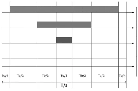
Fig. 3.5: “traditional SVPWM with symmetrical pattern and with both zero vectors” Fig. 3.6: “DPWM30° operation and modulation ratio”

Fig. 3.7: “DPWM60° operation and modulation ratio” Fig. 3.8: “PMSM motor”

Fig. 3.9: “PMSM motor and IPM motor”

V

Fig. 3.11: “MTPA until the base speed”

Fig. 3.12: “Operational limits on torque speed plane” Fig. 3.13: “Energy density of most common magnets” Fig. 3.14: “Distributed and concentrated windings” Fig. 3.15: “Pulsating torque for PMSM machine” Fig. 3.16: “Reason of the cogging torque”

Fig. 3.17: “Cogging torque waveform”

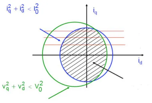
Fig. 3.18: “Blondel diagram for synchronous machine” Fig. 3.19: “Quadrature of armature and excitation field” Fig. 3.20: “Rotor oriented control”

Fig. 3.21: “General operation of FOC for PMSM motor”

Fig. 3.22: “Review of sensorless control for speed/position estimation” Fig. 4.1: “Algorithm used for efficiency map generation”

Fig. 4.2: “Equivalent circuit with resistance for iron losses and leakage current” Fig. 4.3: “Efficiency map for S1 for small motor, nominal torque 1.7Nm” Fig. 4.4: “Total losses map on torque speed diagram”

Fig. 4.5: “Joule losses map” Fig. 4.6: “Iron losses map”

Fig. 4.7: “Mechanical losses map”

Fig. 4.8: “Efficiency map for peak operation of BMD 65”

Fig. 4.9: “Efficiency map for BMD 145 in S1 operation”

Fig. 4.10: “Main losses for planetary gearbox divided in load dependent and independent”

Fig. 4.11: “Iterative procedure to find temperature for gearbox losses calculation”

Fig. 4.12: “Losses map for gearbox TQ090_i5” Fig. 4.13: “Temperature map for TQ090_i5”

Fig. 5.1: “Experimental setup: combination of BMD145 and TQ090” Fig. 5.2: “Scheme of the measurement setup”

VI

Fig. 5.4: “Data sheet of the PMSM motor used in the experiment” Fig. 5.5: “Operational limits for the series of motor selected”

Fig. 5.6: “Data sheet of the gearbox used”

Fig. 5.7: “Set up of the experiment: motor + gearbox under test, torque meter and generator motor”

Fig. 5.8: “Evolution of the temperature on the frame of the motor”

Fig. 5.9: “Working points on the torque speed diagram for motor and inverter”

Fig. 5.10: “Working points on the power speed diagram for the motor and inverter”

Fig. 5.11: “Working points on torque speed diagram for the gearbox”

Fig. 5.12: “Resistance extrapolation”

Fig. 5.13: “Efficiency of the inverter for different load”

Fig. 6.1: “Factors that influence the mechanical resonant frequency”

Fig. 6.2: “Needed parameter for the sizing procedure”

Fig. 6.3: “Gearbox selection method”

Fig. 6.4: “Efficiency characterization for motor in the professional software” Fig. 6.5: “Gearbox efficiency characterization in the professional software” Fig. 6.6: “Scheme of the component for hoist application”

Fig. 6.7: “Load and speed profile required”

Fig. 6.8: “Motor and drive working points for scenario 1” Fig. 6.9: “Motor and drive working points for scenario 2”

Fig. 6.10: “Economical comparison of the two scenarios for hoist” Fig. 6.11: “Working points on the efficiency maps for scenario 1” Fig. 6.12: ““Working points on the efficiency maps for scenario 2” Table 3.1: “Sum of strategies for servo motor”

Table 4.1: “Losses dependence on torque and speed for PMSM motor” Table 5.1: “working points of the experiment”

VII

Table 5.2: “Resistance measurement and overtemperature calculation” Table 5.3: “Losses calculation comparison”

Table 5.4: “Efficiency comparison” Table 5.5: “Motor losses separation”

Table 5.6: “Comparison after correction of the Joule losses” Table 5.7: “Inverter losses”

Table 5.8: “Inverter efficiency”

Table 6.1: “Operational limits of electrical motors” Table 6.2: “Results with the proposed method”

Table 6.3: “Comparison between the proposed method and the professional software”

Table 6.4: “Comparison between the professional software and the results form experiment”

Table 6.5: “Main parameters for the two different scenarios”

Table 6.6: “Results for scenario 1”

1

Chapter 1

INTRODUCTION TO SERVO DRIVES

This chapter introduces the reason and the purpose of the project. Servo drives include many different types of application characterized by the need of high dynamic and position accuracy. The choice of the size of the components nowadays does not include accurate efficiency analysis but it focuses mainly on the mechanical strength, robustness and thermal loadability. Due to the increasing importance of efficiency, this work aims at a more accurate analysis of the efficiencies of the components in the varying working cycle. This kind of approach allows the optimization in the selection of the sizes also from energy consumption prospect.

1.1 Problem Background

After Kyoto Protocol, new law about Minimum Efficiency Standard for electric motors and a grown sensitivity of industries and people to environmental issues, the efficiency of the mechatronic solutions became a crucial point of the field. The product that succeeds, combines high performance, high dynamic response, high density to reduce the size and eventually high efficiency.

Besides the need to save energy for the grown green consciousness and to contribute to fight the climate change, being efficient might mean great savings in the electricity bill of the companies.

This work was proposed, encouraged and assisted by the Industrial Mechatronic Drives Solutions division of Bonfiglioli Riduttori s.p.a..

It is determining for this field of application being able to provide to the customer efficient products and therefore an efficient drivetrain.

Nowadays the initial cost of a product is not considered anymore so important but customers look at the Total Cost of Ownership (TCO). This parameter is the sum of the cost of the product in its entire operating cycle. Fig. 1.1 shows an example of TCO for a pump.

The Fig. 1.2 depicts, instead, that a little improvement in the efficiency can provide a relevant reduction of the total cost permitting to save money on the long period with a slightly bigger initial cost.

2

FIGURE 1.1: TOTAL COST OF OWNERSHIP OF A PUMP [1].

FIGURE 1.2: EFFECT of AN IMPROVEMENT IN EFFICIENCY on TCO [1].

Inside the Industry application the company has separated the business units dedicated to Power Transmission solutions and the Mechatronic ones. The project was proposed by this latter that presents the solutions with the highest efficiency. The author received support from the business unit MDS (Mechatronic and Drive Solution). For this reason, the products considered are the ones designed, built and sold by this division of the company.

3

The solutions considered are SERVO drives and combine a Servo inverter with an optional Sensorless control, a Permanent Magnet Surface Mounted motor with high torque density and a high precision planetary gearbox. Each component dissipates part of the energy in heat that does not contribute to the power transmission as in Fig. 1.3.

FIGURE 1.3: WASTED ENERGY IN THE MECHATRONIC CHAIN [1]. Some examples of application of Servo Drives are:

• Machine tools • Packaging • Conveyors • Cranes and Hoist • Textiles

• Robotics

• Paper and Paperboard • Electronics Assembly • Semiconductor

4

To properly evaluate how and where the energy is being wasted in the entire chain (Variable frequency converter- Electrical Motor- Gearbox) it is important to watch the components altogether. The gearbox often may be the weak point. Since the global efficiency is the product of the efficiency of the 3 products if one of them has a very low efficiency, improvements in the others would be less effective.

High precision planetary gearbox, due to their technology and their construction process, allows higher input speed and higher efficiency. Thus, for a Servo axis the size of the motor is usually reduced in respect of industrial application. This reasoning is valid with types of gearboxes with low efficiency as the worm gears or generally with older or less expensive industrial gearboxes that have nominal efficiency between 50% and 90%. The planetary gearboxes have instead a nominal efficiency over 95% therefore in Servo drives (or whenever a high efficiency gearbox is chosen) all the 3 components matter as suggested in Fig. 1.4 where typical products for Industrial applications are depicted along with their nominal efficiency.

Therefore, the sizing procedure plays the crucial role in the optimization of cost and energy consumption.

Usually the efficiency point of view is still seen as marginal in the selection of the components. Often, to avoid complicated issues further discussed, the nominal efficiency of the component is assumed constantly or slightly dependent on the speed or torque. However, when each component is furtherly investigated it is undeniable that the losses of the electrical motors and of the gearboxes depend on both torque and speed. Therefore, considering the nominal efficiency as a valid value in many working points, which are different from the one in which that value is calculated, may be incorrect. The efficiency with low percentage of the nominal torque and at very low speed may vary significantly in comparison with the nominal one. A selection that aims to decrease only the weight or the cost (as it is common) may end up in selecting a very low efficient drivetrain for the specific cycle asked by the load. Selecting the components that run in working points with low efficiency might increase the TCO.

A method to derive a detailed characterization of the efficiency of these two components is proposed. A similar strategy was not developed for the inverter but the results from experiment demonstrate that the efficiency of inverter also drops at low speed. This suggests the need of characterization also for the converter and it should be verified in future works. The focus of the thesis is mainly on the electrical motor since the field of the

5

study of the author is electrical engineering. Moreover, the ratio of the gearbox is the main degree of freedom of the selection so when the ratio changes the size of the motor, the speed and the torque asked change with it.

FIGURE 1.4: POSSIBLE CHOICE OF TYPE OF COMPONENTS AND THEIR NOMINAL EFFICIENCY [1].

Then, it can be said that with the same number of stages of reduction the same type of gearboxes shows similar efficiency results. Thus, it seemed reasonable that the optimization of the ratio was made considering mainly the efficiency of the motor.

1.2 Content of the thesis

Chapter 2 describes the main types of losses and their physical reasons. The converter frequency has mainly conduction and switching losses. Conduction losses are proportional

6

to current and so to the torque asked by the load. Switching ones are basically proportional to the switching frequency chosen and so they may be linked to the desired quality of the current (high switching frequency guarantees a lower THD).

Electrical motors dissipate Joule losses (or Copper losses) due to the finite conductivity of the metals and Iron losses on the stator and rotor core. These last ones are a particular complicated subject. Moreover, losses on the magnets may be significant and windage losses should be considered.

Gearbox losses are even more difficult to be calculated precisely since in the planetary gearboxes independent load losses are more significant. These losses are the results of fluid dynamical events of the oil and the air. The operating condition of the gearboxes change the temperature and so the viscosity, CFD analysis are needed. Furthermore, meshing losses are due to friction and they are load dependent. Also, bearing and seals losses are included. Chapter 3 includes a review of the state of art of inverter and PMSM motor. Different strategies to optimize the efficiency and the performance are presented trying to focus on the most popular techniques in the industry and the most attractive improvements.

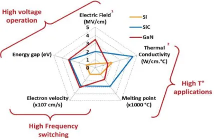
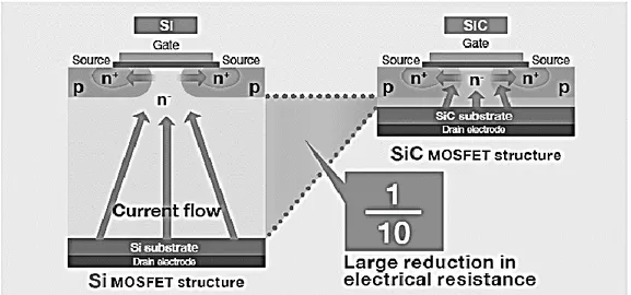
For the inverters, emerging wide band gap (WBG) materials seem very promising and offer several benefits. More complex topology as multilevel inverter (as Neutral Clamp Pointed 3 level converter for instance) may improve the quality of power conversion. Eventually peculiar choice in the modulation technique of the Pulse Width Modulation may decrease the switching losses without compromising the THD.

Electrical motors present nowadays several different technologies but for the Servo drives application the Permanent Magnet motors are used to maximize the torque density and Maximum Torque/Ampere ratio. Briefly the equations of the equivalent model in the synchronous reference frame are presented to investigate the operational limits. Then considerations about the materials, the structure and the control are developed. The materials are quite consolidated in the windings while iron powder or iron alloy may improve the torque density. The magnets as Neodymium Iron Boron are definitely the most powerful on the market. Insulators also play a key role.

Furthermore, the structure of the PMSM motor can be optimized to increase the power density with a high number of poles and with the adoption of the concentrated windings. Nevertheless, the issue about the pulsations of the torque are introduced and the most common method to have a sinusoidal waveform of EMF and to reduce the cogging torque are mentioned. Field Oriented Control optimizes the relative position of the magnetic fields

7

producing the torque and nowadays Sensorless control is becoming more and more popular because it avoids the use of speed measurement tools.

Chapter 4 deals with the method employed to derive the efficiency map for the electrical motor. The efficiency is plotted on the torque-speed diagram and it can be therefore simplified in a polynomial function of the variables. The main principle is to consider that copper losses are proportional to the square of the torque while iron losses are somehow proportional to the speed of the motor. The accuracy of the map depends on the level of detail of the information used. The author received from Bonfiglioli Mechatronic Research several data of FEM simulations of some motors of the company. Thanks to this detailed information a script generates the map and a prediction of the efficiency in each working point is available. A case is presented showing the division of the total losses between copper, iron and mechanical ones.

Chapter 5 includes the description of the test conducted in Bonfiglioli Mechatronic Research. Since the map of the motor and of the gearbox (that was received from the author from BMR) are validated with the component alone, the values of efficiency are expected to decrease when the components are flanged together. The heat exchange in fact is very different and the temperature would increase. The test analyses the real efficiency in the real operating condition. The error committed by the prediction of the maps is quantified and justified. Moreover, a verification of the maximum overtemperature of the windings is presented. Finally results of the inverter efficiency are shown.

Eventually chapter 6 focuses on an improvement in the optimization of the ratio of the gearbox with the more accurate information obtained about the efficiency. The sizing procedure has to take into account different selection criteria and so far the mechanical strength and thermal loadabillity are the most investigated. Since the increasing accuracy of the efficiency, a more reliable prediction of the energy consumption may be achieved. Therefore, after presenting the main matters in the selection of the components and in the choice of gearbox ratio, the efficiency maps are integrated in the method.

An example is presented to show that the minimization of the energy consumption might not coincide with the minimization of the initial cost.

1.3 Purpose of the project

The purpose of this project was mainly practical: it aimed to give a simple and effective tool to Customer Application engineers to analyse the efficiency of different scenarios

8

during the sizing procedure. Especially in Europe, where the cost of energy is higher the Total Cost of Ownership of a mechatronic solution deeply depends on its own energy consumption and a bigger investment in initial cost may be repaid back in a certain time. The demanding improvement was enhancing the accuracy of the efficiency calculation paying attention to consider the exact working cycle in which the components will work. To correctly calculate losses on the mechatronic solution in a general approach valid for a wide range of applications the losses on each component are investigated. Due to the complexity of the subject it is not convenient to try to obtain a detailed model of equations that would calculate the losses for each torque and speed. The real efficiency in fact is strictly linked to the operating and environmental conditions in which the solutions will work. A precise calculation is not completely possible and all the results are an approximated prediction of the real efficiency. Therefore, developing a very complex algorithm able to model all the losses would present a great computational effort and anyhow the accuracy of the prediction is quite poor.

Beside the operating and environmental conditions the first approximation made in the development of the efficiency map is considering the component alone. When the component is working in the real condition, instead, the gearbox and the motor are flanged together and the quality of the heat exchange is decreased and so the efficiency may vary. The temperature inside the gearboxes or the temperature of the windings are fundamental information to properly estimate the efficiency but they are also very difficult to be predicted precisely and dynamically. Moreover, the quality of heat exchange depends on the temperature itself and makes the calculation iterative. The test described in Chapter 5 aims to quantify the difference in the efficiency calculation between these two conditions. The tool developed should be able to offer a rapid analysis of how the efficiency varies between different scenarios. The intent of the author was to find a proper trade-off between an academic approach with the typical more practical approach of a company. While the first needs mathematics and physics phenomenon interpretation, the second may be based often on experience and rules of thumb. The main issues of the mechatronic are investigated more deeply where the practical approach may lack of accuracy.

Reference Chapter 1:

9

Chapter 2

THEORETICAL EVALUATION OF THE

LOSSES ON EACH COMPONENT

To discuss about the efficiency of the entire drive solution the first step is to deeply understand where and how part of the energy is lost. Several non-ideal behaviours of the nature cause different losses, instead of transmitting the entire power to the next component a percentage of that is dissipated in heat without contributing to the transmission. In this chapter the most relevant losses are described.

In order to design and control our devices focusing on their efficiency it is crucial to know the physical phenomena that cause the losses. The scheme in Fig. 2.1 summarizes the losses described in this chapter. The choice of the motor will be explained later.

FIGURE 2.1: LOSSES DISTRIBUTION SCHEME

.

The calculation of the losses of each component has a very broad literature. This topic, in fact, is widely investigated for many reasons. Firstly, the thermal analysis needs some information about the heat produced by the components. Moreover, the optimal design of the dissipation system of the components needs to know the amount of losses produced in the nominal point.

10

In the chapter a brief description of the physical reason is followed by an analysis of the most common method calculation of each type of loss. Losses in the iron and in the lubricant, require FEM and CFD calculation respectively. As previously mentioned, for the purpose of the project these complicated method calculations were not investigated deeply. Moreover, indirect methods to derive the iron losses are often used to avoid the computational effort. For these reasons, in the chapter only the analytical formulas are presented.

2.1 Inverter Losses

The structure of a VSI inverter is the one shown in Fig. 2.2:

FIGURE 2.2: TYPICAL STRUCTURE OF VSI INVERTER.

Since the maximum junction temperature should not be reached at any time, the losses produced by a converter frequency are studied to select the proper components checking the thermal loadability. There are different types of losses that need to be considered:

• conduction losses occurring in the ON state

• switching losses in any turn-on/off of the components • off-state (stand-by) losses (not discussed)

2.1.1 Conduction Losses

The conduction losses are mainly due to the finite resistivity of Silicon and to the presence of the internal resistances both on the diodes and the IGBTs. The conductivity is the product of the number of free carriers times the electrical mobility (μ) that describe the tendency of

11

electrons to be moved. The number of free electrons in the semiconductors varies with the temperature, while instead it is constant for metals and insulators. At the environmental temperature, a proper doped silicon (pn junction) can be considered already a good conductor over the threshold voltage. The mobility instead can be manipulated in the design of the semiconductors. It depends mainly on the impurity level, temperature and electrons or holes concentrations. The internal resistance of the power devices is linked to the width of the Drift region (n- region in Fig. 2.4), that presents a lower density of free carriers to provide a higher breakdown voltage. Fig. 2.3 shows an equivalent circuit of IGBT.

IGBTs are widely used in many kinds of power frequency converter. They combine the advantages of Mosfets in the switching behaviour with the better ON state behaviour of bipolar transistors. IGBTs present in fact, very low on state voltage drop along with a superior current density at high breakdown voltage. Moreover, they require low power drive circuit thanks to the MOS input. All in all, they have a wider Safe Operating Area in comparison with both the other 2 traditional devices (Mosfet and BJT). The value of that internal resistance is about order of mΩ and it doesn’t change drastically at high voltage breakdown like in the Mosfet [1].

The value of the internal resistance (called Ron) increases with the width of the drift region. To achieve higher breakdown voltages the width should be larger so a trade-off is in any case needed in the design.

12

FIGURE 2.4: STRUCTURE OF IGBT.

The conduction losses on the rectifier are the power dissipated by the diodes. To calculate them the same approach that will be discussed for the inverter can be used. Both diodes and IGBTs in fact present a similar ON state behaviour with the drop voltage due to the threshold of the junction plus the internal resistance.

Different methods are proposed to calculate conduction losses on the inverter [2][3]. Different level of detail of the model of the devices are also proposed but basically, they all require specific data that are not provided in the Datasheets as the one depicted in Fig. 2.3.

However, from the I-V characteristic curve of the device it is easy to obtain the value of the internal resistance (Ron) that can be used in the simple but quite accurate ON-state model [2] shown in Fig. 2.5.

FIGURE 2.5: SIMPLIFIED MODEL OF ON-STATE.

Due to the dependence of the resistance on the junction temperature the right curve has to be chosen in the data sheet output characteristic shown in Fig. 2.6. The conduction losses can be calculated as in [1] as:

𝑃

=

∫ 𝑉

𝐼

𝑑𝜏=

∫ (𝑉

+

𝑅

𝐼

)𝐼

𝑑𝜏||T/D

13

WhereV D/T is the threshold voltage of the diodes or the transistors. τ is the period of time

in which the component considered is conducting. The IGBTs conduct both when the signal of the switch is 1 (upper one ON) and the phase current Ia is positive and when the switch is 0 (lower one ON) and the current is negative. Vice versa for the diodes.

An example of Data Sheets (from Infineon) with the static characteristics of IGBTs is shown in Fig. 2.6. From this chart, it is possible to derive a value for the internal resistance of the device. The junction temperature and the voltage of the drive gate change the internal resistance therefore they should be considered during the choice of the chart. As a result, the conduction losses are linearized by an internal resistance and by the threshold voltage. The value is multiplied by 3 to obtain the losses of the three legs since the same switching pattern, ac currents and voltages are applied to all the phases.

FIGURE 2.6: I-V CHART FOR IGBTs.

2.1.2 Switching Losses

The switching losses, instead, take place only in the time period in which the IGBTs or the diodes are switched. It is not possible to achieve a switching time equal to zero due to physical reason. The amount of losses becomes such important nowadays when the

14

converters use switching frequency up to Megahertz. Caused by different inherent delay of the components as the rise and fall time but also delay time (as reverse recovery and tail current time), switching losses correspond to the dissipation that occurs when both current and voltage are changing. Switching losses exist because in that interval the components have contemporary voltage and current very different from zero and it produces a power dissipation of V times I.

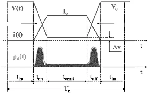
Generally, they can be calculated as: 𝑊_{𝑜𝑛/𝑜𝑓𝑓} = ∫𝑡𝑜𝑛/𝑜𝑓𝑓𝑣(𝑡)𝑖(𝑡)𝑑𝑡 0 =∫ 𝑉𝑐𝑒(𝑡)

𝐼

Fig. 2.7 shows an approximation of the evolution of the voltage and current.

FIGURE 2.7: SWITCHING AND ON-STATE BEHAVIOUR APPROXIMATION.

The physical reason that avoids an instant switch is the presence of a stored charge. The diode exhibits the phenomena of reverse recovery current that delays its turn off. In Data sheets the parameter Err describes this event. The IGBTs have a more complex structure but the major contribution to the delay times is due to its bipolar behaviour. In Fig. 2.8 and 2.9 the evolution of the turn on and off is depicted in a more detailed way. The delay time is clearly visible. The first, in Fig. 2.8c, is the drain source voltage in the turn on that slowly enters in its hard saturation area before the drop voltage reaches its final (saturation) value.

15

Instead, in the turn off behaviour the drain current (Fig 2.9b) exhibits the typical tail current of the bipolar behaviour: chargers are stored in the drift region and before stopping the conduction these carriers must be removed.

Generally, also for IGBTs an approximation is made between the two different slopes of the curve due to the MOS/bipolar behaviour.

As in [3] they can be calculated with approximation of the waveform of the Voltage and the current but the value of the parasitic capacitors are needed to calculate the constant time of the RC circuit and therefore the delay times.

A faster approach is however suggested in [2] exploiting data sheets that provide different value of the energy consummated by the process. From this value the switching losses can be easily determined with a good accuracy. The sign of the current and the duty cycle chosen determine different configurations and different paths of the current therefore all the possibilities must be considered.

16

FIGURE 2.9: DETAILED TURN-OFF OF IGBT.

The chart of Energy/collector current, shown in Fig. 2.10, is taken from a datasheet of Infineon and it presents respectively the total, turn on and turn off losses including the reverse recovery of the anti-parallel diode.

FIGURE 2.10: ENERGY LOSSES IN THE SWITCHING (ON, OFF, TOTAL) VS CURRENT.

17

Some points can be selected and fitted using a second order polynomial through the function Polyfit in Matlab as suggested in [2]. This permits to achieve an analytical expression of the dissipated energy function of the off-state voltage and of the collector current. A Simulink model and a code to simulate the duty cycle are also needed. After obtaining the proper function the total switching losses can be calculated knowing the level of the gate signal and the sign of the collector current. The calculation is iterated for every switching cycle using the turn on or the turn off losses for both the transistor and the diode. In [3] different suggestions are proposed. From the datasheet, also information about the condition test may be used, therefore the total energy losses are scaled with the change of Current, Voltage (Vce) and the value of the gate resistance as well as temperature.

𝐸𝑡𝑜𝑡 = (𝐸𝑜𝑛+ 𝐸𝑜𝑓𝑓) 𝑉 𝑉𝑡𝑒𝑠𝑡 𝐼_𝑐𝑒 𝐼𝑡𝑒𝑠𝑡 (2.3)

2.2 Motor Losses

The type of motor analysed as previously mentioned is the PMSM motor. Obviously with different motors the type of losses and their relevance can remarkably change [4]. In chapter 3 the main advantages of this kind of motors will be presented. This chapter only deals with the description of the losses. In comparison with the other most common choices, as Induction Motors, the rotor copper losses are removed. However, magnet losses may be more significant in the high-speed region in comparison with Reluctance (SynRel) motors or Interior Permanent Magnet motors. The typical structure of a permanent magnet surface mounted motor is shown in Fig. 2.11.

18

FIGURE 2.11: TYPICAL STRUCTURE OF PMSM MOTOR.

2.2.1 Copper Losses

The physical reason for the conduction losses is that none of the materials presents an infinite electrical conductivity at environmental temperature. The best conductors are typically metals and Copper or Aluminium are the most common ones thanks to their good mechanical properties, light weight, easy supply and almost stable price.

The metallic bond leaves some atoms free to circulate when an electrical voltage difference is applied. But, at the environmental temperature, the atoms already have their own vibration due to thermal (or kinetic) energy. While an electron is moving, it wastes part of its energy crushing with the other electrons around it. The resistance of metals increases with the temperature because the electrical mobility of electrons decreases due the increasing reticular vibration.

Moreover, as known, the skin effect can reduce the section involved in the conduction process therefore in the calculation of copper losses it is important to take into account the frequency of the current. In particular, for motors with a high number of poles it can be common to use high nominal frequency. This may reduce the skin depth to a value smaller than the radius of the conductor. The calculation for copper losses uses the Joule’s formula for the power dissipation:

𝑃

= 𝜌

𝑉𝑜𝑙

𝐽

𝑃

= 3𝑅

(𝛩)𝐼

19

Different dimensions or different number of conductors can modify the joule losses. Some considerations about the influence of the design on the copper losses are presented in chapter 3.

As known, the stator resistance increases proportionally with the temperature. Equation (2.5) is widely used to take into account the increase of resistance but also to verify the maximum temperature reached by the windings in the nominal working point. α is 3.93e-3 [K-1] for copper and 4.26e-3 [K-1] for aluminum. The second one is easier to be applied for different ambient temperature and it is considered for copper.

𝑅

= 𝑅

(1 + 𝛼𝛥𝛩)

𝑅_{𝛩𝑎𝑣𝑔}= 𝑅_20°𝐶(234.5 + 𝛥𝛩 + 𝑇𝑎𝑚𝑏) (234.5 + 20)

(2.5)

2.2.2 Iron and Magnet Losses

The issue about the iron losses is one of the historical problems of electrical engineering and research is still proposing improvements in efficient FEM calculation [5]. A high level of accuracy requires many resources and in Chapter 4 that deals with the calculation of the efficiency maps assumptions will be unavoidable. In [6] different methods are compared in accuracy and resources demand. To enhance the accuracy, the losses are divided between yoke and teeth because both contribute to hysteresis and eddy currents losses but the value of the flux density may be very different.

The phenomenon of ferromagnetism is linked to the magnetic permeability that describes the tendency of a material to be able to orient the magnetic momentum of its atoms in the same direction. Very few elements in the periodic table exhibit this quality. Inside a PMSM motor the phenomenon is exploited in different ways. The iron provides the proper path for the magnetic flux. It is necessary to have soft magnetic elements with a little cycle of hysteresis and little coercivity to avoid huge losses as seen in Fig. 2.12. While the permanent magnets, that is Neodymium Iron Boron, exhibit a very large cycle that provides a strong magnet with high saturation level, residual magnetism and coercivity (Hard ferromagnetic).

20

FIGURE 2.12: DIFFERENT HYSTERESI CYCLES FOR FERROMAGNETIC MATERIALS.

All the Iron losses are mainly due to the variability of the magnetic flux and they all depend on the frequency of the current that generates the magnetic field and therefore on the speed requested by the motor.

Commonly, the stator core losses are divided in hysteresis and eddy-currents losses. Someone adds extra current-losses, and investigations considering the increase with the harmonic content are presented in [8] [9]. The well-known Bertotti’s equation gathers these 3 terms. Moreover, rotor eddy-current losses should be considered, too. They can be placed specifically on the magnets or on the rotor steel and depend on the shape of the magnets and on the harmonic content of the air gap field. All in all, the iron losses can be divided as:

• hysteresis Losses • eddy-Currents losses

• additional eddy-currents losses • magnet and rotor losses

Concerning the stator core losses that are the sum of the first 3 terms of the list, it is worth to point out [7] that the division of the losses represents a difference in the scale of the magnetization. Hysteresis losses describe the localized jump of small domain walls due to the Barkhausen effect. Classical eddy currents are linked to a uniform change of magnetization throughout the sample and their path strongly depends on the dimensions and the shape. Finally, the scale of the additional eddy current losses is the domain walls and they don’t depend so much on the shape of the sample. From this consideration, the initial approach to have a reliable model is to divide the kind of losses on their dependence on the frequency of the varying magnetic field and therefore:

21

𝑃

𝑓 = 𝐶ℎ𝑦 + 𝐶𝑒𝑑𝑓 + 𝐶𝑎𝑑𝑑√𝑓 (2.6)

Hysteresis (literally “delay” in the ancient Greek) means that during the magnetization cycle of a magnet the path followed changes during the process and it maintains a memory inside. This brings to the fact that the energy given as input (current that produces the magnetic field H) is not followed by the air gap field B that is the output we desired to be achieved as depicted in Fig. 2.13. Part of the energy is dissipated in heat inside the material, in an entire cycle these losses are exactly the area of the hysteresis cycle. Hysteresis losses depend on the magnetic characteristic of the ferromagnetic material.

FIGURE 2.13: TYPICAL HYSTERESIS CYCLE FOR A MAGNET.

Hysteresis losses don’t depend on the thickness of the material. To calculate hysteresis losses Steinmetz equation is still widely used:

𝑃

= 𝐾

𝑓𝐵

(2.7)

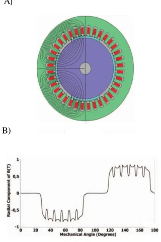
In (2.7) α is a coefficient found by Steinmetz and it can vary from 1.6 to 2.2. It depends on the level of the induction field that is mainly calculated in 1 or 1.5 T. While the coefficient Ki depends on the material, on the impurity and the geometrical structure of the stator. However, from the Fig. 2.14 it is clearly visible that each different point of the domain exhibits different value of the flux density due to the geometrical shape of the stator. Moreover, the produced magnetic field is far from a perfect sinusoidal waveform.

22

A)

B)

FIGURE 2.14: IN A) FLUX LINE MAP IN B) FLUX DENSITY DISTRIBUTION ALONG THE AIR GAP.

Therefore, the use of analytical formulas brings many assumptions that are often not true. Assuming the maximum value of the induced magnetic field for all the points of the stator is not correct and it may bring to errors [8]. Mainly for this reason, for the calculation of all the different iron losses a FEM analysis at least 2D is required.

Regarding the second term of (2.6), to avoid classical eddy-currents it is well known that the iron is laminated and any kind of electrical machine is assembled with many thick layers of iron, insulated between each other (Fig. 2.15). Moreover, the market offers mainly alloy of Silicon-Iron or Silicon-Steel to decrease the conductivity of Iron. The percentage of Silicon cannot be over 5/6% to avoid losing mechanical strength.

Eddy currents are the natural consequence of Faraday’s Law (2.8).

When a variable magnetic field is applied, in the perpendicular direction an EMF is created. Eddy currents circulate in closed loop on parallel planes.

23

FIGURE 2.15: BENEFIT OF A LAMINATED CORE AGAINST EDDY CURRENTS.

∇×𝐸̅ = −

∂B

̅

∂t

A common expression for stator eddy currents is

𝑃

= 𝐾

𝑓

𝐵

This analytical expression requires coefficients that strongly depend on the material and on the geometry of the magnetic sheet. Even though these values can be derived from the data sheets the accuracy achievable with this approach is quite poor. Furthermore, in the data sheets losses density is present for each different shape and dimensions. To have an approximate but reasonable value of the losses they offer a faster approach.

To increase the accuracy FEM analysis are needed to consider the different value of the varying maximum magnetic field in the different part of the stator. Moreover, other information about the material, the geometry and the air gap field are required. With this approach the Bertotti’s equation is often used in the calculation.

𝑃

= 𝐾

𝑓𝐵

+

𝜎𝑑

12

𝑑𝐵

𝑑𝑡

+ 𝐾

𝑑𝐵

𝑑𝑡

The first term is for the hysteresis losses while the second is for the eddy currents losses. The last one is the excess eddy currents losses [7]. Another important consideration is that for permanent magnet motor the waveform of the air gap field is far from sinusoidal and so to enhance the accuracy a precise description of that is needed.

24

While the iron losses of the stator are a secular topic of electrical machine, the theme about magnet losses is quite new in comparison but it grew in importance with the diffusion of pm motors. For the thermal constraints of the magnets this topic was investigated by many authors in order to predict the amount of losses produced and to avoid reaching the demagnetization temperature of the latter [9], [10]. The main contribution to magnet and rotor losses are eddy currents, hysteresis losses are generally smaller.

The physic principle is similar to the stator eddy-currents. But concerning the magnets the particular reasons can be individuated in: the lack of uniformity of the stator and the presence of harmonic content in the air gap field. Since the stator has often an open slot design, the magnets encounter alternatively part of iron and part of air that have very different permeance. This geometry causes additional harmonic as explained in [11]. Moreover, nowadays the problem is more and more important due to the use of power converters that can provide a high harmonic content in the currents that produce the magnetic field. As mentioned this kind of losses becomes significant in the PMSM machine and so it cannot be neglected [9]. The eddy currents path on the magnet is shown in Fig. 2.16.

The magnet and rotor losses are due to the presence of different harmonic contents in the magnetomotive force. In [11] it is explained that there are 3 different sources of harmonic content for the air gap field. This consideration is important also for chapter 3 in which the design, and the quality of the torque, will be discussed:

• space harmonics: armature windings and permanent magnet • time harmonics: ripple of the current generated by the inverter • slot permeance harmonics: iron and air alternate in open slot design

When the rotor runs, the magnet faces alternatively short air gap length areas under the iron and long air gap length under the slot. This causes an air gap field with a strong harmonic content that induces eddy currents in the magnet. The common adoption of not over-lapping concentrated windings increases the space harmonics [13], open slot design is very popular also and so slot permeance harmonics are significant. Moreover, the broad use of power converters frequency arises the problem of time harmonics.

25

FIGURE 2.16: EDDY CURRENTS ON THE PM.

The analytical expression is very complicated and it can be found in [10] and [12]. The stator windings are considered as an equivalent current sheet and the linear current density. The issue is that the current density of the rotor needs the solution of the magnetic vector potential that is often too complicated.

In [12] the losses are summarized with:

𝑃 ∼ 𝑙_𝑠∑ ∫𝐽𝑒 2 𝜎𝑑𝑆 𝑗 (2.13)

Where Je is the current density of the eddy currents on the magnets. Others [11] derive the

expression of the current density from Maxwell equation after the FEM analysis for the varying air gap field source of the voltage that produces this current.

Often the indirect method is used to calculate total iron losses. With different expedients, it is possible to measure losses in peculiar working points in which they should be only joule losses and mechanical. Because they can be estimated with a good accuracy without many efforts iron losses can be derived as the difference between total losses measured and the sum of joule and mechanical losses. The limit is that the test on the benchmark takes time and the evolution is very slow for the high thermal constant of the motor.

26

2.2.3 Mechanical Losses

The mechanical losses can be divided in bearing losses and windage losses. Bearing losses depend on the type of bearing, its lubricant but also rotor speed and load. An analytical expression can be found in [14]:

𝑃_𝐵 = 0.5𝜔_𝑚𝐾_𝐵𝐹𝐷_𝐵 (2.14)

Where ωm is the speed of the rotor, kB is a constant loss for the type of bearing, DB is the

diameter and F is the force acting on it. This latter can be derived from the configuration. Losses on the bearing are mainly due to the friction losses and a part of independent load losses in the lubricant.

Windage losses instead occur when friction is created between a rotating part and air. Unlike frictional losses they increase non-linearly with the force applied. The following expression can be used to calculate them:

𝑃𝑤 = 0.0315𝜔𝑚3𝜋𝐾𝑐𝑡𝐾𝑟𝜌𝑎𝑖𝑟𝐷𝑟4𝑙𝑟

(2.15)

Where Dr and lr are the diameter and length of the rotor. Kr is a coefficient for the

roughness. Kct is the torque coefficient and it can be derived separately: the Reynolds number has to be calculated to tell which kind of motion is occurring. Equations are found in [14]: 𝑁𝑅𝑒 = 𝜌_𝑎𝑖𝑟𝜔_𝑚𝐷_𝑟𝑙_𝑎𝑔 2𝜇𝑣𝑖𝑠(𝑎𝑖𝑟) (2.16) 𝐾_𝑐𝑡 = 2(2𝑙𝑎𝑔/𝐷𝑟) 0.3 𝑁_𝑅𝑒0.6 (2.17)

27

2.3 Gearbox Losses

The losses of the gearbox are a complicated issue, moreover it was not deeply investigated during the academic period because the field of study of the author is mainly electrical. Nevertheless, it is a component almost always present in the mechatronic chain and in many different applications. More recent technologies as direct drive try to avoid the use of gearboxes but this kind of application has a limited diffusion. There are many different types of industrial gearbox but the advantages of the choice of the planetary ones are remarkable. They may achieve better torsional stiffness and lower backlash than any other. However, the model of the losses becomes even more difficult for the increased significance of the independent load losses [17].

For this reason, this issue was not investigated in its singular details as CFD analysis. In chapter 4 a way to derive the efficiency maps is reported. Despite the complexity and the other difficulties just mentioned, efficiency evaluation are needed also on the gearboxes. Thus, the first step is to understand which losses are present.

Without the support of Doctor Franco Concli I would not have been able to obtain the efficiency map and to understand how they are calculated. Luckily, he already deeply analyzed the problem by a theoretical point of view [16].

In Fig. 2.17 the structure of a planetary gearbox is shown; a two-phase fluid of lubricant and air is present inside the case. The lubricant is continuously moved by the motion of the planets, its temperature and viscosity change and the two phases may mix up creating foam. The losses of a planetary gearbox can be divided in load dependent and load independent as in Fig. 2.17. No load (or independent load) losses occur even without power transmission while load dependent losses happen in the contact between the transmitting components. Moreover, they can be linked also to the different part of the gearboxes: meshing (or gears), bearing, seals and auxiliaries. The no load losses of gears and bearing are the losses due to the lubricant. It is worth to notice that even though they are usually classified load independent, because they strongly depend on the temperature, and a change of the load may change them. Fig. 2.18 shows a classification of the main gearbox losses dividing them on their dependence on the load.

28

FIGURE 2.17: STRUCTURE OF A PLANETARY GEARBOX.

FIGURE 2.18: CLASSIFICATION OF GEARBOX LOSSES [15].

For each of these losses a model is needed. All the losses are the results of complicated phenomena but analytical formulas that can calculate the losses only with the data from geometry and boundary conditions exist. In the planetary gearbox [16] the no load gears losses include also the fluid dynamics ones. Due to the structure and to the presence of the planet carrier [17] these losses arise in importance. The independent load losses are treated in a different way and rely on CFD analysis. They are the sum of churning, squeezing and windage losses. Basically, they are linked to the losses due to fluid dynamics reason of the two-phases fluid oil and air that lubricate the contact between the gears.

29

2.3.1 Meshing Losses

Load dependent

These kinds of losses are mainly due to the friction between the gears, in fact during the power transmission the motion is affected by sliding and rolling of the gears. Thus, they are proportional to the amount of torque transmitted. The most common formula to calculate them is [15]

𝑃𝐿𝐺=𝐹𝑅𝑣𝑟𝑒𝑙 = 𝐹𝑁𝜇𝑚𝑣𝑔

(2.18)

Where FR is the friction force, FN is the normal force, μm is the friction coefficient

achievable from a formula in [16] (need to notice that is function of the dynamical viscosity of the lubricant) and finally Vg is the sliding velocity.

Independent load losses

Specifically, for this kind of gearbox the churning and windage losses acquire particular significance because of the translational motion of the planets and the presence of the planet carrier [17]. The CFD analysis use the geometry of each different combination of teeth and ratio and calculate the field of pressure and speed of the two-phases fluid. The motion of the oil is complicated by viscosity and density changing with the temperature, moreover the motion of the planetary forces the oil to move and to mix with air. The oil tends to occupy particular areas, and to mix with air in others, to be squeezed near the contact of the gears while it is changing its properties due the changing of the temperature.

Churning losses are linked with the motion of the two-phases fluid and the unavoidable churning between itself and the planet-carrier of the planets. Furthermore, the contribution is divided between the resistant torque (viscous) due to the field of speed (2.19) and the inertial one due to pressure (2.20). Once the CFD analysis has obtained the velocity and pressure field they can be postprocessed.

The used formulas are generally (2.19) and (2.20) for each finite volume of the mesh grid [16]:

30 𝑇𝐿𝐺0𝜏=∑ 𝜈𝜄𝜌𝑚𝑖𝑥𝜄 𝜕𝑈_𝑖 𝜕𝑥𝑖 𝐴𝑖𝑟𝑖 (2.19) 𝑇_{𝐿𝐺0𝑝=}∑ 𝑝_𝜄𝐴_𝑖𝑟_𝑖 (2.20)

Where ν is the viscosity, ρ the density, U is the velocity, A is the area of the i-th cell, r is the radial distance of the i-th cell from the axis and p is the pressure field. The procedure is extended in case of a major number of stages for high transmission ratio repeating the simulation with the intermediate input (torque and speed) occurring at the second stage.

2.3.2 Bearing losses

As for the gear losses, they can be divided in load dependent and no load. The load dependent losses are due to the sliding between elements of the bearings, e.g. rings and rolling elements.

Independent load losses instead depend on the lubricant and on the geometry. They can be calculated knowing the properties of the oil and its interaction during the sliding of the rings. Bearing manufacturers investigated deeply the issue and propose analytical coefficient to derive bearing losses. An example of estimation of bearing load dependent losses [18]:

𝑃_𝐿𝐵= 1,05 ×10−4 _{𝑀 𝑛 (2.21)}

Where M is the total frictional moment, n is the speed.

2.3.3 Seal Losses

Seal losses are not dependent on the load. They are basically due to the sliding between the shaft and the seals themselves. Several reliable estimation methods are present in literature. Here (2.22) expresses a common way to calculate seal losses.

𝑃𝑣𝐷=𝜆𝑑2

𝑛 1000

31

λ is a coefficient that depends on the geometry and it describes the operating condition and temperature. d is the diameter and n is the rotational speed [16]

Eventually, it is worthy to notice that all these kinds of losses depend strongly on the temperature. Therefore, the model works only if the temperature in which the gearbox is working is known.

The amount of losses changes the heat dissipated and therefore the temperature. It is clear then that an iterative procedure is needed in the model.

As known, the viscosity of the lubricant decreases with higher temperature so, the friction coefficients and the load independent losses as well tend to decrease with an increase of the temperature along with the decrease of the viscosity and density of the lubricant. In fact, total gearbox losses exhibit a decrease with the increase of the temperature. The iterative procedure can reach an equilibrium point between the heat power dissipated (proportional to the temperature) and the losses that decrease with the temperature [16].

32

References Chapter 2

[1] Mohan N., Undeland T., Robbins W. - Power Electronics (II edition), John Wiley&Sons Inc.

[2] J. Pou, D. Osorno, J. Zaragoza, S. Ceballos, and C. Jaen, “Power Losses Calculation Methodology to Evaluate Inverter Efficiency in Electrical Vehicles,” IEEE Trans. Power Electron., pp. 404–409, 2011.

[3] P. Sanjeev, “Analysis of Conduction and Switching losses in two level inverter for low power applications,” 2013 Annu. IEEE INDICON, 2013.

[4] L. Song, “Efficiency Map Calculation for Surface-mounted Permanent-magnet In-wheel Motor Based on Design Parameters and Control Strategy,” ITEC Asia-Pacific, no. 2, pp. 1–6, 2014.

[5] G. Almandoz, G. Ugalde, J. Poza, and A. J. Escalada, “to Finite Element Software for Design and Analysis of Electrical Machines,” INTECH, 2012.

[6] Zijian Li (2012). Politecnico di Torino, Doctoral Thesis. Fractional slot concentrated winding surface-mounted permanent magnet motor design and analysis for in-wheel application.

[7] W. Roshen, “Iron Loss Model for Permanent-Magnet Synchronous Motors,” IEEE Trans. Magn., vol. 43, no. 8, pp. 3428–3434, 2007.

[8] Wu, X., Zhang, C., Wang, Y., Gang, D., Zhu, W., & Pan, L. (n.d.). The

Electromagnetic Losses Analysis of Surface-mounted Brushless AC PM machine Driven by PWM.

[9] N. Zhao and W. Liu, “Loss Calculation and Thermal Analysis of Surface-Mounted PM Motor and Interior PM Motor,” IEEE Trans. Magn., vol. 51, no. 11, pp. 2–5, 2015.

[10] K. Atallah, D. Howe, P. H. Mellor, and D. A. Stone, “Rotor Loss in Permanent-Magnet Brushless AC Machines,” IEEE Trans. Ind. Appl., vol. 36, no. 6, pp. 1612– 1618, 2000.

[11] J. Alexandrova, H. Jussila, and J. Nerg, “Comparison Between Models for Eddy-Current Loss Calculations in Rotor Surface-Mounted Permanent Magnets,” XIX Int. Conf. Electr. Mach. 2010, Rome, 2010.

[12] S. Steentjes, S. Boehmer, and K. Hameyer, “Permanent Magnet Eddy-Current Losses in 2-D FEM Simulations of Electrical Machines,” IEEE Trans. Magn., vol. 51, no. 3, pp. 3–6, 2015.

[13] Dutta R., Chong L., Rahamn F, “Analysis and experimental verification of losses in a concentrated wound interior permanent magnet machine.” Progress In

Electromagnetics Research B, Vol. 48, 221–248, 2013. (2013), 48(November 2012), 221–248.

33

[14] D. K. Athanasopoulos, V. I. Kastros, and J. C. Kappatou, “Electromagnetic Analysis of a PMSM with Different Rotor Topologies,” IEEE, vol. 1, 2016.

[15] Hohn, B. Michaelis, K., Hinterstoißer, M. “Optimization of gearbox efficiency.” Gomabn (2009) Volume: 48, Issue: 4, Pages: 462-480

[16] F. Concli, “Thermal and efficiency characterization of a low-backlash planetary gearbox: An integrated numerical-analytical prediction model and its experimental validation”.

[17] Conli F. Gorla C. “Le perdite per sbattimento in un riduttore epicicloidale.” Organi di trasmissione, (January 2012).

34

Chapter 3

STATE OF ART of EFFICIENCY in SERVO

DRIVES

This chapter presents the state of art to reduce the losses described in chapter 2 during the design process and in the control. To design an interesting product for customers it is obvious that increasing the efficiency cannot be the only goal. Thus, the discussion does not deal only with the efficiency problem but it mentions also the most common strategies used to obtain the best performance of the components.

As explained in the introduction, the field of application chosen is the Servo control. Due to high dynamic demand of Servo application, very compact and stiff components are needed to fulfil the requirements of the load. The highest power density and a very low inertia are therefore needed in order to develop an attractive solution and to satisfy the requirements. An investigation on the state of art of components is hereby presented focusing on the improvements more popular in the industry. The investigation is interested in benefit provided to these aspects:

• efficiency • power density

• maximum performance (static and dynamic)

• quality of the transmission: both electrical and mechanical power. • reliability

Typically, engineers look at possible improvements from three different approaches: • materials

• structure, dimensions or topology • control

Materials are always the key point but often the attractive property does not meet with all the other properties needed as cost, a trustful and stable supply, workability and transportability. Science will never stop to present new materials that will improve efficiency of all the 3 components. In power electronics, more discussion will be presented. The power electronics are a quite new field of research in comparison with electrical machine or speed reducer therefore many innovations are continuously presented. For